A collective Hamiltonian for the rotation–vibration motion of nuclei is considered, in which the axial quadrupole and octupole degrees of freedom are coupled through the centrifugal interaction. The potential of the system depends on the two deformation variables $\beta_{2}$ and $\beta_{3}$. The system is considered to oscillate between positive and negative $\beta_{3}$-values, by rounding an infinite potential core in the $(\beta_{2},\beta_{3})$-plane with $\beta_{2}>0$. By assuming a coherent contribution of the quadrupole and octupole oscillation modes in the collective motion, the energy spectrum is derived in an explicit analytic form, providing specific parity shift effects. On this basis several possible ways in the evolution of quadrupole–octupole collectivity are outlined. A particular application of the model to the energy levels and electric transition probabilities in alternating parity spectra of the nuclei ¹⁵⁰Nd, ¹⁵²Sm, ¹⁵⁴Gd and ¹⁵⁶Dy is presented.

PACS: 21.60.Ev; 21.10.Re

1 Introduction

Shape deformations and surface oscillations in atomic nuclei determine from a geometric point of view the main features of nuclear collective dynamics [1]. The leading quadrupole mode manifests itself in all regions of collectivity providing vibrational, rotational, and transitional structures of the spectra. In addition, in some regions the manifestation of octupole degrees of freedom is superposed, leading to more complicated shape properties and parity effects in the spectrum of the system [2, 3]. A variety of microscopic, geometric and algebraic model approaches have been applied in nuclear regions where the quadrupole and octupole degrees of freedom coexist [3].

In general, the problem of quadrupole–octupole collectivity is not easy to solve neither microscopically, mainly due to the breaking of reflection symmetry, nor geometrically, due to the difficulty in determining the total inertia tensor of the system. It is, however, simplified considerably if the axial symmetry is still preserved and if the octupole deformations are fixed appropriately with respect to the principal axes of the quadrupole shape. Further simplification is achieved if both degrees of freedom are separated adiabatically. It allows one to examine the manifestation of the octupole mode for fixed values of quadrupole parameters. In such a case the collective motion can be associated to the oscillations of the reflection asymmetric shape with respect to an octupole variable $\beta_{3}$ in a double-well potential [4, 5]. Then the parity shift effect observed in nuclear alternating parity bands can be explained as the result of the tunnelling through the potential barrier [6, 7]. This concept has been generalized for the case of simultaneously contributing quadrupole and octupole modes [8], as well as for the case of higher multipole degrees of freedom [9]. In both cases the double-well potential was defined in terms of a variable carrying the relative contribution of the different degrees of freedom and not the absolute values of the respective deformation variables. In such a way the explicit form of the original potential in terms of the quadrupole $\beta_{2}$ and octupole $\beta_{3}$ deformation variables was not given. As a consequence, some basic characteristics of the quadrupole and octupole modes and their interaction remain outside of consideration. Such is the behavior of the system in dependence on the quadrupole and octupole stiffness, as well as the limiting case of a frozen quadrupole variable. Another interesting question is, if and to what extent one may consider the presence of a tunnelling effect in the space of the octupole variable $\beta_{3}$ after the quadrupole coordinate $\beta_{2}$ is let to vary. Some limiting cases in the shape evolution and the angular momentum properties of the system are also of interest in respect with the above.

The purpose of the present work is to clarify the above questions by applying a simple explicit form of the collective energy potential as a function of the quadrupole and octupole axial deformation variables $\beta_{2}$ and $\beta_{3}$. We examine the evolution of the potential shape in dependence on both degrees of freedom, as well as on the collective angular momentum. The geometric analysis suggests that the oscillations of the system in the two-dimensional case of simultaneous manifestation of the quadrupole and octupole modes are performed in a different way, compared to the one-dimensional case of a reflection asymmetric shape with a frozen quadrupole variable. We study the physical consequences of the two-dimensional oscillations and demonstrate their role in the rotation-vibration motion of the system.

In particular, the explicit geometric analysis of the quadrupole–octupole potential suggests a possibility for a coherent interplay between both collective modes. This allows the derivation of explicit analytic expressions for the energy levels and electromagnetic transition probabilities applicable to nuclei in which an “equal” (coherent) manifestation of quadrupole and octupole degrees of freedom is considered. As a result, one is able to study in detail the respective effects in the structure of the spectrum. Below it will be shown that such a consideration can be applied reasonably to some nuclei in the rare earth region, such as the $N=90$ isotones ¹⁵⁰Nd, ¹⁵²Sm, ¹⁵⁴Gd and ¹⁵⁶Dy. These nuclei are also a subject of interest [10, 11] from the point of view of the X(5) critical point symmetry [12] between quadrupole vibrations [U(5)] and axial quadrupole deformation [SU(3)]. In the present work we shall, however, mainly consider the common quadrupole-octupole collective properties, which, in principle, can take place in various nuclear regions.

In Sec. 2 the Hamiltonian of the coupled quadrupole and octupole modes is presented, together with the geometric analysis of the quadrupole–octupole potential. In Sec. 3 the Schrödinger equation is considered in the case of a coherent interplay between the two degrees of freedom. The analytic solutions for several particular forms of the potential and the respective schematic spectra are given in Sec. 4. In addition, results of the model description of alternating parity spectra in ¹⁵⁰Nd, ¹⁵²Sm, ¹⁵⁴Gd and ¹⁵⁶Dy are presented. The electric transition probabilities are considered in Sec. 5, while in Sec. 6 a brief discusssion of the influence of the $\gamma$ degree of freedom on the present results is given. Finally, a summary and concluding remarks are given in Sec. 7.

2 Hamiltonian for the coupled quadrupole and octupole modes

We assume that the system is allowed to oscillate with respect to the quadrupole $\beta_{2}$ and octupole $\beta_{3}$ axial deformation variables. In addition, both degrees of freedom are coupled through a centrifugal (rotation-vibration) interaction depending on the collective angular momentum $I$. The energy potential represents a two-dimensional surface determined by the variables $\beta_{2}$ and $\beta_{3}$.

The quadrupole–octupole Hamiltonian describing the collective motion under the above assumptions has the form

$$H_{qo} = -\frac{\hbar^{2}}{2B_{2}}\frac{\partial^{2}}{\partial\beta_{2}^{2}}-\frac{\hbar^{2}}{2B_{3}}\frac{\partial^{2}}{\partial\beta_{3}^{2}}+U(\beta_{2},\beta_{3},I)\ ,$$ (1)

where the potential is

$$U(\beta_{2},\beta_{3},I)=\frac{1}{2}C_{2}{\beta_{2}}^{2}+\frac{1}{2}C_{3}{\beta_{3}}^{2}+\frac{X(I)}{d_{2}\beta_{2}^{2}+d_{3}\beta_{3}^{2}},$$ (2)

with $X(I)=I(I+1)/2$. Here $B_{2}$ and $B_{3}$ are the effective quadrupole and octupole mass parameters, and $C_{2}$ and $C_{3}$ are the stiffness parameters for the respective oscillation modes.

The last term in Eq. (2) provides a coupling between quadrupole and octupole degrees of freedom. Its denominator can be associated to the moment of inertia of an axially symmetric quadrupole-octupole deformed shape, ${\mathcal{J}}^{(quad+oct)}=3B_{2}\beta_{2}^{2}+6B_{3}\beta_{3}^{2}$ [13]. Therefore, the constants $d_{2},\,d_{3}>0$ can be related to the mass parameters as $d_{2}=3B_{2}$ and $d_{3}=6B_{3}$. However, in the present study we do not impose this relation and below a more general correlation between $d_{2},\,B_{2}$ and $d_{3},\,B_{3}$ is considered. The quantities $d_{2}$ and $d_{3}$ determine the contributions of the quadrupole and octupole modes, respectively, to the moment of inertia. Also, we remark that if the ground state of the system is considered ($I=0$), the potential $U(\beta_{2},\beta_{3},I)$ should be taken by replacing $X(I)\rightarrow d_{0}+X(I)$, with $d_{0}$ being a constant.

The Hamiltonian (1) represents a two-dimensional generalization of the soft octupole oscillator Hamiltonian introduced in [14], as well as of the one-dimensional octupole Hamiltonian derived in [15]. In the latter two approaches the quadrupole mode is assumed frozen as mentioned in Sec. 1. In this respect, Eq. (1) corresponds to an extension in which the quadrupole coordinate is let to vary. Also, it corresponds to the quadrupole–octupole Hamiltonian in Refs. [8, 9]. However, in the present work the potential energy (2) is taken in an explicit form depending on $\beta_{2}$ and $\beta_{3}$ (including the harmonic oscillator part), while in Refs. [8, 9] a double-oscillator potential is defined in the space of polar coordinates. In this way, the explicit form of Eq. (2) allows one to examine in detail the potential surface and its dependence on the model parameters and the collective angular momentum.

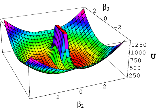
Figure 1: (Color online) Schematic 3D plot of the potential $U(\beta_{2},\beta_{3},I)$, Eq. (2), in MeV for $I=5$ as a function of $\beta_{2}$ and $\beta_{3}$. The parameter values are $C_{2}=C_{3}=100$ MeV, $d_{2}=0.1$ $\hbar^{2}$MeV^-1, and $d_{3}=0.01$ $\hbar^{2}$MeV^-1.

Figure 2: Schematic numerical behavior of the potential $U(\beta_{2},\beta_{3},I)$, Eq. (2), in MeV for $I=1$ as a function of: (a) $\beta_{2}$ at fixed $\beta_{3}=0.1$; (b) $\beta_{3}$ at fixed $\beta_{2}=0.25$. The parameter values are $C_{2}=C_{3}=100$ MeV, $d_{2}=0.1$ $\hbar^{2}$MeV^-1, and $d_{3}=0.01$ $\hbar^{2}$MeV^-1.

Having in mind that the quadrupole deformation has the leading role in the rotation mode, we assume that its contribution to the moment of inertia is larger than the octupole contribution. This assumption corresponds to the condition $d_{2}>d_{3}$, e.g. we can take $d_{2}=0.1$ $\hbar^{2}$MeV^-1 and $d_{3}=0.01$ $\hbar^{2}$MeV^-1. Then, for comparable values of the deformation variables $\beta_{2}$ and $\beta_{3}$, the input of the quadrupole mode in the denominator of the centrifugal term will be larger than the octupole one. On the other hand, as it will be seen in Sec. 3, this circumstance does not restrict the possibility of equal (coherent) contributions of both degrees of freedom in the mixed quadrupole–octupole oscillation mode. Moreover, since the rotation and vibration modes are coupled, the above condition might be not strictly imposed. In this meaning the considered values of $d_{2}$ and $d_{3}$ provide only a schematic geometric analysis of the potential (2).

Let us now examine the minimum of the potential energy in dependence on the model parameters. The set of extremum conditions for the coordinates of the two-dimensional minimum ($\beta_{2min},\beta_{3min}$) is

$$\left.\frac{\partial}{\partial\beta_{2}}U(\beta_{2},\beta_{3},I)\right|_{(\beta_{2min},\beta_{3min})}=0\ \ \mbox{and}\ \ \left.\frac{\partial}{\partial\beta_{3}}U(\beta_{2},\beta_{3},I)\right|_{(\beta_{2min},\beta_{3min})}=0;$$ (3)

$$\left.\frac{\partial^{2}}{\partial\beta_{2}^{2}}U(\beta_{2},\beta_{3},I)\right|_{(\beta_{2min},\beta_{3min})}>0\ \ \mbox{and}\ \ \left.\frac{\partial^{2}}{\partial\beta_{3}^{2}}U(\beta_{2},\beta_{3},I)\right|_{(\beta_{2min},\beta_{3min})}>0.$$ (4)

It determines the following possible cases for the bottom of the potential,

i) $\beta_{3min}=0$; $\beta_{2min}=\pm\left[2X(I)/(d_{2}C_{2})\right]^{1/4}$;

ii) $\beta_{2min}=0$; $\beta_{3min}=\pm\left[2X(I)/(d_{3}C_{3})\right]^{1/4}$;

iii) $\beta_{2min}\neq 0$ and $\beta_{3min}\neq 0$ with the condition

$$C_{2}=\frac{2X(I)d_{2}}{(d_{2}\beta_{2min}^{2}+d_{3}\beta_{3min}^{2})^{2}}\ \ \mbox{and}\ \ C_{3}=\frac{2X(I)d_{3}}{(d_{2}\beta_{2min}^{2}+d_{3}\beta_{3min}^{2})^{2}}\ .$$ (5)

The shape of the potential corresponding to the case i) is illustrated in Fig. 1. It is characterized by two energy minima for $\beta_{2}>0$ and $\beta_{2}<0$ separated by a well determined potential barrier. For given sign of $\beta_{2}$ (we consider $\beta_{2}>0$) the bottom of the potential is not separated in the $\beta_{3}$- direction, allowing oscillations of the system between $\beta_{3}>0$ and $\beta_{3}<0$. This situation is illustrated in Fig. 2. We see that for a fixed physically typical value of $\beta_{3}$ (Fig.2a) the barrier in the quadrupole space of $\beta_{2}$ is very large. Thus it restricts the values of the quadrupole deformation within the half space $\beta_{2}>0$. For a fixed typical $\beta_{2}$- value (Fig.2b) the barrier in the octupole space of $\beta_{3}$ is relatively small. From Fig. 1 it is seen that for some higher $\beta_{2}$- values this barrier is reduced, and for $\beta_{2}\geq\beta_{2min}$ it disappears ($\beta_{3min}=0$).

In the case ii) the potential shape is the same as in Fig. 1, but the coordinates $\beta_{2}$ and $\beta_{3}$ are exchanged. As far as the system is not considered to oscillate between positive and negative $\beta_{2}$ deformations, this case is not of interest in the context of the present analysis.

Figure 3: (Color online) Schematic 3D plot of the potential $U(\beta_{2},\beta_{3},I)$, Eq. (2), in MeV for $I=5$ as a function of $\beta_{2}$ and $\beta_{3}$. The parameter values are $C_{2}=100$ MeV, $C_{3}=10$ MeV $d_{2}=0.1$ $\hbar^{2}$MeV^-1, and $d_{3}=0.01$ $\hbar^{2}$MeV^-1.

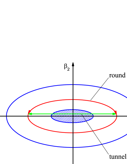
Figure 4: (Color online) Schematic picture of the tunnelling and the rounding way in the $\beta_{3}$- variable. See Sec. 2 for further discussion.

In the case iii) of non-zero $\beta_{2min}$ and $\beta_{3min}$, Eq. (5) imposes the relation

$$\frac{d_{2}}{C_{2}}=\frac{d_{3}}{C_{3}}\ .$$ (6)

It determines an elliptic form of the bottom of the two-dimensional potential surface given by $\beta_{2min}^{2}/\sqrt{2X(I)/(d_{2}C_{2})}+\beta_{3min}^{2}/\sqrt{2X(I)/(d_{3}C_{3})}=1$. The shape of the potential corresponding to the case iii) is illustrated in Fig. 3. It suggests that the system moves in the two-dimensional space of the deformation variables $\beta_{2}$ and $\beta_{3}$ by rounding the internal potential core. If a prolate quadrupole deformation is considered, the rounding is performed between positive and negative $\beta_{3}$ values in the space of $\beta_{2}>0$. This situation can be considered as the two-dimensional extension of the one-dimensional case in which the $\beta_{2}$ coordinate is frozen. To explain this in detail, we consider a horizontal (equipotential) intersection of the shape in Fig. 3, which is illustrated schematically in Fig. 4. We see that if the quadrupole coordinate is fixed at some value of $\beta_{2}>0$, the motion in the octupole coordinate between positive and negative $\beta_{3}$-values is characterized by the tunnelling through a potential barrier (a vertical intersection of the core). When $\beta_{2}$ is let to vary, the tunnelling is replaced by a motion along the curved way rounding the potential core.

The above case iii) is of particular interest, due to the simultaneous presence of non-zero coordinates of the potential minimum in both degrees of freedom. It suggests that the oscillations in the quadrupole and octupole coordinates are involved in the collective motion on the same footing. As it will be seen below, such a situation appears to take place in certain nuclear regions. Moreover, it will be seen that the ellipsoidal symmetry in the potential bottom allows, under some additional conditions, a complete analytic determination of the energy spectrum. This is why in the following we shall imply this case, unless something different is indicated. Also, we assume only the presence of prolate quadrupole deformations. This is why hereafter we consider only the $\beta_{2}>0$ part of the space.

Further, we examine the evolution of the potential shape with the angular momentum $I$. We consider the following two cases.

I) The potential minimum (the 2-dimensional bottom) is allowed to change with $I$ for fixed values of the stiffness parameters $C_{2}$ and $C_{3}$.

II) The minimum is fixed, so that the values $\beta_{2min}$ and $\beta_{3min}$ determine an ellipse which does not change with the angular momentum.

It is clear that in the case I) of fixed stiffness parameters, the quadrupole and the octupole deformations corresponding to the potential minimum should exhibit an overall increase in the denominator of Eqs. (5) with increasing $I$.

In the case II) of fixed minima, the stiffness parameters $C_{2}\equiv C_{2}(I)$ and $C_{3}\equiv C_{3}(I)$ increase quadratically with $I$ according to the right hand sides of (5). Then the substitution of Eqs. (5) into (2), leads to the following form of the quadrupole–octupole potential

$$U(\beta_{2},\beta_{3},I) = X(I)\left(\frac{d_{2}\beta_{2}^{2}+d_{3}\beta_{3}^{2}}{(d_{2}\beta_{2min}^{2}+d_{3}\beta_{3min}^{2})^{2}}+\frac{1}{d_{2}\beta_{2}^{2}+d_{3}\beta_{3}^{2}}\right)\ .$$ (7)

If the origin of the energy scale is fixed at the potential minimum, one has

$$U_{I}(\beta_{2},\beta_{3}) = U(\beta_{2},\beta_{3},I)-U(\beta_{2min},\beta_{3min},I)$$ (8)

$$= \frac{X(I)[d_{2}(\beta_{2}^{2}-\beta_{2min}^{2})+d_{3}(\beta_{3}^{2}-\beta_{3min}^{2})]^{2}}{(d_{2}\beta_{2min}^{2}+d_{3}\beta_{3min}^{2})^{2}(d_{2}\beta_{2}^{2}+d_{3}\beta_{3}^{2})}.$$

We remark that the potential (7) includes the rotational contribution of the centrifugal term, which moves up the energy with increasing angular momentum $I$. On the other hand, in the potential (8) the explicit contribution of the rotational degree of freedom is diminished, so that the energy term keeps mainly the vibrational component. The shape of the potential (8) with $\beta_{2}>0$ is illustrated in Fig. 5.

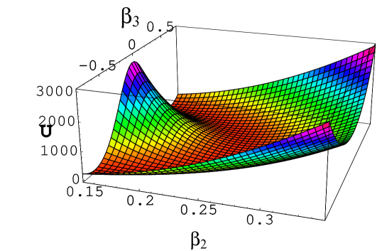
Figure 5: (Color online) 3D plot of the potential $U_{I}(\beta_{2},\beta_{3})$, Eq. (8), in MeV for $I=5$ as a function of $\beta_{2}$ and $\beta_{3}$ with $\beta_{2min}=0.25$, $\beta_{3min}=0.1$, $d_{2}=0.1$ $\hbar^{2}$MeV^-1, and $d_{3}=0.01$ $\hbar^{2}$MeV^-1.

3 Model potentials and the Schrödinger equation in polar variables

Further, it is convenient to introduce polar variables $\eta$ and $\phi$ by taking

$$\beta_{2}=\frac{\eta}{\sqrt{d_{2}/d}}\cos\phi\ ;\qquad\beta_{3}=\frac{\eta}{\sqrt{d_{3}/d}}\sin\phi\ ,$$ (9)

with $d=(d_{2}+d_{3})/2$. Considering $\beta_{2}>0$, we have

$$\eta=\frac{1}{\sqrt{d}}\sqrt{d_{2}\beta_{2}^{2}+d_{3}\beta_{3}^{2}}\ ;\qquad\phi=\arctan\left({\frac{\beta_{3}}{\beta_{2}}\sqrt{\frac{d_{3}}{d_{2}}}}\right)\ ,$$ (10)

where the “effective” deformation variable $\eta$ is defined with positive values $\eta>0$, while the relative (“angular”) variable $\phi$ is defined in the interval $-\pi/2\leq\phi\leq\pi/2$. We remark that the negative $\phi$- values correspond to negative $\beta_{3}$. (The variable $\beta_{3}$ takes both positive and negative values.)

Then the quadrupole-octupole Hamiltonian (1) can be written in the form

$$H_{qo} = -\frac{\hbar^{2}\,d_{2}}{2dB_{2}}\left[\cos^{2}{\phi}\frac{\partial^{2}}{\partial\eta^{2}}+\frac{1}{\eta}\sin^{2}{\phi}\frac{\partial}{\partial\eta}+\frac{1}{\eta^{2}}\sin^{2}{\phi}\frac{\partial^{2}}{\partial\phi^{2}}\right.$$ (11)

$$+ \left.2\frac{1}{\eta^{2}}\sin{\phi}\,cos{\phi}\frac{\partial}{\partial\phi}-2\frac{1}{\eta}\sin{\phi}\,cos{\phi}\frac{\partial^{2}}{\partial\eta\partial\phi}\right]$$

$$- \frac{\hbar^{2}\,d_{3}}{2dB_{3}}\left[\sin^{2}{\phi}\frac{\partial^{2}}{\partial\eta^{2}}+\frac{1}{\eta}\cos^{2}{\phi}\frac{\partial}{\partial\eta}+\frac{1}{\eta^{2}}\cos^{2}{\phi}\frac{\partial^{2}}{\partial\phi^{2}}\right.$$

$$- \left.2\frac{1}{\eta^{2}}\sin{\phi}\,cos{\phi}\frac{\partial}{\partial\phi}+2\frac{1}{\eta}\sin{\phi}\,cos{\phi}\frac{\partial^{2}}{\partial\eta\partial\phi}\right]+$$

$$+ U_{I}(\eta)\ .$$

Under the condition (6), the potential energy depends only on the effective deformation variable $\eta$ and on the angular momentum $I$, and not on the relative (angular) variable $\phi$. Then in the case I) of fixed stiffness parameters one has

$$U_{I}(\eta)=\frac{1}{2}C\eta^{2}+\frac{X(I)}{d\eta^{2}}\ \qquad\qquad(\mathrm{Case\ I}),$$ (12)

where $C$ is defined according to Eq. (6) as $1/C=d_{2}/(dC_{2})=d_{3}/dC_{3}$.

In the case II) of fixed minima the potential term appears in the following two forms

$$U_{I}(\eta) = X(I)\frac{\eta^{4}+\eta_{min}^{4}}{d\eta_{min}^{4}\,\eta^{2}}\ \ \ \qquad\qquad(\mathrm{Case\ II.A});$$ (13)

$$U_{I}(\eta) = X(I)\frac{[\eta^{2}-\eta_{min}^{2}]^{2}}{d\eta_{min}^{4}\,\eta^{2}}\qquad\qquad(\mathrm{Case\ II.B}),$$ (14)

where Eq. (13) corresponds to the rotation dependent potential (7), while Eq. (14) represents the essentially vibrational term (8). The quantity $\eta_{min}=(1/\sqrt{d})(d_{2}\beta_{2min}^{2}+d_{3}\beta_{3min}^{2})^{1/2}$ is the value of the variable $\eta$ in the potential minimum. In the following we shall refer to Eq. (13) as case II.A and to Eq. (14) as case II.B.

Using the effective deformation variable $\eta$ we are also capable to examine a third case (III) of an infinite square well with an infinite core at zero defined as

$$U^{I}_{\mathrm{w}}(\eta) = \left\{\begin{array}[]{cc}\frac{X(I)}{d\eta^{2}}&\eta\leq\eta_{\mathrm{w}}\\ \infty&\ \ \eta>\eta_{\mathrm{w}}\end{array}\right.\qquad\qquad(\mathrm{Case\ III}),$$ (17)

where $\eta_{\mathrm{w}}$ is a parameter determining the width of the well.

Now we assume the following relation between the quadrupole and octupole mass and inertia parameters

$$\frac{d_{2}}{dB_{2}}=\frac{d_{3}}{dB_{3}}=\frac{1}{B}\ .$$ (18)

This leads to the following form of the model Hamiltonian

$$H_{qo} = -\frac{\hbar^{2}}{2B}\left[\frac{\partial^{2}}{\partial\eta^{2}}+\frac{1}{\eta}\frac{\partial}{\partial\eta}+\frac{1}{\eta^{2}}\frac{\partial^{2}}{\partial\phi^{2}}\right]+U_{I}(\eta)\ .$$ (19)

The assumption (18), which much simplifies the problem, suggests that $d_{2}$ and $d_{3}$ are related to the mass parameters $B_{2}$ and $B_{3}$ respectively, through the same coefficient $d/B$. By comparing Eq. (18) and Eq. (6), we obtain $C_{2}/B_{2}=C_{3}/B_{3}$, or $\omega_{2}^{2}=\omega_{3}^{2}$, i.e. the assumption (18) implies that both degrees of freedom, quadrupole and octupole, are characterized by equal angular frequencies $\omega_{2}$ and $\omega_{3}$, respectively. This means that a coherent interplay between the two collective modes is assumed. In other words, the condition (18) suggests that the oscillations in the quadrupole and octupole coordinates are represented in the collective motion on the same footing. The quantity $B$ in Eq. (18) has the meaning of the effective mass of the total quadrupole–octupole system.

The Schrödinger equation for the Hamiltonian (19) has the form

$$-\frac{\hbar^{2}}{2B}\frac{1}{\eta^{2}}\left[\frac{\eta^{2}\partial^{2}}{\partial\eta^{2}}+\eta\frac{\partial}{\partial\eta}+\frac{\partial^{2}}{\partial\phi^{2}}\right]\Phi(\eta,\phi)+U_{I}(\eta)\Phi(\eta,\phi)=E\Phi(\eta,\phi)\ .$$ (20)

After dividing it by $\hbar^{2}/(2B\eta^{2})$ and separating the variables $\eta$ and $\phi$ through $\Phi(\eta,\phi)=\psi(\eta)\varphi(\phi)$ we obtain the following two equations

$$\frac{\partial^{2}}{\partial\eta^{2}}\psi(\eta)+\frac{1}{\eta}\frac{\partial}{\partial\eta}\psi(\eta)+\frac{2B}{\hbar^{2}}\left[E-\frac{\hbar^{2}}{2B}\frac{k^{2}}{\eta^{2}}-U_{I}(\eta)\right]\psi(\eta) = 0\ ;$$ (21)

$$\frac{\partial^{2}}{\partial\phi^{2}}\varphi(\phi)+k^{2}\varphi(\phi) = 0\ ,$$ (22)

where $k$ is the separation quantum number.

4 Analytic solutions and numerical results

In the following we give analytic solutions of the above equations in the cases I-III with the potentials (12), (13), (14), and (17).

In the Case I, after introducing the potential (12) into Eq. (21) we have

$$\frac{\partial^{2}}{\partial\eta^{2}}\psi(\eta)+\frac{1}{\eta}\frac{\partial}{\partial\eta}\psi(\eta)+\frac{2B}{\hbar^{2}}\left[E-\frac{\hbar^{2}}{2B}\frac{k^{2}}{\eta^{2}}-\frac{1}{2}C\eta^{2}-\frac{X(I)}{d\eta^{2}}\right]\psi(\eta)=0\ .$$ (23)

By introducing a reduced energy $\varepsilon=\frac{2B}{\hbar^{2}}E$ and a reduced angular momentum factor $\widetilde{X}(I)=bX(I)$, with $b=\frac{2B}{\hbar^{2}d}$, we obtain Eq. (23) in the form

$$\frac{\partial^{2}}{\partial\eta^{2}}\psi(\eta)+\frac{1}{\eta}\frac{\partial}{\partial\eta}\psi(\eta)+\left[\varepsilon-\frac{k^{2}+\widetilde{X}(I)}{\eta^{2}}-\frac{BC}{\hbar^{2}}\eta^{2}\right]\psi(\eta)=0\ .$$ (24)

The effective potential appearing in the brackets of Eq. (24) is of a form similar to the Davidson potential [16], which is analytically solvable [17, 18]. Thus Eq. (24) can be solved analytically and we obtain the following explicit expression for the energy spectrum

$$E_{n,k}(I)=\hbar\omega\left[2n+1+\sqrt{k^{2}+\widetilde{X}(I)}\right],$$ (25)

where $\omega=\sqrt{C/B}$ and $n=0,1,2,...$. The eigenfunctions $\psi(\eta)$ of Eq. (23) are obtained in terms of the Laguerre polynomials

$$\psi^{I}_{n}(\eta)=\sqrt{\frac{2\Gamma(n+1)}{\Gamma(n+2s+1)}}e^{-a\eta^{2}/2}a^{s}\eta^{2s}L^{2s}_{n}(a\eta^{2})\ ,$$ (26)

where $a=\sqrt{BC}/\hbar$ and $s=\sqrt{k^{2}+\widetilde{X}(I)}/2$.

Now we remark that Eq. (22) in the variable $\phi$ is solved under the periodic boundary condition $\varphi(\phi+2\pi)=\varphi(\phi)$. On the other hand the assumption $\beta_{2}>0$, which is equivalent to the consideration of an infinite potential wall at $\beta_{2}=0$ (or $\phi=\pm\pi/2$), imposes the additional condition

$$\varphi(-\pi/2)=\varphi(\pi/2)=0\ .$$ (27)

Eq. (22) has two different solutions satisfying the condition (27) with positive, $\pi=(+)$, and negative, $\pi=(-)$, parity as follows

$$\varphi^{+}(\phi) = \sqrt{2/\pi}\cos(k\phi)\ ,\qquad k=\pm 1,\pm 3,\pm 5,...\ ;$$ (28)

$$\varphi^{-}(\phi) = \sqrt{2/\pi}\sin(k\phi)\ ,\qquad k=\pm 2,\pm 4,\pm 6,...\ .$$ (29)

Eq. (28) provides positive parity for the intrinsic wave function, while Eq. (29) corresponds to a negative parity function. As a result, the intrinsic wave function appears in the form $\Phi^{\pm}(\eta,\phi)=\psi(\eta)\varphi^{\pm}(\phi)$. On the other hand, the $\mathcal{R}\mathcal{P}$- symmetry of the total wave function of the system, $\Psi\sim\Phi^{\pm}(\eta,\phi)|IKM\rangle$, has to be conserved. The $\mathcal{R}$- symmetry of the rotation function $|IKM\rangle$ is characterized by the factor $(-1)^{I}$. For the total state of the system one has $\pi(-1)^{I}=1$. It follows that for $I$=even the quantum number $k$ is allowed to take the values $k_{(+)}=1,3,5,\dots$, corresponding to the even function (28), while for $I$=odd one has $k_{(-)}=2,4,6,\dots$ corresponding to the odd function (29). Thus, when the angular momentum is changed from $I$=odd to $I$=even and vice versa, the respective values of the quantum number $k$ should switch between $k_{(-)}$ and $k_{(+)}$. This parity effect provides an odd-even staggering structure of the spectrum (25). We consider that the lowest states of the system with respect to the variable $\phi$ are characterized by the lowest $k$- values, $k_{(+)}=1$ for $I=$even and $k_{(-)}=2$ for $I=$odd. Therefore, the staggering behavior of the model spectrum is provided by the difference $\Delta k^{2}=k_{(-)}^{2}-k_{(+)}^{2}=3$.

  

Figure 6: Schematic energy levels (a) and staggering pattern (b) for the spectrum (25) with $n=0$. The parameter values are shown in part (a), $\omega$ is given in MeV$/\hbar$, while $b$ and $d_{0}$ are in $\hbar^{-2}$ and $\hbar^{2}$ respectively.

In such a way the energy expression (25), with the parity-dependent quantum number $k$, determines the structure of an alternating parity spectrum. The energy levels $E_{0,k}(I)$, with $n=0$, correspond to the yrast alternating parity sequence. The levels with $n\neq 0$ correspond to higher energy bands, in which the rotational states are built on quadrupole–octupole (mixed $\beta_{2}$-$\beta_{3}$) vibrations of the system. In this case, the states with even $I$ appear similarly to the states of a higher $\beta$- (quadrupole) band. Thus, the present model suggests that, in the nuclear regions with quadrupole–octupole collectivity, one may consider “octupole mixed” $\beta$- band structures. We remark that, in the present model framework, the $\gamma$- bands are not included. This can be done in an extended formalism allowing the simultaneous consideration of the $\gamma$- variable. In addition, the octupole triaxiality can be taken into account. Then one may also discuss possible “octupole admixtures” in the $\gamma$- band structure.

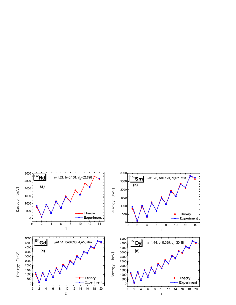
Figure 7: (Color online) Theoretical and experimental energy levels for the alternating parity bands in ¹⁵⁰Nd (data from [19]), ¹⁵²Sm (data from [20]), ¹⁵⁴Gd (data from [21]) and ¹⁵⁶Dy (data from [22]). The theoretical results are obtained by (25) with $n=0$. The parameter units are as in Fig. 6.

Figure 8: (Color online) Theoretical and experimental staggering patterns for the alternating parity bands in ¹⁵⁰Nd, ¹⁵²Sm, ¹⁵⁴Gd and ¹⁵⁶Dy. The theoretical results are obtained by (25) with $n=0$. The parameter units are as in Fig. 6.

We can estimate analytically the staggering effect at higher angular momenta, where $\Delta k^{2}\ll\widetilde{X}(I)$. The square root term $\sqrt{k^{2}+\widetilde{X}(I)}$ in Eq. (25) can be expanded as $\sqrt{\widetilde{X}(I)}+k^{2}/(2\sqrt{\widetilde{X}(I)})$. We see that the term $k^{2}/(2\sqrt{\widetilde{X}(I)})$, which is responsible for the staggering effect, decreases nearly linearly with the angular momentum $I$ since $\widetilde{X}(I)=bX(I)\sim I(I+1)$. We consider the quantity $b=2B/(\hbar^{2}d)$ as a model parameter. The numerical behavior of the energy and the staggering effect for the spectrum (25) is illustrated in Fig. 6. The staggering effect is illustrated in terms of the five point quantity

$$\mbox{Stg}(I)=6\Delta E(I)-4\Delta E(I-1)-4\Delta E(I+1)+\Delta E(I+2)+\Delta E(I-2)\ ,$$ (30)

where $\Delta E(I)=E(I+1)-E(I)$. The schematic staggering pattern suggests that the odd and even angular momentum sequences approach each other towards higher angular momenta. It outlines a trend for the forming of an octupole band. However, the linear decrement of the staggering amplitude is not enough to provide such a band structure at reasonable (experimentally observed) angular momenta. A similar situation is observed in rare earth nuclei, where the alternating parity levels approach each other without merging into a single band.

On this basis, we applied Eq. (25) to describe the alternating parity spectra in the nuclei ¹⁵⁰Nd, ¹⁵²Sm, ¹⁵⁴Gd, and ¹⁵⁶Dy. The theoretical energies are obtained by taking $\widetilde{E}_{n,k}(I)=E_{n,k}(I)-E_{n,k}(0)$, with $n=0$ and $X(I)=\frac{1}{2}[d_{0}+I(I+1)]$, where the parameter $d_{0}$ characterizes the potential shape in the ground state, as mentioned in the paragraph after Eq. (2). The parameters $\omega$, $b$ and $d_{0}$ are adjusted to the energy levels by means of a least square minimization procedure.

In Fig. 7 results for the energy levels of ¹⁵⁰Nd, ¹⁵²Sm, ¹⁵⁴Gd and ¹⁵⁶Dy are compared to the experimental data. The respective theoretical and experimental staggering patterns are compared in Fig. 8. In ¹⁵⁰Nd [Fig. 7(a)], the levels with $I=9,11,13$ are predicted. The respective staggering pattern for $I>5$ [Fig. 8(a)] is also predicted. We see that in the nuclei ¹⁵²Sm, ¹⁵⁴Gd, and ¹⁵⁶Dy the experimental patterns confirm the predicted behavior of alternating parity levels with increasing angular momentum.

In the Case II.A, after introducing the potential (13) into Eq. (21), we have the equation

$$\frac{\partial^{2}}{\partial\eta^{2}}\psi(\eta)+\frac{1}{\eta}\frac{\partial}{\partial\eta}\psi(\eta)+\frac{2B}{\hbar^{2}}\left[E-\frac{\hbar^{2}}{2B}\frac{k^{2}}{\eta^{2}}-\frac{X(I)}{d\eta^{2}}-\frac{X(I)}{d\eta_{min}^{4}}\eta^{2}\right]\psi(\eta)=0\ ,$$ (31)

which is solved in the same way as Eq. (23) of case I, and the respective energy levels are obtained in the form

$$E_{n,k}(I)=\hbar^{2}\frac{\sqrt{\widetilde{X}(I)}}{B\eta^{2}_{min}}\left[2n+1+\sqrt{k^{2}+\widetilde{X}(I)}\right],$$ (32)

where $n=0,1,2,\dots$. The eigenfunctions $\psi(\eta)$ of Eq. (31) are of the same form as Eq. (26) in case I, but with $a=\sqrt{\widetilde{X}(I)}/\eta^{2}_{min}$.

  

Figure 9: Schematic energy levels (a) and staggering pattern (b) for the spectrum of Eq. (32) with $n=0$. The parameter values are shown in part (a), $B$ is given in $\hbar^{2}$/MeV, $b$ in $\hbar^{-2}$, while $\eta_{min}$ is dimensionless.

  

Figure 10: The same as in Fig. 9, but for the spectrum of Eq. (33).

All considerations related to the $\phi$- equation (22) and the quantum number $k$ are the same as in case I. However, now we obtain a different behavior of the staggering amplitude as a function of the angular momentum. This is seen after expanding the term $\sqrt{\widetilde{X}(I)}\sqrt{k^{2}+\widetilde{X}(I)}$ of Eq. (32) in the form $\widetilde{X}(I)+k^{2}/2$. The appearance of the staggering effect is only due to the term $k^{2}/2$. Since the difference $\Delta k^{2}=3$ does not depend on $I$, the staggering effect will be characterized by a constant amplitude. The schematic behavior of the energy levels and the respective staggering pattern for the spectrum of Eq. (32) are illustrated in Fig. 9. Indeed, we see from Fig. 9(b) that, after some slight increase in the beginning, towards the higher angular momenta the staggering amplitude saturates to a constant value.

In Case II.B, the potential (14) differs from the potential (13) of case II.A by the term $-2X(I)/(d\eta_{min}^{2})$. The respective energy spectrum is

$$E_{n,k}(I)=\hbar^{2}\frac{\sqrt{\widetilde{X}(I)}}{B\eta^{2}_{min}}\left[2n+1+\sqrt{k^{2}+\widetilde{X}(I)}-\sqrt{\widetilde{X}(I)}\right],$$ (33)

with the wave function $\psi(\eta)$ being the same as in case II.A. The expression (33) differs from Eq. (32) by the term $-\sqrt{\widetilde{X}(I)}$ in the brackets. This term reduces the angular momentum dependence of the energy to a linear (vibrational) behavior. On the other hand, it does not affect the staggering effect. Therefore, similarly to the case II.A, the staggering pattern for the levels (33) will be characterized by a constant amplitude. This is seen from the schematic numerical results illustrated in Fig. 10.

  

Figure 11: Schematic energy levels (a) and staggering pattern (b) for the spectrum of Eq. (36) with $n=0$. The parameter values are shown in part (a), $B$ is given in $\hbar^{2}$/MeV, $d$ is in $\hbar^{2}$MeV^-1, while $\eta_{\mathrm{w}}$ is dimensionless.

In Case III [the square potential well (17)] the Schrödinger equation can be written in the form

$$\frac{\partial^{2}}{\partial\eta^{2}}\psi(\eta)+\frac{1}{\eta}\frac{\partial}{\partial\eta}\psi(\eta)+\left[\varepsilon-\frac{\nu^{2}}{\eta^{2}}\right]\psi(\eta)=0,$$ (34)

where $\nu^{2}=k^{2}+\widetilde{X}(I)$ and $\eta\leq\eta_{\mathrm{w}}$ . By introducing new variables through the definitions $z=\eta\kappa$ and $\varepsilon=\kappa^{2}$, we obtain Eq. (34) in the form of the Bessel equation

$$\frac{\partial^{2}}{\partial z^{2}}\psi(z)+\frac{1}{z}\frac{\partial}{\partial z}\psi(z)+\left[1-\frac{\nu^{2}}{z^{2}}\right]\psi(z)=0.$$ (35)

The spectrum of this equation is determined by the boundary condition $\psi_{\nu}(\eta_{\mathrm{w}})=0$, and is given by

$$\varepsilon=\kappa_{\nu,\,n}^{2},\qquad\kappa_{\nu,\,n}=\frac{x_{\nu,\,n}}{\eta_{\mathrm{w}}}\ ,$$ (36)

where $x_{\nu,\,n}$ is the $n$-th zero of the Bessel function $J_{\nu}(z)$. The eigenfunctions have the form $\psi_{\nu,\,n}(\eta)=c_{\nu,\,n}J_{\nu}(\kappa_{\nu,\,n}\eta)$, where $c_{\nu,\,n}$ are normalization constants. The schematic behavior of the spectrum (36) and the respective staggering pattern are illustrated in Fig. 11. We remark that the staggering amplitude initially decreases, while towards higher $I$ it saturates to a constant value.

5 Electric transition probabilities

The formalism developed so far allows the calculation of E1, E2 and E3 transition probabilities for the energy spectra in the considered cases I-III. In the cases I and II, the reduced probability for an electric transition of multipolarity $L$ from a state with angular momentum $I_{i}$ to a state with $I_{f}$ is given by

$$B(EL;I_{i}\rightarrow I_{f})=\frac{1}{2I_{i}+1}\sum_{M_{i}M_{f}\mu}\left|\langle\Phi^{\pm}_{n_{f}I_{f}M_{f}}(\eta,\,\phi)|{\mathcal{M}}_{\mu}(EL)|\Phi^{\pm}_{n_{i}I_{i}M_{i}}(\eta,\,\phi)\rangle\right|^{2},$$ (37)

where

$$\Phi^{\pm}_{nIM}(\eta,\,\phi) = \psi^{I}_{n}(\eta)\varphi^{\pm}(\phi)|I0M\rangle$$ (38)

$$= \sqrt{\frac{2\Gamma(n+1)}{\Gamma(n+2s+1)}}e^{(-a\eta^{2}/2)}a^{s}\eta^{2s}L^{2s}_{n}(a\eta^{2})\varphi^{\pm}(\phi)\sqrt{\frac{2I+1}{32\pi^{2}}}{D^{I}_{0,\,M}}(\theta).$$

The general form of the multipole operators ${\mathcal{M}}$ in the collective variables is given in [23]. The electric quadrupole and octupole transition operators for an axially symmetric nucleus are defined by the deformation variables $\beta_{2}$ and $\beta_{3}$ as

$${\mathcal{M}}_{\mu}(EL)=M_{L}\beta_{L}{D_{0\mu}^{L}(\theta)},\qquad L=2,3\ ,\qquad(\mu=-L,...,L),$$ (39)

while the $E1$ (dipole) transition operator is defined as [24]-[27]

$${\mathcal{M}}_{\mu}(E1)=M_{1}\beta_{2}\beta_{3}{D_{0\mu}^{1}(\theta)}\ ,\qquad(\mu=0,\pm 1),$$ (40)

where $M_{i}$ ($i=1,2,3$) are constants related to the respective intrinsic moments. In terms of the polar variables $\eta$ and $\phi$ the above transition operators read

$${\mathcal{M}}_{\mu}(E1)=M_{1}\frac{\eta^{2}\cos\phi\sin\phi}{\sqrt{d_{2}d_{3}/d^{2}}}{{D_{0\mu}^{1}(\theta)},}$$ (41)

$${\mathcal{M}}_{\mu}(E2)=M_{2}\frac{\eta\cos\phi}{\sqrt{d_{2}/d}}{{D_{0\mu}^{2}(\theta)},}$$ (42)

$${\mathcal{M}}_{\mu}(E3)=M_{3}\frac{\eta\sin\phi}{\sqrt{d_{3}/d}}{{D_{0\mu}^{3}(\theta)}}\ .$$ (43)

In Eq. (37) the integration over the angles $\theta$ involves an integral over three Wigner functions [28], which leads to the Clebsch-Gordan coefficients $\langle I_{i}0L0|I_{f}0\rangle$. The integration over the variable $\phi$ leads to the following constants

$$I^{++}_{E2} = \frac{2}{\pi}\int_{-\pi/2}^{\pi/2}\cos^{3}\phi d\phi=\frac{8}{3\pi},$$ (44)

$$I^{--}_{E2} = \frac{2}{\pi}\int_{-\pi/2}^{\pi/2}\cos\phi\sin^{2}(2\phi)d\phi=\frac{32}{15\pi},$$ (45)

$$I^{+-}_{E1} = \frac{2}{\pi}\int_{-\pi/2}^{\pi/2}\cos^{2}\phi\sin\phi\sin(2\phi)d\phi=\frac{16}{15\pi},$$ (46)

$$I^{+-}_{E3} = \frac{2}{\pi}\int_{-\pi/2}^{\pi/2}\cos\phi\sin\phi\sin(2\phi)d\phi=\frac{1}{2}.$$ (47)

The notations $(++)$, $(--)$, and $(+-)$ correspond to the parities of the functions $\varphi^{\pm}(\phi)$ included in the integration.

As a result, the reduced $E1$, $E2$, and $E3$ transition probabilities between levels with $|n_{i}I_{i}\rangle$ and $|n_{f}I_{f}\rangle$ are given by the expressions

$$B(E1,I_{i}\rightarrow I_{f})=b_{1}\langle I_{i}010|I_{f}0\rangle^{2}S^{2}(E1,I_{i}\rightarrow I_{f}),$$ (48)

$$B(EL,I_{i}\rightarrow I_{f})=b_{L}\langle I_{i}0L0|I_{f}0\rangle^{2}S^{2}(EL,I_{i}\rightarrow I_{f})\ ,$$ (49)

where

$$S(E1,I_{i}\rightarrow I_{f})=\int_{0}^{\infty}d\eta\psi_{n_{f}}^{I_{f}}(\eta)\eta^{3}\psi_{n_{i}}^{I_{i}}(\eta),$$ (50)

$$S(EL,I_{i}\rightarrow I_{f})=\int_{0}^{\infty}d\eta\psi_{n_{f}}^{I_{f}}(\eta)\eta^{2}\psi_{n_{i}}^{I_{i}}(\eta),$$ (51)

with $L=2,3$. In Eq. (49) the values of the integrals (44), (45), (47) are included in the constant $b_{L}$. In Eq. (48) the constant (46) is included in $b_{1}$. We remark that if values of different kinds of transition probabilities are compared, or if branching ratios are considered, the quantities (44)–(47) should be taken into account explicitly.

In the case of transitions between states of the yrast alternating parity band, $|0\,I_{i}\rangle$ and $|0\,I_{f}\rangle$ (with $n_{i}=n_{f}=0$), we obtain the integrals (50) and (51) in the following simple analytic form

$$S(E1,I_{i}\rightarrow I_{f})=\frac{1}{a^{2}}\frac{\Gamma(s_{i}+s_{f}+2)}{\sqrt{\Gamma(2s_{i}+1)\,\Gamma(2s_{f}+1)}},$$ (52)

$$S(EL,I_{i}\rightarrow I_{f})=\frac{1}{a^{3/2}}\frac{\Gamma(s_{i}+s_{f}+\frac{3}{2})}{\sqrt{\Gamma(2s_{i}+1)\,\Gamma(2s_{f}+1)}},$$ (53)

where $s_{i}=(1/2)\sqrt{k_{i}^{2}+\widetilde{X}(I_{i})}$, $s_{f}=(1/2)\sqrt{k_{f}^{2}+\widetilde{X}(I_{f})}$, and $a=\sqrt{BC}/\hbar$.

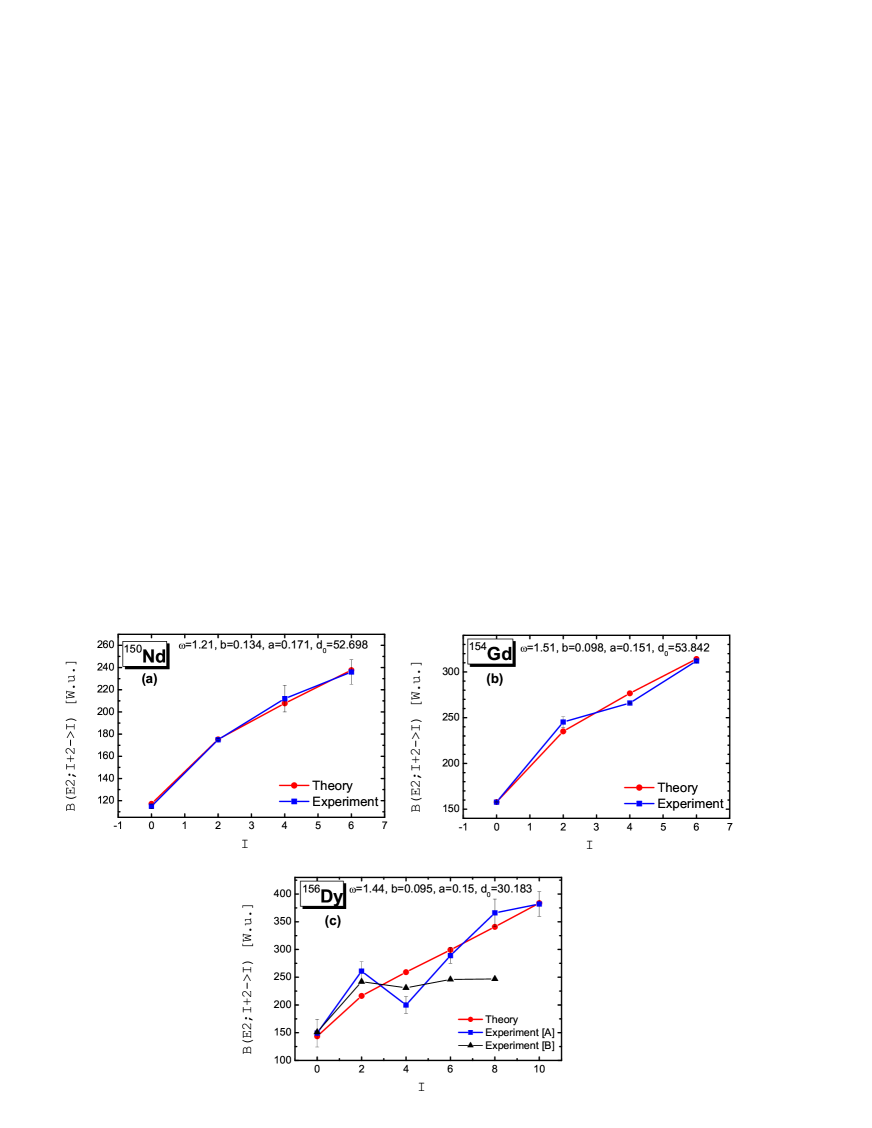
Figure 12: (Color online) Theoretical and experimental B(E2) transition probabilities (in W.u.) as functions of the angular momentum in the alternating parity spectra of ¹⁵⁰Nd, ¹⁵⁴Gd and ¹⁵⁶Dy. The data for ¹⁵⁰Nd, ¹⁵⁴Gd, and for Experiment[A] in ¹⁵⁶Dy are from [29]; Experiment[B] in ¹⁵⁶Dy is from [30]. The theoretical results are obtained by Eq. (49). See Sec. 5 for further discussion.

In the case of the infinite square well potential (case III), the model wave function is of the form

$$\Phi^{\pm}_{\nu,n,IM}(\eta,\,\phi)=c_{\nu,\,n}J_{\nu}(\kappa_{\nu,\,n}\eta)\sqrt{\frac{2I+1}{32\pi^{2}}}{D^{I}_{0,\,M}(\theta)}\varphi^{\pm}(\phi)\ ,$$ (54)

while the integrals over the variable $\eta$ read

$$S(E1,I_{i}\rightarrow I_{f})=\int_{0}^{\infty}d\eta J_{\nu_{i}}(\kappa_{\nu_{i},\,n_{i}}\eta)\eta^{3}J_{\nu_{f}}(\kappa_{\nu_{f},\,n_{f}}\eta)\ ;$$ (55)

$$S(EL,I_{i}\rightarrow I_{f})=\int_{0}^{\infty}d\eta J_{\nu_{i}}(\kappa_{\nu_{i},\,n_{i}}\eta)\eta^{2}J_{\nu_{f}}(\kappa_{\nu_{f},\,n_{f}}\eta).$$ (56)

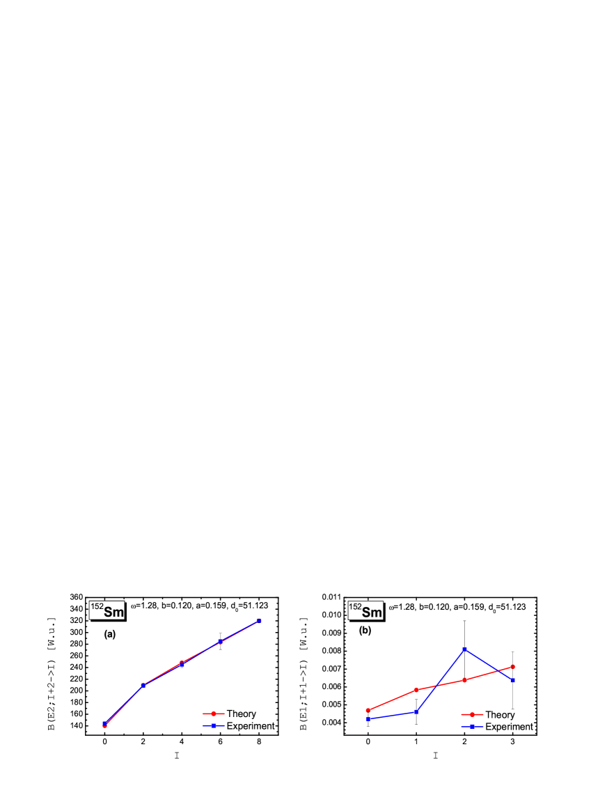
Figure 13: (Color online) Theoretical and experimental B(E2) [part (a)] and B(E1) [part (b)] transition probabilities (in W.u.) as functions of the angular momentum in the alternating parity spectrum of ¹⁵²Sm (data from [29]). The theoretical results are obtained by Eqs. (48) and (49).

In general, the above formalism can be applied for a detailed analysis of the electric transition rates in spectra where the collective quadrupole octupole dynamics carries the characteristics outlined in the cases I–III of our study. In Figs. 12 and 13 we illustrate its application to E2 transition probabilities in the nuclei ¹⁵⁰Nd, ¹⁵²Sm, ¹⁵⁴Gd, and ¹⁵⁶Dy, as well as to the E1 transitions in ¹⁵²Sm, in the framework of Case I. The results are obtained with the parameter sets given in Fig. 7. The quantity $a=\sqrt{BC}/\hbar$, appearing in Eqs. (52) and (53), has been considered as a fitting parameter. The constant $b_{1}$ in Eq. (48) has been determined so as to scale the theoretical $E1$ transition values with respect to the experimental data and takes the value $b_{1}=1.2\times 10^{-6}$, while the constants $b_{L}$ in Eq. (49) have been set equal to $1$.

We see a good agreement between theory and experiment for the B(E2) values in ¹⁵⁰Nd [Fig. 12(a)], ¹⁵²Sm [Fig. 13(a)], and ¹⁵⁴Gd [Fig. 12(b)]. In Fig. 12(c), the theoretical E2 transition probabilities in ¹⁵⁶Dy are compared to two different sets of experimental data, [29] and [30] (with no error bars reported in [30]). We see that the theoretical values follow only the overall increase of the experimental data. We should, however, remark that the two sets of data diverge essentially, especially at the higher angular momenta. There is also some discrepancy between theory and experiment in the E1 transition values in ¹⁵²Sm [Fig. 13(b)]. The results in Figs. 12(c) and 13(b) suggest that further examination of the formalism, as well as of the experimental data, may be necessary. The further analysis of data on electric transitions in a wider range of nuclei will be the subject of future work.

6 Influence of the $\gamma$ deformation mode on the $\beta_{2}$-$\beta_{3}$ collective motion

As it has been mentioned in Sec. 4, the present model framework does not include the $\gamma$ degree of freedom. Here we briefly discuss the possible ways in which this can be done and shortly estimate the influence of the $\gamma$ deformation mode on the collective motion in the $\beta_{2}$-$\beta_{3}$ space. The rotation energy of a system with presence of axial and triaxial quadrupole modes ($\beta_{2}$ and $\gamma$ ) and axial octupole degree of freedom ($\beta_{3}$) can be given by [13, 31]

$$\hat{T}_{\mbox{\scriptsize rot}}=\frac{1}{2}\sum_{i=1}^{3}\frac{\hat{I}_{i}^{2}}{J_{i}^{(2)}+J_{i}^{(3)}},$$ (57)

where

$$J_{i}^{(2)}=4B_{2}\beta_{2}^{2}\sin^{2}\left(\gamma-\frac{2\pi i}{3}\right),\qquad(i=1,2,3)$$ (58)

are the moment-of-inertia components of the quadrupole shape about the axes 1, 2 and 3, while those of the axially symmetric octupole shape are

$$J_{1}^{(3)}=J_{2}^{(3)}=6B_{3}\beta_{3}^{2},\qquad J_{3}^{(3)}=0.$$ (59)

A simple estimation of the $\gamma$- influence can be done by assuming small variations of the system around $\gamma=0$, as in the case of the X(5) model [12]. Then the quadrupole moment-of-inertia components (58) can be taken as

$$J_{1}^{(2)}=J_{2}^{(2)}=3B_{2}\beta_{2}^{2},\qquad J_{3}^{(2)}=4B_{2}\beta_{2}^{2}\sin^{2}\gamma.$$ (60)

As a result the rotation energy (57) obtains the form

$$\hat{T}_{\mbox{\scriptsize rot}}=\frac{1}{2}\left(\frac{\hat{I}^{2}-\hat{I}_{3}^{2}}{3B_{2}\beta_{2}^{2}+6B_{3}\beta_{3}^{2}}+\frac{\hat{I}_{3}^{2}}{4B_{2}\beta_{2}^{2}\sin^{2}\gamma}\right).$$ (61)

The first term in (61) corresponds to the centrifugal term in the quadrupole-octupole potential (2). The second term in (61) provides the influence of the $\gamma$ mode on the potential. After taking into account Eq. (61) with $d_{2}=3B_{2}$ and $d_{3}=6B_{3}$, and by including a $\gamma$- oscillation term, the potential (2) can be generalized in the form

$$U(\beta_{2},\beta_{3},\gamma,I)=\frac{1}{2}C_{2}{\beta_{2}}^{2}+\frac{1}{2}C_{3}{\beta_{3}}^{2}+\frac{1}{2}C^{\prime}_{2}{\gamma}^{2}+\frac{X(I)-K^{2}/2}{d_{2}\beta_{2}^{2}+d_{3}\beta_{3}^{2}}+\frac{3K^{2}/2}{4d_{2}\beta_{2}^{2}\sin^{2}\gamma},$$ (62)

where $K$ is the projection of the angular momentum on the body-fixed $z$-axis. Then for a fixed value of $\gamma$ the extremum conditions (3) and (4) in Sec. 2 provide the following cases for the bottom of the potential (62) in the $\beta_{2}$-$\beta_{3}$ space.

1) $\beta_{3\mbox{\scriptsize min}}=0$ with

$$\beta_{2\mbox{\scriptsize min}}=\pm\left\{\frac{2}{d_{2}C_{2}}\left[X(I)+\frac{K^{2}}{2}\left(\frac{3}{4\sin^{2}\gamma}-1\right)\right]\right\}^{1/4}.$$ (63)

2) $\beta_{2\mbox{\scriptsize min}}\neq 0$ and $\beta_{3\mbox{\scriptsize min}}\neq 0$ with the condition

$$C_{2}=\frac{[2X(I)-K^{2}]d_{2}}{(d_{2}\beta_{2\mbox{\scriptsize min}}^{2}+d_{3}\beta_{3\mbox{\scriptsize min}}^{2})^{2}}+\frac{3K^{2}}{4d_{2}\beta_{2\mbox{\scriptsize min}}^{4}\sin^{2}\gamma}\ \ \mbox{and}\ \ C_{3}=\frac{[2X(I)-K^{2}]d_{3}}{(d_{2}\beta_{2\mbox{\scriptsize min}}^{2}+d_{3}\beta_{3\mbox{\scriptsize min}}^{2})^{2}}\ .$$ (64)

The following comments can be done on the above result.

i) The appearance of $\beta_{2}^{2}$ in the denominator of the second term in (62) divides the $\beta_{2}$-$\beta_{3}$ space into two half-spaces, $\beta_{2}>0$ and $\beta_{2}<0$, separated by an infinite potential barrier at $\beta_{2}=0$. For this reason the potential minimum with $\beta_{2\mbox{\scriptsize min}}=0$ and $\beta_{3\mbox{\scriptsize min}}\neq 0$ does not appear.

ii) Eqs. (63) and (64) illustrate the ways in which the term involving the $\gamma$ deformation mode can shift the position of the potential minima in the $\beta_{2}$-$\beta_{3}$ space (compare with cases i)–iii) including Eq. (5) in Sec. 2). Note that for $K=0$ the influence of the $\gamma$ mode on the $\beta_{2}$-$\beta_{3}$ potential shape automatically disappears. This is a limit in which the $\beta_{2}$ and $\gamma$ degrees of freedom are weakly coupled and can be adiabatically separated, which is implied in the framework of the present work. The involvement of the $K=2$ configurations in the collective motion implies the consideration of a strong $\beta_{2}$-$\gamma$ coupling [32].

iii) The involvement of the $\gamma$ degree of freedom in the above way would influence the correlation between the axial $\beta_{2}$ and $\beta_{3}$ variables due to the appearance of the second term in $C_{2}$ [Eq. (64)], as a consequence of the last term in the potential (62). Now, in terms of the polar variables, the potential will depend on both $\eta$ and $\phi$, so that the variables in the Schrödinger equation cannot be directly separated. This could be done in a way similar to the adiabatic separation of the $\beta$ and $\gamma$ degrees of freedom in the X(5) model framework [12], as well as in the framework of the AQOA model [33]. Alternatively, the problem could be solved numerically in a way similar to the approach of Ref. [32].

A more general way to examine the influence of the $\gamma$ deformation mode on the quadrupole-octupole motion of the system could be based on the complete form (58) of the quadrupole moment-of-inertia components, so that the $\gamma$ variable would not be limited in the vicinity of zero. Furthermore, non-axiality of the octupole degree of freedom can be considered. Any efforts in these directions should be based on numerical solution of the problem.

7 Summary and conclusions

The present study outlines some dynamical properties of a system with simultaneously manifesting quadrupole and octupole degrees of freedom. We remark that the obtained results represent a restricted class of exact analytic solutions of the problem. This is due to the correlation (18) between the mass and the inertial parameters, which essentially simplifies the Hamiltonian (11) in the form of Eq. (19). In addition, the correlation (6) between the inertial and oscillator parameters brings the potential in a form depending on the “effective deformation” variable $\eta$ only, and not on the relative “angular” variable $\phi$, thus allowing an exact separation of variables in the Schrödinger equation. As it is explained in Sec. 4, the above correlations provide a coherent interplay between the quadrupole and octupole collective modes. In this respect, the presently considered potentials suggest some specific properties of quadrupole–octupole collectivity, which can be developed in various nuclear regions.

However, despite the above limitations (the necessary price we pay for solving the problem exactly) we were able to identify a region of nuclei where the assumed “equal” presence of quadrupole and octupole degrees of freedom can take place in the collective motion. We found that the structure of the spectrum in the case of the potential (12), illustrated in Fig. 6, is similar to the structure of alternating parity bands in some rare earth nuclei. On this basis, we have reproduced quite accurately the energy levels and the staggering patterns in the nuclei ¹⁵⁰Nd, ¹⁵²Sm, ¹⁵⁴Gd, and ¹⁵⁶Dy, as demonstrated in Figs. 7 and 8. In these spectra the reduction of the staggering amplitude indicates the trend of forming octupole deformations towards the higher angular momenta. However, the slow decrease of the parity effect does not allow this to happen at reasonable (observed) angular momenta. The B(E2) transition probabilities have been also described with a reasonable accuracy (Figs. 12 and 13), while the result for B(E1) transition probabilities in ¹⁵²Sm [Fig. 13(b)] suggests further tests of the formalism and analysis of additional experimental data.

We remark that the energy expression (25) cannot reproduce the complicated beat staggering effects observed in the octupole bands of light actinide nuclei [34]. The latter have been described [14], with good accuracy, by the use of the Quadrupole–Octupole Rotation Model [35]. Thus, compared to the light actinide region, the application of expression (25) indicates a different behavior of the quadrupole–octupole collectivity in the rare earth nuclei, with a less developed octupole deformation and a more strongly pronounced octupole vibration mode. The present analysis suggests that in this case the coherent (equal) contribution of quadrupole and octupole oscillations can take place in the collective motion of nuclei.

The potentials with fixed energy minima (cases II and III) can be related generally to a situation in which the vibrational and rotational degrees of freedom are weakly coupled. Then the rotational angular momentum slightly affects the quadrupole-octupole vibration motion, which suggests a constant (or nearly constant) behavior of the staggering amplitude. In particular this is well seen in the case II.B, where the direct contribution of the rotational motion is excluded. Thus, the spectrum illustrated in Fig. 10 suggests an essentially quadrupole-octupole vibrational motion of the system. Cases II.A and III, in which the rotational mode is taken into account, suggest quadrupole-octupole vibrations with an adiabatically manifested rotational motion. We remark that the constant staggering patterns, illustrated in Figs. 9 and 10, are in some meaning idealistic cases, as far as the current experimental data do not show such a strong persistence of the parity effect at high angular momenta. On the other hand, the square well potential of case III appears to be applicable to examining the possible critical behavior of the quadrupole–octupole collectivity in different nuclear regions. Studies in this direction have been implemented recently in the light actinide nuclei [33]. We suggest that further analysis of experimental data for quadrupole–octupole spectra would be of use for testing the prediction of the staggering pattern illustrated in Fig. 11 for the case of the square well potential (17).

It is important to note that the present exactly solvable model can be naturally extended, beyond the “coherent interplay” assumption, to a more general non-analytic problem in the following two ways. First, we can release the correlation (6) between the inertial and oscillator parameters, allowing the potential to depend on the variable $\phi$. Then the problem can still be transformed into a form having an analytical solution, by performing an “approximate” separation of variables, as done in [33] and in the framework of the X(5) symmetry model [12]. The second extension would be to release the correlation (18) between the mass and inertial parameters. This would allow us to examine different ways in which the coupled quadrupole and octupole degrees of freedom enter the collective motion. In this case, however, more sophisticated mathematical and numerical techniques have to be sought to solve the problem.

Finally, we also remark that the developed formalism contains several limits. Thus, when the quadrupole variable is frozen to some stable quadrupole deformation, the potentials and the spectra of the cases I-III transform to the respective ones appearing in the one-dimensional problem [14, 15]. Another interesting limit can be obtained by appropriate parameter values, for which the difference $\Delta k^{2}$ is negligible compared to $\widetilde{X}(I)$ for all angular momentum values. Then the staggering effect vanishes, and the odd and even angular momentum sequences appear in a single non-perturbed collective band. For example, if such a transition is performed in case III, the spectrum presented in Fig. 11 is reduced to the structure supposed to correspond to the transition between octupole vibrations and stable octupole deformation, in which a single octupole band is formed [33]. It is also of interest to take into account the non-axiality of the quadrupole and/or the octupole degree of freedom, in order to examine how the present results are modified. Studies in these directions will be the subject of further work.

Acknowledgments

We thank Prof. P. G. Bizzeti and Prof. R. V. Jolos for valuable discussions and comments. This work is supported by DFG and by the Bulgarian Scientific Fund under contract F-1502/05.

References

- [1] A. Bohr and B. R. Mottelson, Nuclear Structure, vol. II (Benjamin, New York, 1975).
- [2] I. Ahmad and P. A. Butler, Annu. Rev. Nucl. Part. Sci. 43, 71 (1993).
- [3] P. A. Butler and W. Nazarewicz, Rev. Mod. Phys. 68, 349 (1996).
- [4] H. J. Krappe and U. Wille, Nucl. Phys. A 124, 641 (1969).
- [5] G. A. Leander, R. K. Sheline, P. Möller, P. Olanders, I. Ragnarsson, and A. J. Sierk, Nucl. Phys. A 388, 452 (1982).
- [6] R. Jolos, P. von Brentano, and F. Dönau, J. Phys. G 19, L151 (1993).
- [7] R. Jolos, P. von Brentano, Phys. Rev. C 49, R2301 (1994).
- [8] A. Ya. Dzyublik and V. Yu. Denisov, Yad. Fiz. 56, 30 (1993) [Phys. At. Nucl. 56, 303 (1993)].
- [9] V. Yu. Denisov and A. Ya. Dzyublik, Nucl. Phys. A 589, 17 (1995).
- [10] R. F. Casten and N. V. Zamfir, Phys. Rev. Lett. 87, 052503 (2001).
- [11] R. M. Clark, M. Cromaz, M. A. Deleplanque, M. Descovich, R. M. Diamond, P. Fallon, R. B. Fierstone, I. Y. Lee, A. O. Macchiavelli, H. Mahmud, E. Rodriguez-Vieitez, F. S. Stephens, and D. Ward, Phys. Rev. C 68, 037301 (2003).
- [12] F. Iachello, Phys. Rev. Lett. 87, 052502 (2001).
- [13] J. P. Davidson, Collective Models of the Nucleus (Academic Press, New York, 1968).
- [14] N. Minkov, S. Drenska, P. Yotov, and W. Scheid, J. Phys. G: Nucl. Part. Phys. 32, 497 (2006).
- [15] P. G. Bizzeti and A. M. Bizzeti-Sona, Phys. Rev. C 70, 064319 (2004).
- [16] P. M. Davidson, Proc. R. Soc. London Ser. A 135, 459 (1932).
- [17] J. P. Elliott, J. A. Evans, and P. Park, Phys. Lett. B 169, 309 (1986).
- [18] D. J. Rowe and C. Bahri, J. Phys. A 31, 4947 (1998).
- [19] E. der Mateosian and J. K. Tuli, Nucl. Data Sheets 75, 827 (1995).
- [20] A. Artna-Cohen, Nucl. Data Sheets 79, 1 (1996).
- [21] C. W. Reich and R. G. Helmer, Nucl. Data Sheets 85, 171 (1998).
- [22] C. W. Reich, Nucl. Data Sheets 99, 753 (2003).
- [23] J. Eisenberg and W. Greiner, Nuclear Theory, vol. I Nuclear Models (North-Holland, Amsterdam, 1970).
- [24] C. Dorso, W. Myers and W. Swiatecki, Nucl. Phys. A 451, 189 (1986).
- [25] W. Myers and W. Swiatecki, Nucl. Phys. A 531, 93 (1991).
- [26] V. Yu. Denisov, Yad. Fiz. 49, 644 (1989) [Sov. J. Nucl. Phys. 49, 399 (1989)].
- [27] V. Yu. Denisov, Yad. Fiz. 55, 2647 (1992) [Sov. J. Nucl. Phys. 55, 1478 (1992)].
- [28] A. R. Edmonds, Angular Momentum in Quantum Mechanics (Princeton University Press, Princeton, 1957).
- [29] http://www.nndc.bnl.gov/ensdf/.
- [30] A. Dewald, O. Möller, D. Tonev, A. Fitzler, B. Saha, K. Jessen, S. Heinze, A. Linnemann, J. Jolie, K. O. Zell, P. von Brentano, P. Petkov, R. F. Casten, M. Caprio, J. R. Cooper, R. Krücken, V. Zamfir, D. Bazzacco, S. Lunardi, C. Rossi Alvarez, F. Brandolini, C. Ur, G. de Angelis, D. R. Napoli, E. Farnea, N. Marginean, T. Martinez, and M. Axiotis, Eur. Phys. J. A 20, 173 (2004).
- [31] V. M. Maslov, Yu. V. Porodzinskij, N. A. Tetereva, M. Baba, and A. Hasegawa, Nucl. Phys. A 764, 212 (2006).
- [32] M. A. Caprio, Phys. Rev. C 72, 054323 (2005).
- [33] D. Bonatsos, D. Lenis, N. Minkov, D. Petrellis, and P. Yotov, Phys. Rev. C 71, 064309 (2005).
- [34] D. Bonatsos, C. Daskaloyannis, S. Drenska, N. Karoussos, N. Minkov, P. Raychev and R. Roussev, Phys. Rev. C 62, 024301 (2000).
- [35] N. Minkov, S. Drenska, P. Raychev, R. Roussev and D. Bonatsos, Phys. Rev. C 63, 044305 (2001).