Physical Origin of Density Dependent Force of the Skyrme Type within the Quark Meson Coupling Model

Abstract

A density dependent, effective nucleon-nucleon force of the Skyrme type is derived from the quark-meson coupling model – a self-consistent, relativistic quark level description of nuclear matter. This new formulation requires no assumption that the mean scalar field is small and hence constitutes a significant advance over earlier work. The similarity of the effective interaction to the widely used SkM^∗ force encourages us to apply it to a wide range of nuclear problems, beginning with the binding energies and charge distributions of doubly magic nuclei. Finding acceptable results in this conventional arena, we apply the same effective interaction, within the Hartree-Fock-Bogoliubov approach, to the properties of nuclei far from stability. The resulting two neutron drip lines and shell quenching are quite satisfactory. Finally, we apply the relativistic formulation to the properties of dense nuclear matter in anticipation of future application to the properties of neutron stars.

I Introduction

Given that QCD is almost universally believed to be the fundamental theory of the strong interaction, one of the great challenges facing modern nuclear physics is to derive the properties of atomic nuclei from it. Amongst the hopes for a more fundamental description of nuclear matter is to be able to extrapolate to extreme regions of density, asymmetry or even strangeness with rather more confidence than has hitherto been possible. One might also expect to understand the nuclear EMC effect Geesaman:1995yd ; Cloet:2005rt ; Smith:2005ra and a number of other challenges to traditional nuclear theory Saito:2005rv ; Strauch:2002wu .

While at the present time there has only been exploratory work aimed at relating QCD itself to nuclear structure Thomas:2004iw ; Chanfray:2005sa , there has been considerably more work within the framework of quark models and effective field theories utilizing the symmetries of QCD. Here we shall concentrate on one particular model, the Quark-Meson Coupling (QMC) model Guichon:1987jp ; Guichon:1995ue ; Saito:1995up ; Saito:2005rv , which is built around the self-consistent response of the relativistic, confined valence quarks to the Lorentz scalar mean field in nuclear matter. In previous work Guichon:2004xg we have shown that the main features of the effective interactions used in nuclear physics can be quantitatively derived from the QMC model. In order to do this we rewrote the QMC model as an equivalent, effective Hamiltonian with zero range many body interactions. The many body character of the interactions was a direct consequence of the response of the quark structure to the nuclear environment. We found that this Hamiltonian was in quite good agreement with the popular Skyrme-III interaction Vautherin:1971aw , which led us to conclude that quark level dynamics does play a key role in ordinary nuclear physics, even if it can be hidden within an effective many-body theory.

However, one unsatisfactory feature of the derivation in Ref. Guichon:2004xg was that the approximations which were required meant that one could not justify the use of the resulting effective Hamiltonian much beyond the density of ordinary nuclear matter – $(\rho_{0}=0.16$fm${}^{-3})$. One of those approximations is actually tied to the physics of the model: the response of the quark structure to the nuclear medium leads to a non-linear meson field equation which is intractable in its full generality. In Ref. Guichon:2004xg we relied on an iterative solution of the field equations, which essentially amounted to an expansion in powers of the density. We showed that this is an acceptable approximation for ordinary nuclear densities, with the medium effects then appearing as many body forces. Another approximation used in that work was a non-relativistic expansion which, in the framework of the iterative solution, appeared unavoidable. The latter approximation was also motivated by our wish to compare the effective Hamiltonian with the Skyrme interaction which is a non-relativistic object. These approximations, which were justified in the context of the earlier work, become untenable at higher densities. For instance, in this model one finds that the velocity of sound exceeds the velocity of light at about $3\rho_{0}.$ This is somewhat frustrating because it prevents us applying the model to the study of neutron stars.

In this work we propose a new formulation which does not rely on the approximations which we have just outlined. Instead of solving the meson field equation iteratively, we expand the field around its nuclear expectation value and treat the deviation as a perturbation. This leads to an effective Hamiltonian with a density dependent two-body force. As the equation for the expectation value can be solved exactly (at least in a numerical sense), the bulk of the medium effects may be taken into account without any assumption about the value of the density. This is a major advance with respect to the formulation in Ref. Guichon:2004xg . Moreover, the case of uniform nuclear matter, which is the relevant approximation for neutron stars, can now be treated in a way consistent with relativity.

This paper is organized as follows. In Section II we recall the basic elements of the QMC model. This is followed in Section III by the formal derivation of the equivalent, density dependent NN force. A non-relativistic reduction of the full effective interaction is carried out in Section IV in order to make a detailed comparison with the density dependent Skyrme force in SectionV. In Section VI we carry out a full Hartree-Fock calculation with the non-relativistic, effective force that we derived and compare the results for selected finite nuclei against experimental data. Finally, in Section VII we solve the full model for uniform matter containing just nucleons – leaving for future work the generalization of the method to include hyperons. Section VIII presents some concluding remarks and suggestions for further work.

II The QMC model

In the Quark Meson Coupling model, the nuclear system is represented as a collection of confined clusters of three valence quarks. Because it is possible to carry through much of the calculation analytically, the MIT bag model was chosen to confine the quarks. It is assumed that the effect of having these bags overlap, that is clusters of more than three quarks, can be neglected. This approximation certainly breaks down at some density but we assume that it is still acceptable in the density range that we consider. In this respect, we observe that the bag model is an effective realisation of confinement, which must not be taken too literally. Indeed, QCD lattice simulations Alexandrou:2002sn ; Bissey:2005sk strongly suggest that the true picture is closer to a Y-shaped color string attached to the quarks. Outside this relatively thin string one has the ordinary, non-perturbative QCD vacuum where the quarks from the other nucleons can pass without disturbing the structure. Thus, while the bag model imposes a strict boundary condition which prevents the quarks from travelling through its boundary, this must be seen as the average representation of a more complex situation. One should not attribute a deep physical meaning to the boundary of the cavity nor to its size. In particular, estimating the density at which the non-overlap approximation breaks down as $\rho=1/V$, with $V$ the bag volume, is certainly too pessimistic.

The salient feature of the QMC model is that the interactions are generated by the exchange of mesons coupled locally to the quarks. In a literal interpretation of the bag model, where only quarks and gluons can live inside the cavity, this coupling would be unnatural. On the other hand, in terms of the more realistic picture presented by lattice QCD, the quarks are attached to a string but otherwise move in the non-perturbative QCD vacuum. There nothing prevents them from feeling the vacuum fluctuations which we describe by meson fields. As in our earlier work, we limit our considerations to the $\sigma,\,\omega$ and $\rho$ mesons. We recall that the $\sigma$ meson here is not the chiral partner of the pion. It is a chiral invariant field which represents correlated two-pion exchange. The quarks of the bag are in the Weinberg representation Thomas:1981ps ; Thomas:1982kv , where the mass term $\bar{q}q$ is a chiral scalar which allows a chiral invariant coupling of the form $\sigma\bar{q}q$.

Of course, this is not the end of the story because the transformation to the Weinberg representation introduces an infinite set of derivative pion-quark couplings. These produce a complicated set of multi-pion exchanges, together with contact interactions. We assume, in the spirit of both Quantum Hadrodynamics Serot:1984ey and the one boson exchange model, that the bulk of the corresponding physics can be modeled by the $\sigma,\,\omega$ and $\rho$ exchanges between quarks. It is clear that the long ranged single pion exchange does not fit in this picture and must be treated separately. However, because of its pseudoscalar nature, this exchange does not contribute to the mean nuclear field. In the Hartree Fock approximation , which will be our framework in the following, it contributes through its exchange (Fock) term. This effect has been estimated in the framework of infinite nuclear matter and found to be small. More exactly, most of the effect can be absorbed by a readjustment of the couplings to the other mesons. This is our first motivation for neglecting this part of the interaction but we must keep in mind that the argument is only true in the Hartree Fock approximation. When other nucleon correlations are taken into account, the game changes but this is beyond the scope of this work.

Our starting point is the classical energy of a system of non-overlapping bags of quarks, which are coupled to the nuclear meson fields $\sigma,\,\omega$ and $\rho$. Following Ref. Guichon:2004xg we can write

$$E=\sum_{i}\left(\sqrt{P_{i}^{2}+M_{eff}(\sigma)^{2}}+g_{\omega}\omega+V_{so}\right)+E_{mesons}\,,$$ (1)

where the first term is the relativistic energy of nucleon $i$, with momentum $P_{i}$ and effective mass $M_{eff}$, $g_{\omega}\omega$ is the repulsion felt by each nucleon as a result of its vector interaction with the time component of the $\omega$ mean field, $V_{so}$ is the spin-orbit potential and the static meson energy is

$$E_{mesons}=\frac{1}{2}\int d\vec{r}\left[\left(\nabla\sigma\right)^{2}+m_{\sigma}^{2}\sigma^{2}\right]-\frac{1}{2}\int d\vec{r}\left[\left(\nabla\omega\right)^{2}+m_{\omega}^{2}\omega^{2}\right]\,,$$ (2)

with $m_{\sigma},m_{\omega},m_{\rho}$ the meson masses. As usual, we consider only the time component of the vector fields. The effect of the $\rho$, which can be treated by analogy with the $\omega$ field, will be introduced at the end. The expression for the spin orbit interaction, $V_{so}$, first derived in Ref. Guichon:1995ue , is not necessary at this stage.

The effective mass, $M_{eff}(\sigma)$, is the rest frame energy of a quark bag in the $\sigma$ field of the medium, evaluated at the center of the bag. In order to calculate $M_{eff}(\sigma)$ one needs to solve the bag equations for the relevant value of the $\sigma$ field. However, we have checked that a quadratic expansion:

$$M_{eff}(\sigma)=M-g_{\sigma}\sigma+\frac{d}{2}\left(g_{\sigma}\sigma\right)^{2}$$ (3)

is accurate up to values of $g_{\sigma}\sigma$ as large as 600MeV, which corresponds to densities far beyond the physical limitations of the model. The parameter $d$ is the scalar polarizability of the nucleon. It depends explicitly on the response of the quark structure to the external scalar field. In the bag model it is well represented as a function of the bag radius, $R_{B}$, as

$$d=0.0044+0.211R_{B}-0.0357R_{B}^{2}\,,$$ (4)

where both $d$ and $R_{B}$ are in fm. This does not give exactly the values that were used in Ref. Guichon:2004xg , because we have now included the contribution of the spin dependent, “hyperfine” color interaction to the bag energy. The coupling constant, $g_{\sigma}$, which by definition refers to the nucleon, is related to the $\sigma$–quark coupling, $g_{\sigma}^{q}$, by

$$g_{\sigma}=3g_{\sigma}^{q}\int_{Bag}d\vec{r}\,\bar{q}q(\vec{r})\,,$$ (5)

where $q$ is the valence quark wavefunction for the free bag. For the vector couplings the relationship is

$$g_{\omega}=3g_{\omega}^{q},\,g_{\rho}=g_{\rho}^{q}.$$ (6)

Equation (3) holds for any flavor, $f$, of hadrons, provided the couplings and scalar polarizability are replaced by their corresponding values $g_{\sigma}(f),d(f)$. In the bag model they are related to $g_{\sigma}$ and $d$ in a well defined way. Thus the treatment of flavors other than the nucleon is straightforward and does not introduce new parameters. This matter will be developed in forthcoming work. Here we limit our consideration to the case where the medium contains just clusters with the quantum numbers of protons and neutrons.

III Hamiltonian

By hypothesis, the meson fields are time independent. Therefore the classical Hamiltonian for the nuclear system is simply

$$H(R_{i},P_{i})=E(R_{i},P_{i},\sigma\to\sigma_{sol},\omega\to\omega_{sol})\,,$$ (7)

where $R_{i}$ and $P_{i}$ are the position and momentum of nucleon $i$ and $\sigma_{sol},\omega_{sol}$ are the the solutions of the equations of motion corresponding to Eq. (1)

$$\frac{\delta E}{\delta\sigma}=\frac{\delta E}{\delta\omega}=0$$

that is

$$-\nabla^{2}\sigma+m_{\sigma}^{2}\sigma = -\sum_{i}\delta(\vec{r}-\vec{R}_{i})\frac{\partial}{\partial\sigma}\sqrt{P_{i}^{2}+M_{eff}(\sigma)^{2}},$$ (8)

$$-\nabla^{2}\omega+m_{\sigma}^{2}\omega = g_{\omega}\sum_{i}\delta(\vec{r}-\vec{R}_{i})\,.$$ (9)

Note that in Eqs. (8,9) we have neglected the contribution corresponding to the variation of the spin orbit interaction $V_{so}$. As pointed out in Ref. Guichon:2004xg , this results in an error of order $V_{so}^{2}$ in the Hamiltonian and it is consistent to neglect it because the spin-orbit interaction in Eq. (1) has been derived as a first order perturbation Guichon:1995ue . Since the equation for the $\omega$ field is linear, its solution is elementary and poses no new problem with respect to our previous work. Its contribution to the energy will be written later and we now concentrate on the field equation for the $\sigma$.

We assume that it makes sense to write

$$\sigma=<\sigma>+\delta\sigma\,,$$

where the C-number $<\sigma>$, also written $\bar{\sigma}$, denotes the nuclear ground state expectation value, that is

$$<\sigma(\vec{r})>=\int d\vec{R}_{1}...d\vec{R}_{A}\Phi^{*}(\vec{R}_{1}...\vec{R}_{A})\sigma(\vec{r},\vec{R}_{i},\vec{P}_{i})\Phi(\vec{R}_{1}...\vec{R}_{A})$$

and to consider the deviation, $\delta\sigma$, as a small quantity. If we define

$$K=\sum_{i}\delta(\vec{r}-\vec{R}_{i})\sqrt{P_{i}^{2}+M_{eff}(\sigma)^{2}}\,,$$ (10)

we see that the $\sigma$ field equation has the form

$$\left(-\nabla^{2}+m_{\sigma}^{2}\right)\left(\bar{\sigma}+\delta\sigma\right)=-\frac{\partial K}{\partial\sigma}=-\frac{\partial K}{\partial\sigma}(\bar{\sigma})-\delta\sigma\frac{\partial^{2}K}{\partial\sigma^{2}}(\bar{\sigma})-\cdots$$ (11)

We also expand $\frac{\partial K}{\partial\sigma}(\bar{\sigma}),\frac{\partial^{2}K}{\partial\sigma^{2}}(\bar{\sigma})$ about their expectation values

$$\frac{\partial K}{\partial\sigma}(\bar{\sigma}) = <\frac{\partial K}{\partial\sigma}(\bar{\sigma})>+\delta\left[\frac{\partial K}{\partial\sigma}(\bar{\sigma})\right]\,,$$

$$\frac{\partial^{2}K}{\partial\sigma^{2}}(\bar{\sigma}) = <\frac{\partial^{2}K}{\partial\sigma^{2}}(\bar{\sigma})>+\delta\left[\frac{\partial^{2}K}{\partial\sigma^{2}}(\bar{\sigma})\right]\,,$$ (12)

and suppose that

$$\delta\sigma,\,\delta\left[\frac{\partial K}{\partial\sigma}(\bar{\sigma})\right],\,\delta\left[\frac{\partial^{2}K}{\partial\sigma^{2}}(\bar{\sigma})\right]$$

are small quantities. We can then solve the meson field equation order by order, which gives:

$$\left(-\nabla^{2}+m_{\sigma}^{2}\right)\bar{\sigma} = -<\frac{\partial K}{\partial\sigma}(\bar{\sigma})>$$ (13)

$$\left(-\nabla^{2}+m_{\sigma}^{2}\right)\delta\sigma = -\delta\left[\frac{\partial K}{\partial\sigma}(\bar{\sigma})\right]-\delta\sigma<\frac{\partial^{2}K}{\partial\sigma^{2}}(\bar{\sigma})>\,,$$ (14)

$$= -\frac{\partial K}{\partial\sigma}(\bar{\sigma})+<\frac{\partial K}{\partial\sigma}(\bar{\sigma})>-\delta\sigma<\frac{\partial^{2}K}{\partial\sigma^{2}}(\bar{\sigma})>\,.$$

As we limit the expansion of the Hamiltonian to order $(\delta\sigma)^{2},$ it is sufficient to solve the field equation at order $\delta\sigma$, which corresponds to Eqs. (13,14). Using integration by parts, the Hamiltonian (1) may be expanded as

$$H = \int d\vec{r}\left.K\right|_{\bar{\sigma}}+\delta\sigma\frac{\partial K}{\partial\sigma}(\bar{\sigma})+\frac{1}{2}(\delta\sigma)^{2}\frac{\partial^{2}K}{\partial\sigma^{2}}(\bar{\sigma})$$ (15)

$$+\frac{1}{2}\bar{\sigma}\left(-\nabla^{2}+m_{\sigma}^{2}\right)\bar{\sigma}+\delta\sigma\left(-\nabla^{2}+m_{\sigma}^{2}\right)\bar{\sigma}+\frac{1}{2}\delta\sigma\left(-\nabla^{2}+m_{\sigma}^{2}\right)\delta\sigma\,.$$

To this order we can replace

$$\frac{\partial^{2}K}{\partial\sigma^{2}}(\bar{\sigma})\to<\frac{\partial^{2}K}{\partial\sigma^{2}}(\bar{\sigma})>$$

because this multiplies $(\delta\sigma)^{2}$. Using Eqs. (13,14) we then find:

$$H=\int d\vec{r}\,\left[K(\bar{\sigma})-\frac{1}{2}\bar{\sigma}<\frac{\partial K}{\partial\sigma}(\bar{\sigma})>+\frac{1}{2}\delta\sigma\left(\frac{\partial K}{\partial\sigma}(\bar{\sigma})-<\frac{\partial K}{\partial\sigma}(\bar{\sigma})>\right)\right].$$ (16)

Note that the mean field approximation amounts to neglecting $\delta\sigma$ in Eq.(16). To complete the derivation we need a prescription for writing the quantum form of $K$ and its derivatives. The important simplification is that these are one body operators because they are evaluated at the C-number point $\sigma=\bar{\sigma}$. Thus we can write

$$K(\bar{\sigma})=\sum_{\alpha\beta}K_{\alpha\beta}(\bar{\sigma})a_{\alpha}^{\dagger}a_{\beta}\,,$$

where $a_{\alpha}^{\dagger},a_{\alpha}$ are the creation and destruction operators for the complete 1-body basis $|\alpha>$. The matrix elements $K_{\alpha\beta}(\bar{\sigma})$ must be chosen so as to reproduce the classical limit, Eq.(10). In the momentum space representation, there is a natural choice

$$K(\bar{\sigma})=\frac{1}{2V}\sum_{\vec{k},\vec{k}^{\prime}}e^{i(\vec{k}-\vec{k}^{\prime}).\vec{r}}\left(\sqrt{k^{2}+M_{eff}[\bar{\sigma}(\vec{r})]^{2}}+\sqrt{k^{\prime 2}+M_{eff}[\bar{\sigma}(\vec{r})]^{2}}\right)a_{\vec{k}}^{\dagger}a_{\vec{k}^{\prime}}\,,$$ (17)

where the symmetrization is introduced to guaranty hemiticity and $V$ is the normalisation volume. We also choose

$$\frac{\partial K}{\partial\sigma}(\bar{\sigma})=\frac{1}{2V}\sum_{\vec{k},\vec{k}^{\prime}}e^{i(\vec{k}-\vec{k}^{\prime}).\vec{r}}\frac{\partial}{\partial\bar{\sigma}}\left(\sqrt{k^{2}+M_{eff}[\bar{\sigma}(\vec{r})]^{2}}+\sqrt{k^{\prime 2}+M_{eff}[\bar{\sigma}(\vec{r})]^{2}}\right)a_{\vec{k}}^{\dagger}a_{\vec{k}^{\prime}}\,,$$ (18)

with a similar expression for the second derivative. The ordering ambiguities associated with products of non-commuting operators are fixed by the normal ordering prescription, which amounts to removing that part of the energy which originates from the interaction of one nucleon with its own field.

The Hamiltoniam defined in Eq. (16) is not a standard many-body problem, since we do not know $\bar{\sigma}$ and $\delta\sigma$ until the ground state nuclear wave function has been specified. Therefore the Hamiltonian must be determined (through $\bar{\sigma}$ and $\delta\sigma$ ) at each step of the self consistent procedure. This is a significant technical complication. On the other hand, for our purposes it is not necessary to solve this Hamiltonian in the general case. One of our main goals is to obtain the equation of state for very dense nuclear matter, with a view to applying it to neutron stars Lawley:2006ps , but in this case we only need the uniform matter approximation for which the model is easy to solve. Of course, we do need to consider finite size effects for ordinary nuclei, a necessary step in order to show that the model is realistic with respect to nuclear phenomenology. However, in this case, we can make a non-relativistic expansion and build a density functional, $<H(\vec{r})>$, which can then be used in variational calculations of nuclei.

IV Non relativistic expansion

We first consider the case of finite nuclei, in order to verify that the model is indeed realistic. For this purpose we build the density functional, $<H(\vec{r})>$, using approximations which are standard in low energy nuclear physics. The approximations that we use below involve a non-relativistic expansion and the neglect of those velocity dependent and finite range forces which involve more than 2 bodies – as is the case for conventional effective nuclear forces. This amounts to expanding the terms which involve either the momentum or the gradient of the density in powers of the $\sigma$ nucleon coupling and stopping at order $g_{\sigma}^{2}$. To simplify the expressions we omit the spin and flavor indices as long as they are not truly necessary. We first define the number density, $D(\vec{r})$, and kinetic density, $\xi(\vec{r})$, by

$$D(\vec{r})=\frac{1}{V}\sum_{\vec{k},\vec{k}^{\prime}}e^{i(\vec{k}-\vec{k}^{\prime}).\vec{r}}a_{\vec{k}}^{\dagger}a_{\vec{k}^{\prime}},\,\,\,\,\xi(\vec{r})=\frac{1}{V}\sum_{\vec{k},\vec{k}^{\prime}}e^{i(\vec{k}-\vec{k}^{\prime}).\vec{r}}\frac{k^{2}+k^{\prime 2}}{2}a_{\vec{k}}^{\dagger}a_{\vec{k}^{\prime}}.$$ (19)

Then, following the approximation scheme defined above and using Eq. (3) we find the following expression for the operator $K$ and its derivatives

$$\left.K\right|_{\bar{\sigma}} = D(\vec{r})M_{eff}[\bar{\sigma}(\vec{r})]+\frac{\xi(\vec{r})}{2M}\left(1+\frac{g_{\sigma}\bar{\sigma}}{M}\right)\,,$$

$$\left.\frac{\partial K}{\partial\sigma}\right|_{\bar{\sigma}} = D(\vec{r})\frac{\partial M_{eff}}{\partial\bar{\sigma}}+g_{\sigma}\frac{\xi(\vec{r})}{2M^{2}}\,,$$ (20)

$$\left.\frac{\partial^{2}K}{\partial\sigma^{2}}\right|_{\bar{\sigma}} = dg_{\sigma}^{2}D(\vec{r})\,.$$

Substituting these expression into Eqs. (13,14) and using the same approximations, we can solve for $\bar{\sigma}$ and $\delta\sigma$:

$$g_{\sigma}\bar{\sigma}=\frac{G_{\sigma}<D>}{1+dG_{\sigma}<D>}-G_{\sigma}\frac{<\xi>}{2M^{2}}+G_{\sigma}\frac{\nabla^{2}<D>}{m_{\sigma}^{2}}\,,$$ (21)

$$\delta\sigma=\frac{1}{\tilde{m}_{\sigma}^{2}}\left(-\frac{\partial K}{\partial\sigma}(\bar{\sigma})+<\frac{\partial K}{\partial\sigma}(\bar{\sigma})>\right)+\frac{1}{\tilde{m}_{\sigma}^{2}}\nabla^{2}\frac{1}{\tilde{m}_{\sigma}^{2}}\left(-\frac{\partial K}{\partial\sigma}(\bar{\sigma})+<\frac{\partial K}{\partial\sigma}(\bar{\sigma})>\right)\,,$$ (22)

where we have defined $G_{\sigma}=g_{\sigma}^{2}/m_{\sigma}^{2}$ and the (position dependent) effective $\sigma$ mass

$$\tilde{m}_{\sigma}^{2}=m_{\sigma}^{2}\left(1+G_{\sigma}d<D>\right)\,.$$ (23)

We can now substitute Eqs. (20,21,22) into Eq. (16) to obtain the Hamiltonian of the model. In practice we want the corresponding density functional in the Hartree Fock approximation, so we need to evaluate (note that by definition $<\delta\sigma>=0)$

$$<H(\vec{r})> = <K(\bar{\sigma})>-\frac{1}{2}\bar{\sigma}<\frac{\partial K}{\partial\sigma}(\bar{\sigma})>+\frac{1}{2}<\delta\sigma\frac{\partial K}{\partial\sigma}(\bar{\sigma})>\,,$$ (24)

where the ground state wave function is a Slater determinant, with Fermi level $F$, built from the single particle wave functions $\Phi^{j}(\vec{r},\sigma,m)$. We now restore the spin flavor dependence but restrict our considerations to nuclei made of protons and neutrons. So the flavor index is just the isospin projection $m=\pm 1/2.$ As usual, we define Vautherin:1971aw  :

$$\rho_{m}(\vec{r}) = \sum_{i\in F}\sum_{\sigma}\left|\Phi^{i}(\vec{r},\sigma,m)\right|^{2},\,\,\,\,\rho(\vec{r})=\sum_{m}\rho_{m}(\vec{r})\,,$$ (25)

$$\tau_{m}(\vec{r}) = \sum_{i\in F}\sum_{\sigma}\left|\vec{\nabla}\Phi^{i*}(\vec{r},\sigma,mo)\right|^{2},\,\,\,\,\tau(\vec{r})=\sum_{m}\tau_{m}(\vec{r})\,,$$ (26)

$$\vec{J}_{m}(\vec{r}) = i\,\sum_{i\in F}\sum_{\sigma\sigma^{\prime}}\vec{\sigma}_{\sigma^{\prime}\sigma}\times\left[\vec{\nabla}\Phi^{i}(\vec{r},\sigma,m)\right]\Phi^{i*}(\vec{r},\sigma^{\prime},m),\,\,\,\,\vec{J}(\vec{r})=\sum_{m}\vec{J}_{m}(\vec{r})\,,$$ (27)

and using standard techniques we find, after some algebra:

$$<H(\vec{r})> = \rho M+\frac{\tau}{2M}$$ (28)

$$+\frac{G_{\sigma}}{2M^{2}}\left(\rho\tau+\frac{1}{8}\sum_{m}\rho_{m}\nabla^{2}\rho_{m}\right)$$

$$-\left(\frac{G_{\sigma}}{2m_{\sigma}^{2}}+\frac{G_{\sigma}}{4M^{2}}\right)\left(\rho\nabla^{2}\rho-\sum_{m}\left(\frac{1}{4}\rho_{m}\nabla^{2}\rho_{m}-\rho_{m}\tau_{m}\right)\right)$$

$$-\frac{1}{2}\frac{G_{\sigma}}{1+dG_{\sigma}\rho}\left(\rho^{2}-\frac{1}{2(1+dG_{\sigma}\rho)^{2}}\sum_{m}\rho_{m}^{2}\right)\,.$$

For completeness, we give the $\omega,\rho$ and spin orbit contributions (labelled $IS$ for isoscalar and $IV$ for isovector):

$$<:{\cal H}_{so}^{IS}(\vec{r}):> = -\frac{1}{4M^{2}}\left[G_{\sigma}+\left(2\frac{\mu_{IS}}{\mu_{N}}-1\right)G_{\omega}\right]\sum_{mm^{\prime}}\left[\left(1+\frac{1}{2}\delta_{mm^{\prime}}\right)\rho_{m^{\prime}}\vec{\nabla}.\vec{J}_{m^{\prime}}\right]\,,$$ (29)

$$<:{\cal H}_{so}^{IV}(\vec{r}):> = -\frac{G_{\rho}}{4M^{2}}\left[2\frac{\mu_{IV}}{\mu_{N}}-1\right]\sum_{mm^{\prime}}\left[\left(mm^{\prime}+\frac{1}{2}C_{mm^{\prime}}\right)\rho_{m^{\prime}}\vec{\nabla}.\vec{J}_{m}\right]\,,$$ (30)

$$<:{\cal H}_{\omega}(\vec{r}):> = \frac{G_{\omega}}{2}\sum_{mm^{\prime}}\left[\left(1-\frac{1}{2}\delta_{mm^{\prime}}\right)\rho_{m}\rho_{m^{\prime}}\right.$$ (31)

$$\left.+\frac{1}{m_{\omega}^{2}}\left(\rho_{m}\nabla^{2}\rho_{m^{\prime}}-\frac{1}{4}\delta_{mm^{\prime}}\left(\rho_{m}\nabla^{2}\rho_{m}-4\rho_{m}\tau_{m}\right)\right)\right]\,,$$

$$<:{\cal H}_{\rho}(\vec{r}):> = \frac{G_{\rho}}{2}\sum_{mm^{\prime}}\left\{\left(mm^{\prime}-\frac{1}{2}C_{mm^{\prime}}\right)\rho_{m}\rho_{m^{\prime}}\right.$$ (32)

$$\left.+\frac{1}{m_{\rho}^{2}}\left(mm^{\prime}-\frac{1}{4}C_{mm^{\prime}}\right)\rho_{m}\nabla^{2}\rho_{m^{\prime}}+\frac{1}{m_{\rho}^{2}}C_{mm^{\prime}}\rho_{m}\tau_{m^{\prime}}\right\}\,,$$

where: $C_{mm^{\prime}}=\delta_{mm^{\prime}}m^{2}+(\delta_{m,m^{\prime}+1}+\delta_{m^{\prime},m+1})/2$ and $G_{\omega}=g_{\omega}^{2}/m_{\omega}^{2},G_{\rho}=g_{\rho}^{2}/m_{\rho}^{2}.$ The isoscalar and isovector magnetic moments which appear in the spin orbit interaction have the values

$$\mu_{IS}=\mu_{p}+\mu_{n}=0.88,\,\,\mu_{IV}=\mu_{p}-\mu_{n}=4.7\,.$$ (33)

As we have already pointed out, these expressions are the same as in our previous work. We note that all terms which involve the square of the spin density, $\vec{J}$, have been neglected. This is common practice and, since it amounts to treating the spin orbit interaction as a first order perturbation, it is consistent with our derivation of the expression for the effective mass, Eq. (1).

It is convenient to have a more explicit expression for the density functional. Using Eqs. (28 – 32) one can write, using the same notation as in Ref. Chabanat:1997un :

$$<H(\vec{r})>=\rho M+\frac{\tau}{2M}+{\cal H}_{0}+{\cal H}_{3}+{\cal H}_{eff}+{\cal H}_{fin}+{\cal H}_{so}\,,$$ (34)

where

$${\cal H}_{0}+{\cal H}_{3} = {\rho}^{2}\,\left[\frac{-3\,{G_{\rho}}}{32}+\frac{{G_{\sigma}}}{8\,{\left(1+d\,\rho\,{G_{\sigma}}\right)}^{3}}-\frac{{G_{\sigma}}}{2\,\left(1+d\,\rho\,{G_{\sigma}}\right)}+\frac{3\,{G_{\omega}}}{8}\right]+$$ (36)

$${\left({{\rho}_{n}}-{{\rho}_{p}}\right)}^{2}\left[\frac{5\,{G_{\rho}}}{32}+\frac{{G_{\sigma}}}{8\,{\left(1+d\,\rho\,{G_{\sigma}}\right)}^{3}}-\frac{{G_{\omega}}}{8}\right],$$

$${\cal H}_{eff} = \left[\left(\frac{{G_{\rho}}}{8\,{m_{\rho}}^{2}}-\frac{{G_{\sigma}}}{2\,{m_{\sigma}}^{2}}+\frac{{G_{\omega}}}{2\,{m_{\omega}}^{2}}+\frac{{G_{\sigma}}}{4\,{M_{N}}^{2}}\right)\,{{\rho}_{n}}+\left(\frac{{G_{\rho}}}{4\,{m_{\rho}}^{2}}+\frac{{G_{\sigma}}}{2\,{M_{N}}^{2}}\right)\,{{\rho}_{p}}\right]\,{{\tau}_{n}}$$ (37)

$$+p\leftrightarrow n,$$

$${\cal H}_{fin} = \left[\left(\frac{3\,{G_{\rho}}}{32\,{m_{\rho}}^{2}}-\frac{3\,{G_{\sigma}}}{8\,{m_{\sigma}}^{2}}+\frac{3\,{G_{\omega}}}{8\,{m_{\omega}}^{2}}-\frac{{G_{\sigma}}}{8\,{M_{N}}^{2}}\right)\,{{\rho}_{n}}\right.$$ (39)

$$+\left.\left(\frac{-3\,{G_{\rho}}}{16\,{m_{\rho}}^{2}}-\frac{{G_{\sigma}}}{2\,{m_{\sigma}}^{2}}+\frac{{G_{\omega}}}{2\,{m_{\omega}}^{2}}-\frac{{G_{\sigma}}}{4\,{M_{N}}^{2}}\right)\,{{\rho}_{p}}\right]{{\nabla}^{2}}({{\rho}_{n}})+p\leftrightarrow n,$$

$${\cal H}_{so} = \nabla\cdot{J_{n}}\left[\left(\frac{-3\,{G_{\sigma}}}{8\,{M_{N}}^{2}}-\frac{3\,{G_{\omega}}\,\left(-1+2\,{{\mu}_{s}}\right)}{8\,{M_{N}}^{2}}-\frac{3\,{G_{\rho}}\,\left(-1+2\,{{\mu}_{v}}\right)}{32\,{M_{N}}^{2}}\right)\,{{\rho}_{n}}\right.$$ (41)

$$+\left.\left(\frac{-{G_{\sigma}}}{4\,{M_{N}}^{2}}+\frac{{G_{\omega}}\,\left(1-2\,{{\mu}_{s}}\right)}{4\,{M_{N}}^{2}}\right)\,{{\rho}_{p}}\right]+p\leftrightarrow n.$$

We have determined the couplings $G_{\sigma},\,G_{\omega},\,G_{\rho}$ by fixing the saturation density and binding energy of normal nuclear matter to be $\rho_{0}=0.16$fm³ and $E_{B}=-15.85$ MeV, as well as the asymmetry energy of nuclear matter as $a_{4}=30$ MeV. Apart from a small readjustment of the couplings, we found no significant sensitivity to the bag radius. We therefore display our results for only one value, $R_{B}=0.8$fm, which is quite realistic Thomas:1982kv . The $\omega$ and $\rho$ masses are set at their experimental values. The last parameter, which is not well fixed by experiment, is the $\sigma$ mass. We shall use $m_{\sigma}=600,650,700,750MeV.$ The corresponding results are given in Table 1. We see that the incompressibility, $K_{N}$, is a little high with respect to the currently prefered range, but we point out that this calculation has not yet taken into account the single pion exchange interaction. We know Guichon:2004xg that the pion Fock term alone reduces $K_{N}$ by as much as 10% and it is likely that this is amplified by other correlations.

$m_{\sigma}$(MeV)	$G_{\sigma}$(fm${}^{2})$	$G_{\omega}$(fm${}^{2})$	$G_{\rho}$(fm${}^{2})$	$K_{N}$(MeV)
600	12.652	9.838	9.67	346
650	12.428	9.308	8.583	346
700	12.254	8.899	7.724	346
750	12.116	8.575	7.048	346

Table 1: The couplings $G_{\sigma},G_{\omega},G_{\rho}$ for a bag radius $R_{B}=0.8$fm and several values of the scalar meson mass, $m_{\sigma}$. The last column is the nuclear incompressibility.

V Comparison with the Skyrme force

As a means of orientation, we compare the density functional of our model with that corresponding to a typical density-dependent effective interaction. We choose to compare with the popular Skyrme SkM^∗ parametrisation rather than more recent ones, such Sly4 Chabanat:1997un , because in the latter case the formal identification is complicated by the larger number of parameters. The SkM^∗ interaction depends on 6 parameters: $t_{0},t_{1},t_{2},t_{3},x_{0}$ and $W_{0}$ and its energy density Chabanat:1997un may be written, using the same notation as in the previous section:

$${\cal H}_{0}+{\cal H}_{3} = \frac{{\rho}^{\frac{1}{6}}\,{t_{3}}\,\left(2\,{\rho}^{2}-{{\rho}_{n}}^{2}-{{\rho}_{p}}^{2}\right)}{24}+\frac{{t_{0}}\,\left({\rho}^{2}\,\left(2+{x_{0}}\right)-\left(1+2\,{x_{0}}\right)\,\left({{\rho}_{n}}^{2}+{{\rho}_{p}}^{2}\right)\right)}{4}\,,$$ (42)

$${\cal H}_{eff} = \frac{\rho\,\tau\,\left(2\,{t_{1}}+2\,{t_{2}}\right)}{8}+\frac{\left(-{t_{1}}+{t_{2}}\right)\,\left({{\rho}_{n}}\,{{\tau}_{n}}+{{\rho}_{p}}\,{{\tau}_{p}}\right)}{8}\,,$$ (43)

$${\cal H}_{fin} = \frac{-\left(\rho\,\left(6\,{t_{1}}-2\,{t_{2}}\right)\,{{\nabla}^{2}}(\rho)\right)}{32}+\frac{\left(3\,{t_{1}}+{t_{2}}\right)\,\left({{\rho}_{n}}\,{{\nabla}^{2}}({{\rho}_{n}})+{{\rho}_{p}}\,{{\nabla}^{2}}({{\rho}_{p}})\right)}{32}\,,$$ (44)

$${\cal H}_{so} = \frac{-\left({W_{0}}\,\left(\rho\,\nabla\cdot J+\nabla\cdot{J_{n}}\,{{\rho}_{n}}+\nabla\cdot{J_{p}}\,{{\rho}_{p}}\right)\right)}{2}\,,$$ (45)

To simplify, we compare ${\cal H}_{eff},{\cal H}_{fin}$ and ${\cal H}_{so}$ with the QMC expressions Eqs. (37,39,41), in the case $N=Z.$ This detemines $t_{1},t_{2}$ and $W_{0}$. To find $t_{0},t_{3}$ and $x_{0}$, we consider the term ${\cal H}_{0}+{\cal H}_{3}$. As the functional form is not the same, we fit $\left({\cal H}_{0}+{\cal H}_{3}\right)_{QMC}$ with the form which appears in $\left({\cal H}_{0}+{\cal H}_{3}\right)_{SkM}$ in the range $\rho\in[0\to 0.2$ fm${}^{-3}]$. We first do this in the case $N=Z$, which determines $t_{0}$ and $t_{3}$ and using these values we do the fit for $Z/A=92/208$, which determines $x_{0}.$ The results are collected in Table 2 for several values of the $\sigma$ mass. We find satisfactory agreement with the SkM^∗ parameters in the window $m_{\sigma}=650\div 700$ MeV. This comparison suggests that our model may provide an acceptable representation of low energy nuclear physics.

However, this comparison is really rather qualitative. First, we have minimized the isospin effects by setting $N=Z$ when determining the parameters $t_{1},t_{2},W_{0}$. Second, the values we find for $t_{0}$ and $t_{3}$ depend somewhat on the range of density we use for the fit. Thus a more direct comparison of our model with actual nuclear data is desirable. This is done in the next section.

$m_{\sigma}$(MeV)	$t_{0}$(fm${}^{2})$	$t_{1}$(fm${}^{4})$	$t_{2}$(fm${}^{4})$	$t_{3}$(fm${}^{5/2})$	$x_{0}$	$W_{0}$(fm${}^{4})$	Deviation
600	-12.72	2.64	-1.12	74.25	0.17	0.6	33%
650	-12.48	2.21	-0.77	71.73	0.13	0.56	18%
700	-12.31	1.88	-0.49	69.8	0.1	0.53	18%
750	-12.18	1.62	-0.28	68.28	0.08	0.51	38%
SkM∗	-13.4	2.08	-0.68	79	0.09	0.66	0%

Table 2: Comparison of the SkM^∗ parameters with the QMC predictions for several values of $m_{\sigma}.$

VI Hartree Fock calculations for finite nuclei

As pointed out in the previous section, the QMC and the Skyrme energy functionals have a similar structure. However, the density and the isospin dependence of some terms, particularly $H_{3}$ and $H_{so}$, are rather different in the two approaches. Thus, for the Skyrme functionals the term $H_{3}$ has a density dependence of the form $\rho^{\alpha}$. Originally this term was interpreted as having been generated by a three-body contact interaction, which is equivalent to a two-body density-dependent force in even-even nuclei Vautherin:1971aw . In the QMC functional, the density dependence of $H_{3}$ is much more complicated. However, a more complicated density dependence could also appears in Skyrme type energy functionals if they are derived from a more fundamental theory based on G-matrix, such as density-matrix expansion (DME) method of Negele and Vautherin Negele72 . A comparison between the energy functionals corresponding to DME and to standard Skyrme forces shows that in fact the strength of the density-dependent term is rather similar in both cases, in spite of their different density dependence. It is interesting to observe that a density dependence of a fractional type, as appears in QMC, was previously considered in phenomenological functionals by Fayans et al. fayans . The advantage of fractional expressions in particle density is that the corresponding energy functional preserves causal behaviour up to very high densities. This is actually the case for the QMC functional as well.

Another difference between the QMC and standard Skyrme energy functionals arises in the isospin dependence of the spin-orbit term $H_{so}$. In both cases the form factor of the one-body spin-orbit interaction for a nucleon with the isospin $m$ ($n$ or $p$) can be written as:

$$W_{m}(r)=a\nabla\rho_{m}+b\nabla\rho_{\tilde{m}}\,,$$ (46)

where $\rho_{m}$ is the particle density, while $\tilde{m}$ denotes the opposite isospin to $m$. For the standard Skyrme forces the ratio $s=a/b$ is equal to 2. This isospin dependence of the one-body spin-orbit potential is induced by the exchange term (since the Skyrme two-body spin-orbit force is isospin independent). For the QMC functional used in the calculations below, the ratio $s$ is about 2.78. This strong isospin dependence in both the QMC and Skyrme functionals is in contrast with the weak isospin dependence employed in the relativistic mean field models, in which the contribution of Fock (exchange) terms is neglected ring .

Starting from the QMC energy functional one can easily derive the corresponding Hartree-Fock (HF) equations. They have a form similar to the Skyrme-HF equations, apart from the rearrangement term and the one-body spin-orbit interaction, which (as discussed above) have a different density and isospin dependence. The HF equations were solved in coordinate space, following the method described in Ref. Vautherin:1971aw and the Coulomb interaction was treated in a standard way – i.e., the contribution of its exchange part was calculated in the Slater approximation. The calculations were performed for the doubly magic nuclei ¹⁶O, ⁴⁰Ca, ⁴⁸Ca and ²⁰⁸Pb. For definiteness, the $\sigma$ meson mass has been set to $m_{\sigma}$=700MeV, as suggested by the comparison with the SkM^∗ interaction. At this point we recall that the QMC model is essentially classical because both the position and velocity of the bag are assumed known in the energy expression (3). The quantization then leaves some arbitrariness in the ordering of the momentum dependent pieces of the interaction. As pointed out in previous work Guichon:2004xg , in the non-relativistic approximation the difference between the orderings is equivalent to a change of about 10% in $m_{\sigma}$. In this work the ordering is fixed by the relativistic expression chosen for the operator $K$, Eq. (17). The non-relativistic reduction then leads to an ordering which is not the same as in Ref. Guichon:2004xg . This is why the $\sigma$ meson mass that we use here is somewhat higher. Note that this ordering ambiguity is only of concern in the case of finite nuclei. In uniform matter, which is the relevant approximation for neutron stars, the problem does not exist.

The results for the binding energies and charge radii are shown in Table 3. The charge densities are calculated with the proton form factor usually employed in the Skyrme-HF calculations Vautherin:1971aw . From Table 3 one can see that QMC-HF gives results which are in reasonable agreement with the experimental values. The agreement is not as good as that given by the recent Skyrme or RMF models, but one should keep in mind that in these models the experimental values for the binding energies and radii are included in the fitting procedure, which is not the case for the QMC functional.

One also finds a similarly reasonable description for the spin-orbit splittings, shown in Table 4. Since the isospin dependence in QMC-HF is stronger than in Skyrme-HF, one would expect different values for nuclei with large isospin asymetry. However, as can be seen from Table 4, the differences are rather small. This is primarily because the spin-orbit splitting depends on the product of the spin-orbit form factor and the corresponding single-particle wave functions. Thus, if the wave functions are not strongly localised in the surface region, where $W_{\tau}(r)$ is effective, the influence of the isospin dependence of $W_{\tau}(r)$ upon the splitting need not be so significant.

In Figs. 1, 2 we show the proton and neutron densities calculated with the QMC model and with the Sly4 Skyrme force Chabanat:1997un . In the proton case we also show the experimental values DeJager:1987qc . Once again the two models give rather similar results, with the largest differences noticed for the neutron skin of ²⁰⁸Pb. More precisely, for this nucleus the neutron skin (i.e., the difference between the neutron and proton rms radii) is equal to 0.12fm for QMC, compared to 0.16fm for the Skyrme force. With respect to experiment the QMC model tends to overestimate the density in the central region, but the overall agreement is quite good, given that the model has no parameter adjusted to fit the properties of finite nuclei.

Next we analyse the predictions of the QMC functional in nuclei far from stability. In order to do such a study, one must take into account the contribution of pairing correlations. They are treated here in the Hartree-Fock-Bogoliubov (HFB) approach. For the pairing interaction we have taken a density-dependent contact interaction of the form bertsch :

$$V=V_{0}\left[1-\eta\left(\frac{\rho}{\rho_{0}}\right)^{\alpha}\right]\delta(r_{1}-r_{2})\,.$$ (47)

With this pairing force the QMC-HFB equations are local. They have been solved in coordinate space by truncating the quasiparticle spectrum at an energy equal to 60 MeV. The parameters of the pairing force have been fixed to the values: $V_{0}=-333$ MeV fm^-3, $\eta=0.5$, $\alpha=1$, and $\rho_{0}=0.16$fm^-3, which were chosen to yield a reasonable average gap for the tin isotopes ( a benchmark for pairing models).

With this force we have investigated the position of the drip lines, which give the limits for bound nuclear systems. Here we present the results for the two-neutron drip line predicted by the QMC functional for Ni and Zr isotopes. The two-neutron drip line is defined by the value of N (number of neutrons) for which the two-neutron separation energy becomes negative. In the QMC-HFB calculations the neutron drip line appears around N=60 for Ni and around N=82 for Zr. These positions of the drip line are similar to the predictions provided by the Skyrme force SLy4, commonly used in non-relativistic calculations Chabanat:1997un .

Another important property which characterizes nuclei far from stability is the shell quenching, which has important consequences for the astrophysical rapid capture processes. The phenomenological energy functionals show that when one approaches the drip line the shell gaps associated with the magic numbers of neutrons or protons are quenched in comparison with stable nuclei. The shell quenching can be tested by calculating the two-neutron separation energies, $S_{2n}$, across a magic number. Here we present the QMC-HFB results for the neutron magic number N=28. The variation of $S_{2n}$ across N=28 is calculated for two extreme values of proton numbers, namely Z=32 (proton drip-line region) and Z=14 (neutron drip-line region). One thus finds that $S_{2n}$ changes by about 8 MeV for Z=32 and by about 2-3 MeV for Z=14. This strong shell quenching is very close to that obtained in the Skyrme-HFB calculations (see Fig. 15 of Ref. Chabanat:1997un ).

In conclusion, the QMC functional gives a reasonable description of the known double magic nuclei and predicts, for nuclei far from stability, similar properties to those found in mean field Skyrme models.

	$E_{B}$ (MeV, exp)	$E_{B}$ (MeV, QMC)	$r_{c}$ (fm, exp)	$r_{c}$ (fm, QMC)
${}^{16}O$	7.976	7.618	2.73	2.702
${}^{40}Ca$	8.551	8.213	3.485	3.415
${}^{48}Ca$	8.666	8.343	3.484	3.468
${}^{208}Pb$	7.867	7.515	5.5	5.42

Table 3: Binding energy and radii calculated in QMC-HF, as described in the text.

	Neutrons (exp)	Neutrons (QMC)	Protons (exp)	Protons (QMC)
${}^{16}O,\,1p_{1/2}-1p_{3/2}$	6.10	6.01	6.3	5.9
${}^{40}Ca,\,1d_{3/2}-1d_{5/2}$	6.15	6.41	6.00	6.24
${}^{48}Ca,\,1d_{3/2}-1d_{5/2}$	6.05 (Sly4)	5.64	6.06 (Sly4)	5.59
${}^{208}Pb,\,2d_{3/2}-2d_{5/2}$	2.15 (Sly4)	2.04	1.87 (Sly4)	1.74

Table 4: Comparison between the QMC and “experimental” spin orbit splittings. Because the experimental splittings are no so well known in the case of ${}^{48}Ca$ and ${}^{208}Pb$, we give the values corresponding to the Skyrme Sly4 prediction.

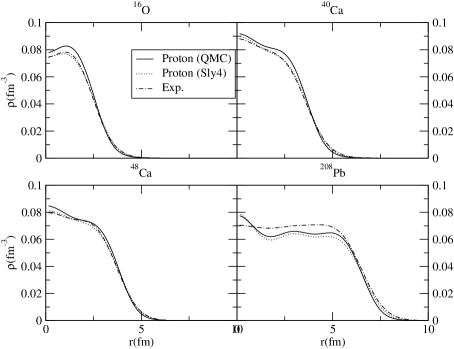
Figure 1: Proton densities of the QMC model compared with experiment and the prediction of the Skyrme Sly4 force.

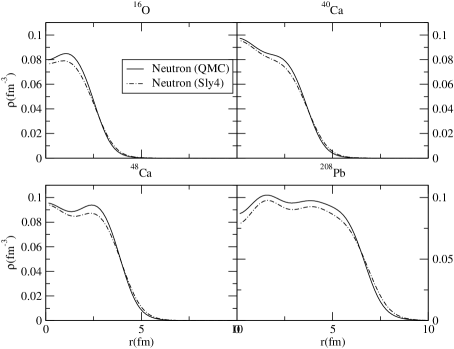
Figure 2: Neutron densities of the QMC model compared with the prediction of the Skyrme Sly4 force.

VII High density uniform matter

In the previous section we have shown that the non-relativistic approximation to the Hamiltonian developed in section III gives an acceptable phenomenology for ordinary nuclei. This give us some confidence to examine the consequences of the model in the high density region, relevant to the neutron star problem. The classical application of a density dependent force of the Skyrme type to this problem was that of Negele and Vautherin Negele:1971vb . Of course, all non-relativistic effective theories must break down as the density increases and we therefore concentrate on a truly relativistic treatment in this case. For neutron stars one can restrict consideration to uniform nuclear matter, which implies that $<K(\bar{\sigma})>$ and its derivatives are numbers independent of $\vec{r.}$ The constant expectation value of the sigma field $\bar{\sigma}$ is then determined by the self consistent equation (see Eq. (13)):

$$\bar{\sigma}=-\frac{1}{m_{\sigma}^{2}}<\frac{\partial K}{\partial\sigma}(\bar{\sigma})>\,,$$ (48)

which is solved numerically. The fluctuation, $\delta\bar{\sigma}$, is given by Eq. (14), where the effective $\sigma$ mass, $\tilde{m}_{\sigma}$, is now constant and the solution, expressed in terms of the $\sigma$-meson Green function, ${\cal G}_{\sigma}$, is

$$\delta\sigma(\vec{r}) = \int d\vec{r}^{\prime}{\cal G}_{\sigma}(\vec{r}-\vec{r}^{\prime})\left(-\frac{\partial K}{\partial\sigma}(\bar{\sigma},\vec{r}^{\prime})+<\frac{\partial K}{\partial\sigma}(\bar{\sigma})>\right)$$ (49)

$$= \int d\vec{r}^{\prime}\frac{d\vec{q}}{(2\pi)^{3}}\frac{e^{i\vec{q}.(\vec{r}-\vec{r}^{\prime})}}{q^{2}+\tilde{m}_{\sigma}^{2}}\left(-\frac{\partial K}{\partial\sigma}(\bar{\sigma},\vec{r}^{\prime})+<\frac{\partial K}{\partial\sigma}(\bar{\sigma})>\right)$$

Note that, even though $\bar{\sigma}$ is constant, the operator $K$ and its derivative have an explicit dependence on position (see Eqs. (17,18)) which disappears only in the expectation value.

For uniform matter the energy density is

$$\epsilon=\frac{<H>}{V}=\frac{1}{V}\int d\vec{r}\,\left[<K(\bar{\sigma})>-\frac{1}{2}\bar{\sigma}<\frac{\partial K}{\partial\sigma}(\bar{\sigma})>+\frac{1}{2}<\delta\sigma(\vec{r})\,\frac{\partial K}{\partial\sigma}(\bar{\sigma},\vec{r})>\right]\,.$$ (50)

In a Fermi gas we have

$$<K_{m}(\bar{\sigma})>=\frac{2}{(2\pi)^{3})}\int_{o}^{k_{F}(m)}d\vec{k}\sqrt{k^{2}+M^{2}(\bar{\sigma})},\,\,\,\,<K(\bar{\sigma})>=\sum_{m}<K_{m}(\bar{\sigma})>\,,$$ (51)

with $k_{F}(m)$ the Fermi level of the isospin species $m.$ Using the solution for $\delta\sigma$ we get, using standard techniques :

$$\frac{<H>}{V} = <K(\bar{\sigma})>+\frac{1}{2m_{\sigma}^{2}}\left(<\frac{\partial K}{\partial\sigma}(\bar{\sigma})>\right)^{2}$$ (52)

$$+ \frac{1}{(2\pi)^{6}}\sum_{f}\int_{0}^{k_{F}(m)}d\vec{k}_{1}d\vec{k}_{2}\frac{1}{(\vec{k}_{1}-\vec{k}_{2})^{2}+\tilde{m}_{\sigma}^{2}}\frac{\partial}{\partial\bar{\sigma}}\sqrt{k_{1}^{2}+M^{2}(\bar{\sigma})}\frac{\partial}{\partial\bar{\sigma}}\sqrt{k_{2}^{2}+M^{2}(\bar{\sigma})}.$$

Finally we must add the contributions $<V_{\omega}>,<V_{\rho}>$ associated with $\omega$ and $\rho$ exchange. However, since these interactions are purely 2-body there is nothing new with respect to our previous calculation. One finds

$$\frac{<V_{\omega}>}{V} = \frac{G_{\omega}}{2}\rho^{2}-G_{\omega}\sum_{m}\frac{1}{(2\pi)^{6}}\int_{0}^{k_{F}(m)}d\vec{k}_{1}d\vec{k}_{2}\frac{m_{\omega}^{2}}{(\vec{k}_{1}-\vec{k}_{2})^{2}+m_{\omega}^{2}},$$ (53)

$$\frac{<V_{\rho}>}{V} = \frac{G_{\rho}}{8}\left(\rho_{p}-\rho_{n}\right)^{2}-G_{\rho}\sum_{mm^{\prime}}C_{mm^{\prime}}\frac{1}{(2\pi)^{6}}\int_{0}^{k_{F}(m)}d\vec{k}_{1}\int_{0}^{k_{F}(m^{\prime})}d\vec{k}_{2}\frac{m_{\rho}^{2}}{(\vec{k}_{1}-\vec{k}_{2})^{2}+m_{\rho}^{2}}.$$ (54)

The energy density (52,53,54) and its non-relativistic version, given in Section IV, correspond to the same model. However, as in any theory, the parameters depend on the approximation scheme and therefore we need to readjust the couplings $G_{\sigma},G_{\omega},G_{\rho}$ to reproduce the saturation properties for normal nuclear matter. We do this for $R_{B}=0.8$fm and $m_{\sigma}=700MeV$. As can be seen in Table 5, the couplings we get are significantly different from those obtained with the non-relativistic expansion. The most important effect arises from the non-relativistic approximation (21) to the self consistentency equation (48) for $\bar{\sigma}$. If we were to use the same coupling constants in both equations, we would find a value of $\bar{\sigma}$ which, at the saturation point, differs by 15%.

	$G_{\sigma}$(fm${}^{2})$	$G_{\omega}$(fm${}^{2})$	$G_{\rho}$(fm${}^{2})$	$K_{N}$(MeV)
Non relativistic	12.254	8.899	7.724	346
Relativistic	11.334	7.274	4.56	342

Table 5: The couplings $G_{\sigma},G_{\omega},G_{\rho}$ of the non-relativistic (first line) and the relativistic (second line) version of the model for $R_{B}=0.8$fm and the $m_{\sigma}=700MeV$

In Fig. 3 we show the binding energy $E_{B}$, pressure $P$, incompressibility $K_{N}$ and sound velocity $V_{s}$ of symmetric nuclear matter predicted by our model (QMC) and the Skyrme (SkM^∗) interaction. We recall the definitions:

$$E_{B}=\frac{\epsilon}{\rho}-M,\ P=\rho^{2}\frac{\partial E_{B}}{\partial\rho},\ K_{N}=9\frac{\partial P}{\partial\rho},\ V_{s}=\sqrt{\frac{\rho K}{9(\epsilon+P)}}\,.$$ (55)

As we have restricted the flavor composition to protons and neutrons, the curves must not be taken too seriously for densities above $2\div 3$ times $\rho_{0}$, because there the appearance of hyperons is expected to become important. However, the comparison between QMC and SkM^∗ is still meaningful. One sees that the behavior of the two models is qualitatively similar in the range of densities displayed in the plots. Of course, at much higher density the SkM^∗ model would violate the causality limit $(V_{s}=1)$, because of its non-relativistic nature. By contrast the QMC model, because of its relativistic formulation, gives $V_{s}<1$ at any density. The QMC binding energy curve is stiffer than that for SkM^∗. This is not unexpected in view of the high value of $K_{N}(\rho_{0})$ given by QMC. However, the difference is not spectacular when one considers the full density range. This is even more obvious when one looks at the incompressibility curve as a function of density. In fact the curves cross somewhere above $\rho=1$fm^-3.

The situation changes radically when one considers the case of neutron matter – as shown in Fig. 4. The QMC equation of state is considerably stiffer than that for SkM^∗ above $\rho\sim 0.2$fm${}^{-3}.$ This difference is not too surprising because in the Skyrme interaction the isospin dependence appears only in the 2-body interaction through the $x_{0}$ parameter, while in the QMC model it is also generated by the non-linearity of the $\sigma$ field equation, as can be seen in Eq.(36) . Thus one may expect that the neutron stars predicted by the QMC model will have higher maximum masses than in the SkM^∗ model. However one cannot draw firm conclusions until the effect of hyperons has been calculated.

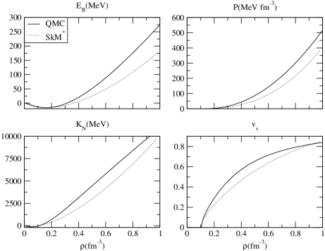
Figure 3: Comparison of the QMC and SkM^∗ model for symmetric matter.

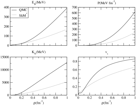
Figure 4: Comparison of the QMC and SkM^∗ model for neutron matter.

VIII Conclusion

Starting from the QMC model, we have derived a density dependent effective nucleon-nucleon force which is not limited to low density. The application of this effective interaction to the properties of doubly magic nuclei and then to nuclei far from stability yields results in quite acceptable agreement with popular effective forces which are far more phenomenological and which have rather more parameters. This provides one with confidence in the underlying physical concepts of the QMC model, most notably the scalar polarizability of a hadron which results from the self-consistent response of the confined valence quarks to the mean scalar field in the medium. An important corollary is that one can immediately apply the model to derive appropriate effective hyperon-nucleon effective forces as a function of density with no additional parameters. Given the lack of experimental guidance on anything other than the $\Lambda-N$ force at relatively low density and the apparent importance of hyperons in dense matter, this will be our next application of the methods developed here. We remain mindful that our present work has been built upon the MIT bag model, which involves a relatively crude characterization of confinement. To the extent that the effect of internal structure is controlled by the scalar polarizability this is unimportant. Nevertheless, it will also be interesting to see the effect of using more sophisticated quark models.

To put our results in perspective, we have applied the present approach to a relativistic Hartree-Fock treatment of dense matter consisting of nucleons. In the case of symmetric matter we find an equation of state which is not very different from the one predicted by the Skm^∗ force but in the case of neutron matter it is definitively stiffer. However to infer the implications for the neutron stars properties we need to investigate the changes induced when hyperons are allowed. Finally, given that we are starting with a quark model for the nucleon itself, it will be extremely interesting find the point at which a phase transition to quark matter becomes favourable. In this work we have formulated the QMC model so that it can be used formally at any density but it is clear that it must break at some point. Whether the central density in the massive neutron stars is high enough to reach this point is a tantalizing question.

References

- (1) D. F. Geesaman, K. Saito and A. W. Thomas, Ann. Rev. Nucl. Part. Sci. 45 (1995) 337.
- (2) I. C. Cloet, W. Bentz and A. W. Thomas, Phys. Rev. Lett. 95 (2005) 052302. [arXiv:nucl-th/0504019].
- (3) J. R. Smith and G. A. Miller, Phys. Rev. C 72 (2005) 022203. [arXiv:nucl-th/0505048].
- (4) K. Saito, K. Tsushima and A. W. Thomas, arXiv:hep-ph/0506314.
- (5) S. Strauch et al. [Jefferson Lab E93-049 Collaboration], Phys. Rev. Lett. 91 (2003) 052301. [arXiv:nucl-ex/0211022].
- (6) A. W. Thomas, P. A. M. Guichon, D. B. Leinweber and R. D. Young, Prog. Theor. Phys. Suppl. 156 (2004) 124 [arXiv:nucl-th/0411014].
- (7) G. Chanfray and M. Ericson, Eur. Phys. J. A 25 (2005) 151.
- (8) P. A. M. Guichon, Phys. Lett. B 200 (1988) 235.
- (9) P. A. M. Guichon, K. Saito, E. N. Rodionov and A. W. Thomas, Nucl. Phys. A 601 (1996) 349. [arXiv:nucl-th/9509034].
- (10) K. Saito and A. W. Thomas, Phys. Rev. C 52 (1995) 2789. [arXiv:nucl-th/9506003].
- (11) P. A. M. Guichon and A. W. Thomas, Phys. Rev. Lett. 93 (2004) 132502. [arXiv:nucl-th/0402064].
- (12) D. Vautherin and D. M. Brink, Phys. Rev. C 5 (1972) 626.
- (13) C. Alexandrou, P. de Forcrand and O. Jahn, Nucl. Phys. Proc. Suppl. 119 (2003) 667. [arXiv:hep-lat/0209062].
- (14) F. Bissey et al., Nucl. Phys. Proc. Suppl. 141 (2005) 22. [arXiv:hep-lat/0501004].
- (15) A. W. Thomas, J. Phys. G 7 (1981) L283.
- (16) A. W. Thomas, Adv. Nucl. Phys. 13 (1984) 1.
- (17) B. D. Serot and J. D. Walecka, Adv. Nucl. Phys. 16 (1986) 1.
- (18) S. Lawley, W. Bentz and A. W. Thomas, arXiv:nucl-th/0602014.
- (19) E. Chabanat, P. Bonche, P. Haensel, J. Meyer and R. Schaeffer, Nucl. Phys. A 635 (1998) 231.
- (20) J. W. Negele and D. Vautherin, Phys. Rev. C 5 (1972) 1472
- (21) S. A. Fayans and D. Zawischa, Phys. Lett. B383 (1996) 19
- (22) P. Ring, Prog. Part. Nucl. Phys. 37 (1997) 193
- (23) C. W. De Jager, H. De Vries and C. De Vries, Atom. Data Nucl. Data Tabl. 36 (1987) 495
- (24) G. Bertsch, H.Esbensen, Ann. of Phys. 209 (1991) 327
- (25) J. W. Negele and D. Vautherin, Nucl. Phys. A 207 (1973) 298.