Proton and pion transverse spectra at RHIC from radial flow and finite size effects

Abstract

We show that the proton and pion transverse momentum distributions measured at RHIC for all collision centralities for pions and most of the collision centralities for protons, can be simultaneously described in terms of a thermal model with common values for the radial flow and temperature, when accounting for the finite size of the interaction region at the time of decoupling. We show that this description is obtained in terms of a simple scaling law of the size of the interaction region with the number of participants in the collision. The behavior of the proton to pion ratio at mid-rapidity can also be understood as a consequence of the strength of the radial flow and system size reached at RHIC energies.

I Introduction

The unexpected behavior of the proton to pion ratio as a function of $p_{t}$ has been taken as an indication of the onset of the thermal recombination of quarks as an important mechanism for hadron production at RHIC energies in Au + Au collisions PHENIXBM . In its simplest form, thermal recombination invokes a densely populated parton phase space to allow the statistical formation of hadrons from constituent quarks assigning degeneracy factors appropriate for either mesons or baryons recomb .

An important short come of the recombination scenario is that it ignores inelastic and elastic scattering experienced by hadrons before kinetic freeze-out and thus that neither particle abundance nor their spectra are fixed right after recombination. A more appropriate description of statistical systems, that includes the fact that the detailed history is washed out by means of interactions after a long enough time, can be given in terms of global features which survive all the way to the end of the system’s evolution. One of these global features is flow, in particular radial flow.

It has been observed that the magnitude of the radial flow velocity exhibits a 50% increase from AGS and SPS to RHIC energies Tserruya . Recall that in $p+p$ collisions, where no effects of radial flow exist, it is known that the proton to pion ratio as a function of $p_{t}$ remains basically unchanged, never exceeding one, for collision energies ranging from 19.4 GeV at the Tevatron, 44.6 and 52.8 GeV at ISR up to 200 GeV at RHIC STAR . In contrast, the proton to pion ratio in Au + Au collisions at RHIC reaches and even exceeds one for $p_{t}\sim 2$ GeV. Therefore, if recombination of thermal partons has anything to do with this behavior it is clear that a thermal description of the individual particle spectra has to be possible at least up to such $p_{t}$ values. Nevertheless, in Ref. PHENIXBM , a fit to a thermal model that attempts a description of particle spectra up to $p_{t}\sim 2$ GeV in terms of an intrinsic freeze-out temperature $T_{0}$, together with radial flow, yields values of order $T_{0}\sim 180$ MeV, which is closer to the hadronization temperature than to the kinetic freeze-out temperature.

Yet another intriguing behavior that concerns freeze-out temperatures and expansion velocities in thermal models is their relation as a function of the centrality of the collisions, which, within the usual thermal model calculations, can be stated as an increase in flow together with a decrease in temperature as the centrality of the collision increases. This behavior is usually attributed to the larger time spent by the system in the hadronic phase for the most central collisions allowing for the development of flow and consequently decreasing the values for the kinetic freeze-out temperature Hung ; ppr . However, as results from elliptic flow analyses seem to indicate flow , flow is generated early, in the partonic phase of the collision. Moreover, kinetic freeze-out temperatures can also be thought of as a global feature of strongly interacting systems that reflect the average kinetic energy needed for the system to decouple. In fact, a systematic study of HBT data and particle yields for pions at mid-rapidity from AGS to RHIC energies CERES shows that this average energy is independent of centrality and beam energy. Therefore one can ask if an alternative description, with common values of temperature and flow velocity, reflecting the above property of strongly interacting systems, can be achieved for all centralities. As we show, the key ingredient that allows a description of particle spectra in a thermal model, including radial flow, and that addresses the above mentioned phenomena from a unifying point of view, is the realization that particle production and successive freeze-out in a relativistic heavy-ion environment takes place during small time scales, of order 10 fm, and consequently within small volumes.

Although not commonly considered, small size effects are important in the description of a variety of phenomena associated with statistical systems such as the late-stage growth of nucleated bubbles during a first order phase transition Raju and the statistical hadronization model Becattini . Finite size effects are also known to influence the interpretation of the correlation lengths in Hanbury Brown-Twiss analysis in the context of relativistic heavy-ion collisions Zhang ; Ayalaint .

Recall that useful microscopical information in this kind of collisions can be obtained from comparing the average interparticle separation during the collision evolution to the range of strong interactions. For the case of pions (the most copiously produced particles in the collision) right after the collision, the system is better described as a liquid rather than as a gas Shuryak . One important consequence is the appearance of a surface tension which acts as a reflecting boundary for the particles that move toward it. The reflection details depend on the wave length of the incident particle but the important property introduced by the reflecting surface is that it allows very little wave function leakage and, to a good approximation, the wave functions vanish outside this boundary. When the average separation of the particles in the system becomes larger than the range of the strong interaction, they become a free gas but because of the short interaction range, the transition between the liquid and the gas stages is very rapid and the momentum distribution is determined by the distribution just before freeze-out.

To be concrete, we need to compare the pion separation $d$ to the average range of the pion strong interaction ($d_{s}\sim 1.4$ fm). For typically accepted values for the density and formation times ABM , it is possible to show that $d\sim 0.6$ fm $<\ d_{s}$ and the condition to regard the pion system as a liquid is met.

Qualitatively, the behavior of thermal particle spectra including finite size effects deviates from a simple exponential fall-off at high momentum since from the Heisenberg uncertainty principle, the more localized the states are in coordinate space, the wider their spread will be in momentum space. In terms of the discrete set of energy states describing the particle system, this behavior can be understood as arising from a higher density of states at large energy as compared to a calculation without finite size effects. These ideas have been applied to the description of charged and neutral pion spectra measured at RHIC with a good agreement for the transverse momentum interval $0<p_{t}\lesssim 3$ Ayalanew .

In this paper we compute the transverse momentum distribution for pions and extend the above ideas to also include protons in the description, assuming thermal equilibrium together with radial flow and accounting for finite size effects at decoupling. By comparing to data on pion and proton spectra on Au+Au collisions at $\sqrt{s_{NN}}=200$ GeV PHENIXBM , we show that for temperatures and collective transverse flow within values corresponding to kinetic freeze-out conditions, the transverse momentum distributions can be described with common values of temperature and expansion velocities for all collision centralities for pions and for most of the collision centralities for protons.

The work is organized as follows: In Sec. II we present the basics of the model to compute pion and proton distributions. In Sec. III we compute the transverse momentum distributions for protons and pions comparing to data on Au+Au collisions at $\sqrt{s_{NN}}=200$ GeV. We show that a good agreement with these data for different collision centralities can be achieved by assuming a simple scaling of the radii with the cube root of the number of participants in the collision. In Sec. IV we compute the pion correlation function and also extract the size of the system as a function of the cube root of the number of participants in the collision. We finally conclude in Sec. V.

II The model

We consider a scenario where finite size effects are included by restricting the system of particles to be confined within a volume of the size of the fireball at freeze-out. Since we aim to describe spectra at central rapidities, it suffices to take the confining volume as a sphere of radius $R$ (fireball) as viewed from the center of mass of the colliding nuclei at the time of decoupling Ayalanoex . This time needs not be the same over the entire reaction volume. Nevertheless, in the spirit of the fireball model we consider that decoupling takes place over a constant time surface in space-time. This assumption should be essentially correct if the freeze-out interval is short compared to the system’s life time. Though some of the particles emitted in the central rapidity region could originate from a finite range of longitudinal positions due to thermal smearing, we will consider that most of the central rapidity particles come from the central spatial region and thus neglect possible effects on these particles from a different longitudinal and transverse expansion velocities.

In the case of bosons, the wave functions that incorporate the effects of a finite size system have been found in Ref. Ayalanoex , where we refer the reader for further details of the model. These wave functions are given as the stationary solutions of the wave equation for bosons, namely the Klein-Gordon equation

$$\left(\frac{\partial^{2}}{\partial t^{2}}-\nabla^{2}+m^{2}\right)\phi({\mathbf{r}},t)=0$$ (1)

subject to the boundary condition $\phi(|{\mathbf{r}}|=R,t)=0\,,$ and finite at the origin. The normalized stationary states are

$$\phi_{nlm^{\prime}}({\mathbf{r}},t) = \frac{e^{-iE_{nl}t}}{R\ J_{l+3/2}(k_{nl}R)}$$ (2)

$$\times \frac{Y_{lm^{\prime}}({\mathbf{\hat{r}}})J_{l+1/2}(k_{nl}r)}{\sqrt{rE_{nl}}}\,.$$

In the case of fermions, the wave functions are found as the stationary solutions of the Dirac equation

$$\left(i\gamma^{\mu}\partial_{\mu}-m\right)\psi({\mathbf{r}},t)=0$$ (3)

subject to the the boundary condition $\psi(|{\mathbf{r}}|=R,t)=0\,,$ and also finite at the origin. It is easy to show that the normalized stationary states are

$$\psi_{nlm^{\prime}}({\mathbf{r}},t) = \frac{e^{-iE_{nl}t}}{2mR\ J_{l+3/2}(k_{nl}R)}$$ (6)

$$\times \left\{\begin{array}[]{r}E_{nl}+m+i{\mbox{\boldmath${\sigma}$}}\cdot{\mbox{\boldmath${\nabla}$}}\\ -E_{nl}+m-i{\mbox{\boldmath${\sigma}$}}\cdot{\mbox{\boldmath${\nabla}$}}\end{array}\right\}$$

$$\times \frac{Y_{lm^{\prime}}({\mathbf{\hat{r}}})J_{l+1/2}(k_{nl}r)}{\sqrt{r}}\,.$$ (7)

In Eqs. (2) and (7), $J_{\nu}$ is a Bessel function of the first kind and $Y_{lm^{\prime}}$ is a spherical harmonic, $\sigma$ are the Pauli matrices and the parameters $k_{nl}$ are related to the energy eigenvalues $E_{nl}$ by $E_{nl}^{2}=k_{nl}^{2}+m^{2}$ and are given as the solutions to $J_{l+1/2}(k_{nl}R)=0\,.$ The contribution to the thermal invariant distribution from a state with quantum numbers $\{n,l,m^{\prime}\}$ is given by

$$E\frac{d^{3}N_{nlm^{\prime}}}{d^{3}p}=\int\frac{d\Sigma}{(2\pi)^{3}}(k_{nl}\cdot u)f(k_{nl}\cdot v){\mathcal{W}}_{nlm^{\prime}}({\mathbf{p}},{\mathbf{r}}),$$ (8)

where ${\mathcal{W}}_{nlm^{\prime}}({\mathbf{p}},{\mathbf{r}})$ is the Wigner transform and $f(k_{nl}\cdot v)$ the thermal occupation factor of the state, respectively. The four-vectors $v^{\mu}$ and $u^{\mu}$ represent the collective flow four-velocity and a four-vector of magnitude one, normal to the freeze-out hypersurface $\Sigma$, respectively.

In order to consider a situation where freeze-out happens at a fixed time and within a spherical volume of radius $R$, the unit four-vector $u^{\mu}$ can be chosen as $u^{\mu}=(1,{\mathbf{0}})$. To keep matters simple, we also consider a thermal occupation factor of the Maxwell-Boltzmann kind $f(k_{nl}\cdot v)=e^{-k_{nl}\cdot v/T}$ where $T$ is the system’s temperature. The four-vector $v^{\mu}$ is parametrized as $v^{\mu}=\gamma(1,{\mathbf{v}}),$ and we choose a radial profile for the vector ${\mathbf{v}}$ such as ${\mathbf{v}}=\beta{\mathbf{r}}/R,$ where the parameter $\beta$ represents the surface expansion velocity. Correspondingly, the gamma factor is given by

$$\gamma=\frac{1}{\sqrt{1-\left(\beta\frac{r}{R}\right)^{2}}}.$$ (9)

Nonetheless, in order to continue to keep matters as simple as possible, and be able to analytically perform the integrations in Eq. (8), we will instead consider that the gamma factor is a constant evaluated at the average transverse expansion velocity, namely,

$$\gamma\rightarrow\bar{\gamma}=\frac{1}{\sqrt{1-(3\beta/4)^{2}}},$$ (10)

where the average is computed by assuming that the matter distribution is uniform within the fireball.

We take the four-vector $k_{nl}^{\mu}=(E_{nl},{\mathbf{k}}_{nl})$, and choose ${\mathbf{k}}_{nl}\parallel{\mathbf{p}}$. This choice is motivated from the continuum, boundless limit, where the relativistically invariant exponent in the thermal occupation factor becomes $\gamma(E-{\mathbf{p}}\cdot{\mathbf{v}})$.

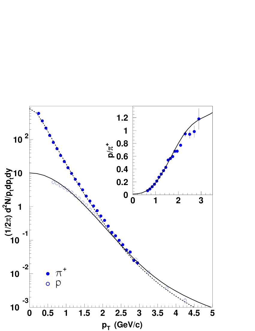
Figure 1: (Color online) Invariant $\pi^{+}$ and $p$ distributions as a function of $p_{t}$ for $T=117$ MeV, $R=8$ fm and $\beta_{\pi}=0.6$ and $\beta_{p}=0.53$. Also shown in the insert is the ratio $p/\pi^{+}$ of these distributions. Data are from Ref. PHENIXBM for collisions with $0-10\%$ of centrality.

Summing over all the states, the invariant thermal distribution for bosons and fermions are given by

$$E\frac{d^{3}N_{\mbox{\small{b}}}}{d^{3}p} = {\mathcal{N}}_{\mbox{\small{b}}}\sum_{nl}\frac{(2l+1)}{(2\pi)}\frac{k_{nl}^{2}E_{nl}\ e^{-\bar{\gamma}E_{nl}/T}}{\sqrt{p^{2}+\left(\frac{\bar{\gamma}\beta k_{nl}}{2RT}\right)^{2}}}$$ (11)

$$\times \frac{\left|J_{l+1/2}\left(pR-i\frac{\bar{\gamma}\beta k_{nl}}{2T}\right)\right|^{2}}{\left[p^{2}-k_{nl}^{2}-\left(\frac{\bar{\gamma}\beta k_{nl}}{2RT}\right)^{2}\right]^{2}+\left[\frac{\bar{\gamma}\beta pk_{nl}}{RT}\right]^{2}},$$

$$E\frac{d^{3}N_{\mbox{\small{f}}}}{d^{3}p} = {\mathcal{N}}_{\mbox{\small{f}}}\sum_{nl}\frac{(2l+1)}{(2\pi)}$$ (12)

$$\times \left[\frac{(E_{nl}^{2}+m^{2}+p^{2})+(\beta k_{nl}/2RT)^{2}}{m^{2}}\right]$$

$$\times \frac{k_{nl}^{2}E_{nl}\ e^{-\bar{\gamma}E_{nl}/T}}{\sqrt{p^{2}+\left(\frac{\bar{\gamma}\beta k_{nl}}{2RT}\right)^{2}}}$$

$$\times \frac{\left|J_{l+1/2}\left(pR-i\frac{\bar{\gamma}\beta k_{nl}}{2T}\right)\right|^{2}}{\left[p^{2}-k_{nl}^{2}-\left(\frac{\bar{\gamma}\beta k_{nl}}{2RT}\right)^{2}\right]^{2}+\left[\frac{\bar{\gamma}\beta pk_{nl}}{RT}\right]^{2}},$$

respectively. The factor $(2l+1)$ in Eqs. (11) and (12) comes from the degeneracy of a state with a given angular momentum eigenvalue $l$. ${\mathcal{N}}_{\mbox{\small{b}}}$ and ${\mathcal{N}}_{\mbox{\small{f}}}$ are normalization constants.

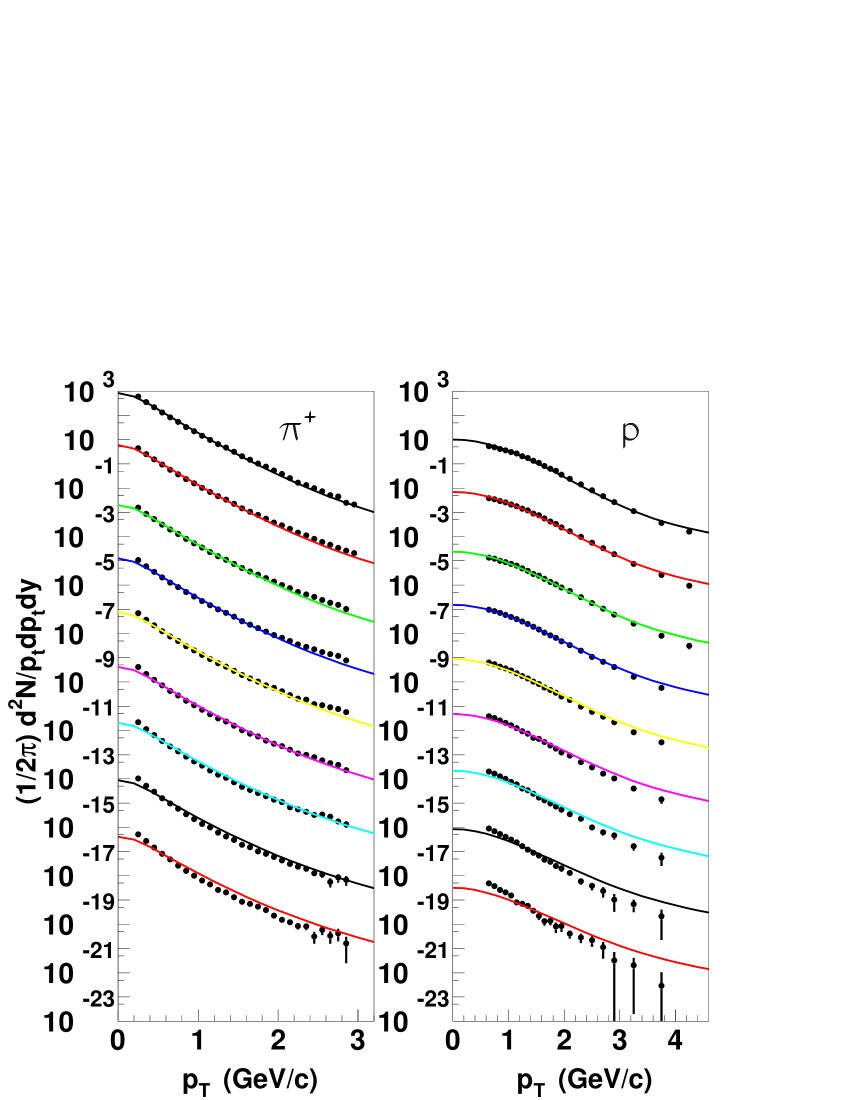
Figure 2: (Color online) Invariant $\pi^{+}$ (left panel) and $p$ (right panel) distributions as a function of $p_{t}$ for different collision centralities. The uppermost curves correspond to the most central collisions, $0-10\%$ with the centrality decreasing in intervals of $10\%$ PHENIXBM multiplied by successive factors of $10^{-2}$. The size of the equivalent spherical region is calculated according to the relation $R=R_{0}+C(N_{\mbox{\tiny{part}}}/2)^{1/3}$, with $R_{0}=1$ fm and $C=1.28$. The curves represent the theoretical calculation with $T_{\mbox{\small{$p,\pi$}}}=117$ MeV, $\beta_{\mbox{\small{$\pi$}}}=0.6$ and $\beta_{\mbox{\small{$p$}}}=0.53$, which describe the most central collisions data.

The contrast between a calculation with and without finite size effects, can be appreciated by looking at Fig. 5 in Ref. Ayalanew were it is shown a comparison between the invariant pion distribution as a function of $p_{t}$ computed for $T=120$ MeV, $\beta=0.6$ with finite size effects ($R=8$ fm) and without them. The curves are also compared to data on positive pions from PHENIX PHENIXBM . We notice from the figure that the curve with finite size effects does a very good job describing the data for all values of $p_{t}$ in this range. In contrast, a calculation where no effects of a finite size are included, and thus the wave function of a given state is simply a plane wave, does not describe the data over the considered range when use is made of the same values for $T$ and $\beta$ as for the case of the calculation with a confining volume.

III Transverse spectra

We now compare the model to data on mid-rapidity positive pions together with protons from central Au + Au collisions at $\sqrt{s_{NN}}=200$ GeV measured in RHIC PHENIXBM . We perform a $\chi^{2}$ fit to each spectra. The fit parameters are the pion and proton fireball radii, $R_{\mbox{\small{$\pi$}}}$, $R_{\mbox{\small{$p$}}}$, temperatures $T_{\mbox{\small{$\pi$}}}$, $T_{\mbox{\small{$p$}}}$, surface radial flow velocities $\beta_{\mbox{\small{$\pi$}}}$, $\beta_{\mbox{\small{$p$}}}$ and normalizations ${\mathcal{N}}_{\mbox{\small{$\pi$}}}$, ${\mathcal{N}}_{\mbox{\small{$p$}}}$. Based on the success of the description of the central rapidity pion data obtained in Ref. Ayalanew up to $p_{t}\sim 3$ GeV, we first fix the parameters describing the pion data with the minimization procedure. The parameters thus obtained are $R_{\mbox{\small{$\pi$}}}=8$ fm, $T_{\mbox{\small{$\pi$}}}=117$ MeV and $\beta_{\mbox{\small{$\pi$}}}=0.6$ which are basically the same as the ones obtained in Ref. Ayalanew were only the normalization was left as a free parameter and the rest were set to reasonable values that describe freeze-out conditions at RHIC.

Next, in order to find the parameters that describe the proton spectrum, we fix the values of any two of the parameters $R_{\mbox{\small{$p$}}}$, $T_{\mbox{\small{$p$}}}$ and $\beta_{\mbox{\small{$p$}}}$ to be the same as the corresponding parameters describing the pions, leaving the third parameter, along with the normalization constant ${\mathcal{N}}_{\mbox{\small{$p$}}}$ free. The optimum set of parameters obtained with this procedure correspond to $R_{\mbox{\small{$p$}}}=8$ fm, $T_{\mbox{\small{$p$}}}=117$ MeV and $\beta_{\mbox{\small{$p$}}}=0.53$. Figure 1 shows the distributions for pions and protons for central collisions $(0-10\%)$ PHENIXBM compared to the theoretical calculation with the best parameters obtained. We notice that the proton data are well described by the model up to $p_{t}\sim 3$ GeV for a temperature and system’s size equal to the corresponding parameters for the pions but that the magnitude of $\beta_{\mbox{\small{$p$}}}$ is about 10% smaller than $\beta_{\mbox{\small{$\pi$}}}$. We recall that in order to find an analytical expression for the momentum distributions, we resorted to approximate the gamma factor in Eq. (9) by the average gamma factor in Eq. (10). Since the effect of the same radial flow is stronger for particles with larger mass, it is therefore natural to expect that with this approximation we introduce a discrepancy in the description of the flow for particles with different masses. Nevertheless, we feel that an error of order 10% is acceptable considering the advantage of working with analytical expressions.

centrality	$N_{\mbox{\tiny{part}}}$	$R$ (fm)
$0-10\%$	325.2	8.0
$10-20\%$	234.6	7.3
$20-30\%$	166.6	6.6
$30-40\%$	114.2	5.9
$40-50\%$	74.4	5.3
$50-60\%$	45.5	4.6
$60-70\%$	25.7	4.0
$70-80\%$	13.4	3.4
$80-92\%$	6.3	2.9

Table 1: Parameters $N_{\mbox{\tiny{part}}}$ and $R$ for the description of the pion and proton spectra corresponding to different centralities. The radii of the equivalent spherical region has been calculated according to the relation $R=R_{0}+C(N_{\mbox{\tiny{part}}}/2)^{1/3}$, with $R_{0}=1$ fm and $C=1.28$.

We also notice that the description of the proton data for $p_{t}>3$ GeV is not as good. This can be understood recalling that for large $p_{t}$ the leading particle production mechanism is the fragmentation of fast moving partons, some of which fragment outside the fireball region and thus are not influenced by the confining boundary that the rest of the particles experience within the fireball and thus, that our description is not valid for these large $p_{t}$ particles.

Figure 2 shows the distributions for pions and protons for different collision centralities. For the description of these data, we have fixed the values of $T_{\mbox{\small{$p,\pi$}}}$ and $\beta_{\mbox{\small{$p,\pi$}}}$ to the ones obtained from the most central collisions analysis leaving the normalizations to be determined by the minimization procedure. The size of the overlap region for peripheral collisions has been determined from the number of participants $N_{\mbox{\tiny{part}}}$ in the reaction PHENIXBM by a simple scaling law for the size of the equivalent spherical region according to the relation $R=R_{0}+C(N_{\mbox{\tiny{part}}}/2)^{1/3}$, with $R_{0}=1$ fm and $C=1.28$ that gives $R=8$ fm for the most central region $(0-10\%)$ data. This relation is motivated by the similar one that gives the radius of a nucleus in terms of the mass number. The value of $R_{0}$ tries to account for the finite size of the interaction region as the number of participants takes its smallest value for the most peripheral collision, namely, $N_{\mbox{\tiny{part}}}=2$.

The values for $R$ and $N_{\mbox{\tiny{part}}}$ are listed on Table 1. We notice that the pion data are well described for all centralities except at the lower end of the spectra where a thermal calculation is expected to fail due to resonance contamination. The proton data is well described up to $p_{t}\sim 3$ GeV only up to centralities of order $40-50\%$ from where the quality of the description decreases as the centrality of the collisions decreases. We interpret the poor description of the proton data for $p_{t}>3$ GeV for all centralities as an indication that the leading particle production is not a kind of thermal parton recombination but instead the fragmentation of fast moving partons. On the other hand, the failure to describe proton data for centralities smaller that $40-50\%$ could be attributed to a different scaling of the effective size of the interaction region with $N_{\mbox{\tiny{part}}}$ as compared to the one obeyed by the pions or to the fact that for large impact parameters, the proton size becomes comparable to the size of the interaction region. An analysis to explore these possibilities will be presented elsewhere.

IV Particle Correlations

In order to explore the space-time dimensions of the system created in high-energy heavy-ion collisions, one typically looks at two-particle correlation functions. In the present case, it is thus instructive to look at this function to see whether the size scale that can be extracted from a two-particle correlation is comparable to the intrinsic scale dimension used in the model formulation. We carry out the analysis for the two-pion correlation function. For the purposes of this section, we closely follow Ref. Zhang to where we refer the reader for details.

Let $\psi_{nlm^{\prime}}({\mathbf{p}})$ represent the Fourier transform of the wave function for the state with quantum numbers $n,l.m^{\prime}$, namely

$$\psi_{nlm^{\prime}}({\mathbf{p}})=\int\frac{d^{3}r}{(2\pi)^{3}}e^{-i{\mathbf{p}\cdot\mathbf{r}}}\psi_{nlm^{\prime}}({\mathbf{r}})\,.$$ (13)

With the normalization adopted in Eq. (2), the one-pion momentum distribution can be represented as

$$P_{1}({\mathbf{p}}) \equiv \frac{d^{3}N}{d^{3}p}$$ (14)

$$= \sum_{n,l,m^{\prime}}2E_{nl}e^{-\bar{\gamma}E_{nl}/T}\psi_{nlm^{\prime}}^{*}({\mathbf{p}})\psi_{nlm^{\prime}}({\mathbf{p}})\,.$$

Similarly, and under the assumption of a complete factorization of the two-particle density matrix, the two pion momentum distribution can be written as

$$P_{2}({\mathbf{p}_{1}},{\mathbf{p}_{2}}) \equiv \frac{d^{6}N}{d^{3}p_{1}d^{3}p_{2}}$$

$$= P_{1}({\mathbf{p}_{1}})P_{1}({\mathbf{p}_{2}})$$

$$+ \left|\sum_{nlm^{\prime}}2E_{nl}e^{-\bar{\gamma}E_{nl}/T}\psi_{nlm^{\prime}}^{*}({\mathbf{p}_{1}})\psi_{nlm^{\prime}}({\mathbf{p}_{2}})\right|^{2},$$

from where the two-pion correlation function $C_{2}$ can be written, in terms of $P_{1}$ and $P_{2}$, as

$$C_{2}({\mathbf{p}_{1}},{\mathbf{p}_{2}})\! = \!\frac{P_{2}({\mathbf{p}_{1}},{\mathbf{p}_{2}})}{P_{1}({\mathbf{p}_{1}})P_{1}({\mathbf{p}_{2}})}.$$ (16)

Notice that as a consequence of the factorization assumption, the correlation function is such that $C_{2}({\mathbf{p}},{\mathbf{p}})=2$.

For the spherically symmetric problem here described, the correlation function depends on the magnitude, as well as on the angle between the momenta of the two particles ${\bf p}_{1}$ and ${\bf p}_{2}$. We make the change of variables to relative ${\bf q}={\bf p}_{1}-{\bf p}_{2}$ and average ${\bf K}=({\bf p}_{1}+{\bf p}_{2})/2$ momenta and also to the angle between these last two vectors, $\theta$. The correlation function thus becomes a function of $K=|{\bf K}|$, $q=|{\bf q}|$ and $\theta$. In order to consider the contribution from pions with different angles between their momenta, we average over $\theta$. Figure 3 shows $C_{2}(q)$ averaged over $\theta$ and for a fixed value $K=260$ MeV as a function of $q$ for $R=8$ fm, $T=117$ MeV and $\beta=0.55$. The solid curve shows the corresponding Gaussian fit.

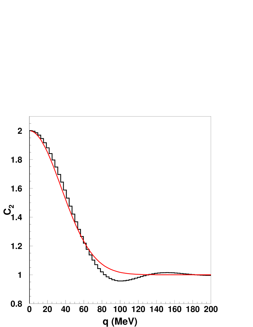
Figure 3: (Color online) $C_{2}(q)$ averaged over the angle between ${\bf K}$ and ${\bf q}$ as a function of $q$ for $K=260$ MeV, $R=8$ fm, $T=117$ MeV and $\beta=0.55$. The histogram corresponds to the model calculation whereas the solid curve shows the corresponding Gaussian fit.

In order to extract the system’s size $R_{\mbox{\tiny{eff}}}$ from this function, we fit this curve to a Gaussian distribution of the form

$$g(q) = 1+\rho^{2}(q),$$

$$\rho(q) = \exp(-q^{2}R_{\mbox{\tiny{eff}}}^{2}/2).$$ (17)

Figure 4 shows the behavior of $R_{\mbox{\tiny{eff}}}$ as a function of $(N_{\mbox{\tiny{part}}})^{1/3}$ compared to measured values for $R_{\mbox{\tiny{side}}}$ PHENIXcorr from Au + Au collisions at $\sqrt{s_{NN}}=200$ GeV. The lower solid curve corresponds to our model effective radii whereas the upper solid curve is the model curve displaced by a constant $\tilde{R}=0.8$ fm. The dashed curve corresponds to the best linear fit to the data. We notice that the slope of our model curve is in good agreement with the data. The fact that the intercept is different from zero may indicate the existence of correlation scales in the data that are not considered in our simple approach.

Finally, recall that

$$\rho(r)=\exp(-r^{2}/2R_{\mbox{\tiny{eff}}}^{2})$$ (18)

is the spherically symmetric three-dimensional distribution in space that gives rise to $\rho(q)$ upon Fourier transformation and that the $R_{r.m.s.}$ radius from $\rho(r)$ is given by

$$R_{r.m.s.}=\sqrt{3}R_{\mbox{\tiny{eff}}}.$$ (19)

On the other hand, for a rigid sphere, such as the distribution giving rise to our model distribution, the $R_{r.m.s.}$ radius is given by

$$R_{r.m.s.}=\sqrt{3/5}R.$$ (20)

By equating these two r.m.s. radii, we see that in order to compare the effective radius with the model one, the relation between them is given by

$$R=\sqrt{5}R_{\mbox{\tiny{eff}}}.$$ (21)

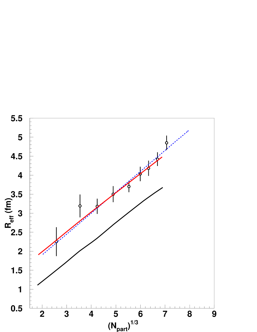
Figure 4: (Color online) $R_{\mbox{\tiny{eff}}}$ as a function of $(N_{\mbox{\tiny{part}}})^{1/3}$ for $K=260$ MeV compared to measured values for $R_{\mbox{\tiny{side}}}$ from Au + Au collisions at $\sqrt{s_{NN}}=200$ GeV. The lower solid curve corresponds to the model effective radii whereas the upper solid curve is the model curve displaced by a constant $R_{0}=0.8$ fm. The dashed curve is the best linear fit to the data

V Conclusions

In conclusion, we have shown that by considering the finite size of the interaction region and a simple scaling law of this with the number of participants in the collision, it is possible to achieve a good description of mid-rapidity pion and proton data in Au + Au collisions at RHIC with common values of temperature and transverse expansion velocity. For central collisions, the proton to pion ratio is also well described and its behavior can be attributed to the strength of the radial flow achieved in RHIC. By performing a two-particle correlation analysis and comparing to data for $R_{\mbox{\tiny{side}}}$ as a function of $(N_{\mbox{\tiny{part}}})^{1/3}$ from Au + Au collisions at $\sqrt{s_{NN}}=200$ GeV, we see that the scaling law found from the single particle spectra analysis is in good agreement provided that we displace our model curve by a constant $\tilde{R}=0.8$ fm and we speculate that this signals the existence of an extra correlation length in data that is not accounted for in our simple model.

We should stress that the spherical symmetry assumed throughout can be thought of as a theoretical tool rather than as a realistic approximation to the actual collision geometry for the highest RHIC energies. Our intention is to provide a working model with a high degree of symmetry that can be better controlled in an actual calculation. The same is true for the treatment of the shape of the region for non-central collisions which one knows, from elliptic flow analyses, that partially retains the original almond shape of the overlap region in the collision. The sizes referred to in this way reflect characteristic sizes rather than actual spherical radii. Although modifying the geometry used for the calculation will certainly give rise to a different set of quantum states, the bulk of the effect will remain since the physics that it captures is the Heisenberg uncertainty principle whereby restricting the size of the region to become finite, the momentum states become broader. As for the use of stationary states, we point out that although the freeze-out volume is reached with a large expansion velocity, the transition from a strongly interacting system to a free gas is rapid and what matters is the distribution right before this transition and therefore the length scale associated to it.

It is important to emphasize that a description of the transverse distributions for different impact parameters can be done by considering a varying freeze-out temperature and radial velocity but the lesson to be learned from the present analysis is that this variation can be tempered and/or even avoided by considering the finite size of the interaction region.

We point out that some hydrodynamical models without finite size effects have been able to give similarly good descriptions of data up to $p_{t}$ of order 2-2.5 GeV Schnedermann at the expense of introducing a large amount of parameters. What we have shown here is that it is also possible to achieve the same quality of description including a basic property of quantum systems often neglected, that is the fact that in high energy reactions, particles are produced in small space-time regions. While doing this and in this first step approach, we made use of approximations to render the calculations tractable, one of such is the treatment of the gamma Lorentz factor in terms of an average one. The relaxation of these approximations is a natural step forward and we will report on the progress of this work elsewhere.

The authors thank G. Paic for his valuable comments and suggestions. Support for this work has been received by PAPIIT-UNAM under grant number IN107105 and CONACyT under grant numbers 40025-F and bilateral agreement CONACyT-CNPq J200.556/2004 and 491227/2004-3.

References

- (1) S.S. Adler et al. (PHENIX Collaboration), Phys. Rev. C 69, 034909 (2004).
- (2) R. C. Hwa and C. B. Yang, Phys. Rev. C 67, 034902 (2003); R. J. Fries, B. Müller, C. Nonaka, and S. A. Bass, Phys. Rev. Lett. 90, 202303 (2003); V. Greco, C. M. Ko, and P. Lévai, Phys. Rev. Lett. 90, 202302 (2003).
- (3) I. Tserruya, Pramana 60, 577 (2003).
- (4) J. Adams et al., (STAR Collaboration), nucl-ex/0601033.
- (5) C.M. Hung and E. Shuryak, Phys. Rev. C 57, 1891 (1998).
- (6) A. Ayala, J. Bareiro and L.M. Montaño, Phys. Rev. C60, 014904 (1999).
- (7) J. Adams et al. (STAR Collaboration), Nucl. Phys. A 757, 102 (2005).
- (8) K.H. Ackermann, (STAR Collaboration), Phys. Rev. Lett 86, 402 (2001)
- (9) D. Adamová et al., (CERES Collaboration), Phys. Rev. Lett. 90, 022301 (2003).
- (10) E.S. Fraga and R. Venugopalan, Braz. J. Phys. 34, 315 (2004); Physica A 345, 121 (2004).
- (11) F. Becattini, J. Phys. Conf. Ser. 5, 175 (2005).
- (12) Q.H. Zhang and S.S. Padula, Phys. Rev. C 62, 024902 (2000); Q.H. Zhang, hep-ph/0106242.
- (13) A. Ayala and A. Sánchez, Phys. Rev. C 63, 064901 (2001).
- (14) E.V. Shuryak, Phys. Rev. D42, 1764 (1990).
- (15) A. Ayala, E. Cuautle, J. Magnin, L.M. Montaño and A. Raya, Phys. Lett. B 634, 200 (2006).
- (16) A. Ayala and A. Smerzi, Phys. Lett. B 405, 20 (1997).
- (17) S. Adler et al. (PHENIX Collaboration), Phys. Rev. Lett. 93, 152302 (2004).
- (18) E. Schnedermann, J. Sollfrank and U. Heinz, Phys. Rev. C 48, 2462 (1993).