From non-Hermitian effective operators to large-scale no-core shell model calculations for light nuclei

Abstract

No-core shell model (NCSM) calculations using ab initio effective interactions are very successful in reproducing experimental nuclear spectra. The main theoretical approach is the use of effective operators, which include correlations left out by the truncation of the model space to a numerically tractable size. We review recent applications of the effective operator approach, within a NCSM framework, to the renormalization of the nucleon-nucleon interaction, as well as scalar and tensor operators.

1 Introduction

The theory of effective operators plays an important role in the modern approach to nuclear structure. Effective interactions are the basic ingredient of the no-core shell model (NCSM), one of the ab initio methods that provides solution to the nuclear many-body problem starting from high precision nucleon-nucleon (NN) interactions (i.e., that describe the two-nucleon data with high accuracy) and theoretical three-nucleon forces.

Numerical solution to the $A$–body Schrödinger equation can be obtained only if one truncates the Hilbert space to a finite, yet sufficiently small dimension. Restriction of the space to a numerically tractable size requires that operators for physical observables be replaced by effective operators that are designed to account for such effects. Most applications of the effective operator theory are limited to deriving effective interactions, but other observables are of great interest as well. In particular, for electromagnetic operators, a long standing problem in the phenomenological shell model was the use of effective charges for protons and neutrons. Perturbation theory has been partially successful in describing empirical effective charges needed to explain experimental transition strengths [1]. However, recent investigations using the unitary transformation approach within the framework of the NCSM to obtain effective operators have reported some progress in explaining the large values of the empirical effective charges [2]. We will discuss briefly this result and its consequences later.

In the restricted space, the effective operators are constructed to reproduce the values of the corresponding physical observables in the full space. However, the renormalization procedure usually alters properties of bare operators; for example, the interaction is no longer Hermitian, and general transition operators change their rotational symmetry properties. While in some cases non-Hermitian Hamiltonians have advantages [3], in our case this presents a major inconvenience. Moreover, some approaches introduce energy dependence of the resulting effective operators, an additional complication for solving the nuclear many-body problem. This drawback is, however, avoided in the unitary transformation approach to effective operators of Okubo [4] and others [5, 6, 7, 8]. This method allows us to construct all effective operators in an energy independent form, and, through an additional similarity transformation, to restore the Hermiticity of the effective interaction and the roattional properties of transition operators.

This paper is organized as follows: we review the theoretical approach in Sec. 2, and then apply the procedure in realistic cases, using realistic two-body interactions, for the Hamiltonian in Sec. 3, and other general operators in Sec. 4. We draw our conclusions in Sec. 5.

2 Theoretical Approach

In this section we review the similarity transformation approach to effective operators and discuss its practical implementation in the case of the nuclear many-body Hamiltonian.

2.1 Formal theory

It is not our intention to discuss in great detail the method; we will point out the main features, following the derivation in Refs. [9] and [10].

In our approach, the full Hilbert space is divided into a model space, with associated projection operator $P$, and a complementary, excluded space, with the associated projection operator $Q$ ($P+Q=1$). The goal is to perform many-body calculations in the model space, using a transformed Hamiltonian $\mathcal{H}$,

$${\mathcal{H}}=XHX^{-1},$$ (1)

so that a finite subset of eigenvalues of the initial Hamiltonian $H$ are reproduced. We need to point out that this is a general approach, which can be applied to non-Hermitian Hamiltonian operators that can arise, for example, in the context of boson mappings.

To better understand the conditions that we will impose on the transformation operator $X$, we start with the results of the Feshbach projection formalism on the Schrödinger equation

$${\mathcal{H}}|\Psi\rangle=E_{\Psi}|\Psi\rangle.$$ (2)

In general for non-Hermitian Hamiltonians, the left and right eigenvectors are not related simply by a Hermitian conjugation, but we have the freedom to choose a normalization so that $\langle\tilde{\Psi}_{E}|\Psi_{E}\rangle=1$, where $\langle\tilde{\Psi}_{E}|$ is the left eigenvector corresponding to the eigenvalue $E_{\Psi}$. It follows from Eq. (2) that the component of the wave function $|\Psi\rangle$ outside the model space is given by

$$Q|\Psi\rangle=\frac{1}{E_{\Psi}-Q{\mathcal{H}}Q}Q{\mathcal{H}}P|\Psi\rangle,$$ (3)

so that the effective Hamiltonian in the model space can be expressed as

$$H_{eff}=P{\mathcal{H}}P+P{\mathcal{H}}Q\frac{1}{E-Q{\mathcal{H}}Q}Q{\mathcal{H}}P.$$ (4)

An immediate consequence of Eq. (4) is that in order to obtain an energy independent Hamiltonian in the model space, it is sufficient to impose one of the following decoupling conditions

$$Q{\mathcal{H}}P=0,$$ (5)

or

$$P{\mathcal{H}}Q=0$$ (6)

We note, however, that the former condition also ensures that the $Q$-space component of the wave function $|\Psi\rangle$ vanishes, although this is not true for its complementary left eigenstate. Moreover, as it will become clear in the derivation of the effective operators below, both conditions have to be satisfied so that one obtains energy-independent effective operators corresponding to other observables besides the Hamiltonian.

In the case of general operators, $O$, properly transformed by the same transformation operator $X$, e.g., the Hamiltonian $H$ in Eq. (1), one has to compute a matrix element of the form $\langle\tilde{\Phi}|{\mathcal{O}}|\Psi\rangle$, where $\langle\tilde{\Phi}|$ corresponds possibly to another left eigenvector of ${\mathcal{H}}$. Using the fact that the $Q$-component of the left eigenstate $\langle\tilde{\Phi}|$ can be written similarly to Eq. (3)

$$\langle\tilde{\Phi}|Q=\langle\tilde{\Phi}|P{\mathcal{H}}Q\frac{1}{E_{\Phi}-Q{\mathcal{H}}Q},$$ (7)

one can extract the expression for the effective operator in the model space $P$

$${\mathcal{O}}_{eff}=P{\mathcal{O}}P+P{\mathcal{H}}Q\frac{1}{E_{\Phi}-Q{\mathcal{H}}Q}Q{\mathcal{O}}P+P{\mathcal{O}}Q\frac{1}{E_{\Psi}-Q{\mathcal{H}}Q}Q{\cal H}P$$ (8)

$$+P{\mathcal{H}}Q\frac{1}{E_{\Phi}-Q{\mathcal{H}}Q}Q{\mathcal{O}}Q\frac{1}{E_{\Psi}-Q{\mathcal{H}}Q}Q{\cal H}P.$$

As advertised, in order to obtain an energy-independent expression for a general effective operator one needs to construct the transformation operator $X$ so that both decoupling conditions (5) and (6) are satisfied. Consequently, both left and right $P$ eigenstates of the transformed Hamiltonian ${\mathcal{H}}$ have components only in the model space. A number of other subtleties exist within this effective operator approach [11].

In order to determine the transformation $X$, we consider the following ansatz [9, 10]

$$X=\exp(-\omega)\exp(\Omega),$$ (9)

with the new operators fulfilling the additional requrements

$$\omega=Q\omega P,$$

$$\Omega=P\Omega Q.$$

Hence, the decoupling condition (5) transforms into a quadratic equation for $\omega$

$$Q{\mathcal{H}}P=QHP-Q\omega HP+QH\omega P-\omega H\omega=0,$$ (10)

which does not depend on $\Omega$, while the decoupling condition (6) becomes a linear equation for $\Omega$

$$P{\mathcal{H}}Q=PHQ+P\Omega HQ-Q\Omega\omega HQ-PH\Omega Q-PH\omega\Omega Q=0.$$ (11)

The result of applying such a transformation is the following expressions for the effective Hamiltonian

$${\mathcal{H}}_{eff}=PHP+PH\omega,$$ (12)

which is manifestly non-Hermitian, even if the original Hamiltonian $H$ is Hermitian, and for general effective operators:

$${\mathcal{O}}_{eff}=(P+\Omega-\Omega\omega)O(P+\omega),$$ (13)

which also changes symmetry properties under the Hermitian conjugation operation.

We have made no assumption up to now about the original Hamiltonian, but in most cases of interest, $H$ is Hermitian. For such applications, one can introduce an additional transformation [12], so that the effective Hamiltonian in the model space is also Hermitian [9]

$${\mathcal{H}}_{eff}=\frac{P+\omega^{\dagger}}{\sqrt{P+\omega^{\dagger}\omega}}H\frac{P+\omega}{\sqrt{P+\omega^{\dagger}\omega}}.$$ (14)

Moreover, for Hermitian Hamiltonians one finds $\Omega=(P+\omega^{\dagger}\omega)^{-1}\omega^{\dagger}$ [9], so that a general effective operator can also be written similarly to the effective Hamiltonian, i.e., involving only the operator $\omega$

$${\mathcal{O}}_{eff}=\frac{P+\omega^{\dagger}}{\sqrt{P+\omega^{\dagger}\omega}}O\frac{P+\omega}{\sqrt{P+\omega^{\dagger}\omega}}.$$ (15)

There are two iterative solutions of Eq. (10) that determine the transformation operator $\omega$: one that converges to the states with the largest $P$-space components and is equivalent to the solution of Krenciglowa and Kuo [13], and another which converges to states lying closest to a chosen parameter appearing in the iteration procedure [6, 7]. However, we present here a more efficient method to find $\omega$. It relies on the fact that the components of the exact eigenvectors in the complementary space are mapped into the model space. Thus, a simple and efficient means to compute the matrix elements of $\omega$ is [14]

$$\langle\alpha_{Q}|\omega|\alpha_{P}\rangle=\sum_{k\in{\mathcal{K}}}\langle\alpha_{Q}|\Psi_{k}\rangle\langle{\Psi_{k}}|\alpha_{P}\rangle^{-1},$$ (16)

where $|\alpha_{P}\rangle$ and $|\alpha_{Q}\rangle$ are the basis states of the $P$ and $Q$ spaces, respectively, and $|\Psi_{k}\rangle$ denotes states from a selected set ${\mathcal{K}}$ of exact eigenvectors of the Hamiltonian in the full space. The dimension of the subspace ${\mathcal{K}}$ is equal with the dimension of the model space $P$. In the next subsection, we will present a practical implementation of Eq. (16).

To conclude this brief review of the formal effective operator theory, we would like to reiterate the main idea: in order to obtain energy-independent operators in a restricted model space, it is sufficient to design a transformation $X$ so that all the matrix elements of the transformed Hamiltonian connecting the model and the excluded space are identically zero, i.e., Eqs. (5) and (6) are simultaneously satisfied. Making the ansatz in Eq. (9), one can find equations which determine the transformation, so that the decoupling conditions are satisfied. Finally, in the case of Hermitian Hamiltonians, such as the many-body nuclear Hamiltonain, we gave the general expressions for the effective Hamiltonian and effective operators in the model space. Even in this case, one can, in principle, obtain non-Hermitian effective Hamiltonains, but one can always make an additional transformation to obtain a Hermitian structure, which is much more convenient to apply to the description of a system of $A$ nucleons using realistic interactions.

2.2 Application to the nuclear Hamiltonian

We assume that the system of $A$ nucleons is described by the non-relativistic intrinsic Hamiltonian

$$H_{A}=\frac{1}{A}\sum_{i<j=1}^{A}\frac{p_{ij}^{2}}{2m}+\sum_{i<j=1}^{A}V_{ij}^{NN},$$

where $\vec{p}_{ij}=\vec{p}_{i}-\vec{p}_{j}$ are the relative momenta between two nucleons, and $V_{ij}^{NN}$ the NN potential, such as the local Argonne $v_{18}$ [15, 16] or the non-local charge dependent Bonn potential [17], which describe with high accuracy the experimental two-nucleon data. The generalization to include three-body forces is straightforward, but much more involved (see, e.g., Ref. [18]). Thus, for the purpose of this paper, we neglect three-body forces.

In the NCSM approach, the single-particle wave functions are described using harmonic oscillator (HO) states. One then constructs many-body states using a restricted set of one-body HO states. The model space is determined by the requirement that the the many-body basis states can have up to $N_{max}\hbar\Omega$ excitations above the minimum energy configuration, where $\hbar\Omega$ is the HO energy parameter and $N_{max}$ is an integer. Including all states up to a given HO energy allows us to separate exactly by projection containing spurious center-of-mass (CM) motion, even when we work in a non-translationally invariant basis.

As seen explicitly in Eq. (16), the solution of the $A$-body problem is required in order to solve for the transformation operator $\omega$. However, the eigenvectors $|\Psi_{k}\rangle$ are, in principle, the final goal, as they allow computation of any properties of the system. To practically implement the method to solve many-body problems, we introduce the cluster approximation. This consists in finding $\omega$ for the $a$-body problem, $a<A$, and then using the effective interaction thus obtained for solving the $A$-body system. There are two limiting cases of the cluster approximation: first, when $a\rightarrow A$, the solution becomes exact; a higher-order cluster is a better approximation and was shown to increase the rate of convergence [18, 19]. Second, when $P\rightarrow 1$, the effective interaction approaches the bare interaction; as a result, the cluster approximation effects can be minimized by increasing as much as possible the size of the model-space size.

We emphasize that in the $a$-body cluster approximation the explicit decoupling conditions in Eqs. (5)–(6) are now fulfilled only for the $a$-body problem:

$$Q_{a}{\mathcal{H}}^{(a)}P_{a}=Q_{a}X_{a}{H}_{a}X_{a}^{-1}P_{a}=0,$$

where $P_{a}$, $Q_{a}$ refer to the corresponding projection operators for the $a$-particle system. Conditions (5)–(6) are, in general, violated for the $A$-body problem, but the errors become smaller with increasing the size of the model space.

The rate of convergence for a fixed cluster approximation can be improved by adding to $H_{A}$ a CM Hamiltonian, which also provides a single-particle HO basis for performing numerical calculations. Doing this, we obtain

$$H_{A}^{\Omega}=H_{A}+\frac{\vec{P}^{2}}{2mA}+\frac{1}{2}mA\Omega^{2}R^{2}$$ (17)

$$=\sum_{i=1}^{A}\left[\frac{\vec{p}_{i}^{2}}{2m}+\frac{1}{2}m\Omega^{2}\vec{r}_{i}^{2}\right]+\sum_{i>j=1}^{A}\left[V_{ij}^{NN}-\frac{m\Omega^{2}}{2A}(\vec{r}_{i}-\vec{r}_{j})^{2}\right]$$

$$=\sum_{i=1}^{A}h_{i}+\sum_{i>j=1}^{A}v_{ij}\;,$$

In a $a$-body cluster approximation, this ensures a dependence of the transformation, and, therefore, of the effective interaction on $A$. The CM term does not introduce any net influence on the converged intrinsic properties of the many-body calculation, as we subtract it in the final many-body calculation. Moreover, although this addition and subtraction does not affect our exact treatment of the CM motion, this procedure introduces a pseudo-dependence upon the HO energy $\hbar\Omega$, and the two-body cluster approximation described above will exhibit this dependence. In the largest model spaces, however, important observables manifest a considerable independence of the energy $\hbar\Omega$ and the model space size, i.e., the value of $N_{max}$.

Finally, note that even if the original Hamiltonian contained just one- and two-body terms, the operator $X$, the transformed Hamiltonian ${\mathcal{H}}_{eff}$ [by means of Eq. (14)] and transformed operators [by means of Eq. (15)] all contain up to irreducible $a$-body terms. (The exact effective operators contain up to irreducible $A$-body terms.)

3 Application to effective interactions

The first application of the effective operator theory in the context of the NCSM is to compute an effective interaction in a restricted model space. While the cluster approximation described in Sec. 2 is general for $a$ nucleons, we are currently limited by the complexity of the calculations to $a\leq 3$.

In Figure 1 we present the results for ⁴He, using both the two- and three-body cluster approximations. In the left panel, we show both the ground- and excited-state energies using HO energies of 19 and 28 MeV and a three-body cluster in order to compute the effective interaction for ⁴He, starting from the CD Bonn interaction [17]. The convergence pattern shows a dependence upon the HO energy. Thus, the ground-state energy converges faster when $\hbar\Omega=28$ MeV, but both HO energies eventually converge to the exact result obtained by solving, e.g., the Fadeev-Yakubovski equations [20]. The complete convergence of the ground-state energy can be obtained within the NCSM, as demonstrated, e.g., in Fig. 1 of Ref. [21]. Because we neglect three-body interactions, the converged result misses by a few MeV the experimental value. Unlike for the ground state, the first $0^{+}$ excited-state energy has a faster convergence rate for $\hbar\Omega=19$ MeV. However, this state converges much more slowly than the ground state, and even in the largest model spaces the results are quite sensitive to the choice of the HO energy parameter.

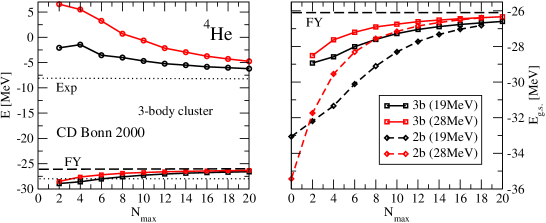
Figure 1: ⁴He: dependence of the ground- and excited-state energies on $N_{max}$ in the three-body cluster approximation (left panel), and comparison of the convergence rates of the ground-state energy for the two- and three-body cluster approximations (right panel). Two different HO energies (19 and 28 MeV) have been used in each case. The dashed line is the exact ground-state energy [20] for the CD Bonn potential used in this investigation, while the dotted lines represent the experimental ground- and first excited-state energies.

As expected, a higher-body cluster approximation includes more correlations in the interactions, and the convergence is faster. This is illustrated in the right panel of Fig. 1, where we plot the ground-state energy dependence on $N_{max}$ obtained by computing the effective interaction using both the two- and three-body cluster approximations. The rate of convergence is faster in the three-body cluster approximation for both HO energies chosen for this example.

We have used ⁴He in this section to illustrate the convergence properties of effective interactions, but the method has been applied successfully to the description of the spectra of $p$ shell nuclei [14, 18, 22, 23, 24] and beyond.

4 Application to general operators

So far, most applications of the NCSM approach have been to calculating the effective interaction, and only a few of publications [2, 25, 26, 27] have investigated the renormalization of general operators in realistic calculations of nuclear properties. In Ref. [2] Navrátil et al. performed large-basis NCSM calculations, which were later explicitly truncated into a $0\hbar\Omega$ space and fitted to one-body quadrupole operators. By construction these calculations contained all correlations up to six-body due to the truncation and, hence, yielded the large effective charge renormalizations of $1.5\;e$ for protons and $0.5\;e$ for neutrons found empirically. However, the full space renormalization of selected electromagnetic operators has been reported only relatively recently [26, 27]. We review below the results for one- and two-body operators.

4.1 One-body operators

In the $a$-body cluster approximation, the effective operators corresponding to an one-body operator will have, in general, irreducible $a$-body terms. The simplest approximation is the two-body cluster. In order to apply it, one has to rewrite the original one-body contributions as a sum of two-body terms. For details on this procedure, we refer the reader to, e.g., Refs. [25, 26].

In the case of the quadrupole operator, we follow the procedure described in Ref. [26]. Selected $B(E2)$ results, obtained using the two-body cluster approximation for ⁶Li and ^12,14C are presented in Table 1. We have performed calculations with effective operators only in small model spaces for several reasons. First, as expected from the convergence properties of effective operators mentioned in Sec. 2, larger renormalization effects are expected in smaller model spaces. Second, the application of the procedure for tensor operators is much more involved, since they can connect states with different angular momentum or/and isospin. Hence, in Eq. (15) one can have different transformation operators $\omega$ to the left and to the right of the bare operator. Moreover, the number of two-body matrix elements for non-scalar operators can be orders of magnitude larger than the number of one-body matrix elements. Finally, the main purpose of these investigations was a qualitative understanding of the influence of effective operators and not a highly accurate description of the experimental data.

Table 1: $B(E2)$, in $e^{2}fm^{4}$, for selected nuclei and model spaces, using the bare operator and the effective operator, computed in the two-body cluster approximation.

• Nucleus	Observable	Model Space	Bare operator	Effective operator
  6Li	$B(E2,1^{+}0\rightarrow 3^{+}0)$	0$2\hbar\Omega$	02.647	2.784
  6Li	$B(E2,1^{+}0\rightarrow 3^{+}0)$	$10\hbar\Omega$	10.221	–
  6Li	$B(E2,2^{+}0\rightarrow 1^{+}0)$	0$2\hbar\Omega$	02.183	2.269
  6Li	$B(E2,2^{+}0\rightarrow 1^{+}0)$	$10\hbar\Omega$	04.502	–
  10C	$B(E2,2_{1}^{+}0\rightarrow 0^{+}0)$	0$4\hbar\Omega$	03.05	3.08
  12C	$B(E2,2_{1}^{+}0\rightarrow 0^{+}0)$	0$4\hbar\Omega$	04.03	4.05

As illustrated in Table 1, the effective operators have very little effect on the results for the qudrupole transitions. For ⁶Li, we also present the $B(E2)$ values obtained in $10\hbar\Omega$ model space [23]. If the effect of the renormalization of the quadrupole operator had been significant, then the $B(E2)$ values in the small model spaces would be closer to the results in the $10\hbar\Omega$ model space, which is obviously not the case. The same weak renormalization can be observed for the carbon isotopes, listed in Table 1. This is contrary to the previous investigation in the framework of the NCSM [2], which reported obtaining the correct effective proton and neutron phenomenological charges. However, the main difference is that the ⁶Li calculation in Ref. [2] included up to six-body correlations. Comparison of the two results suggests that higher-order clusters can play an important role in the renormalization of the quadrupole operator.

4.2 Two-body operators

In a previous publication [26], we used a two-body Gaussian operator to demonstrate the dependence of the renormalization upon the range of the operator. In a recent paper [27], we computed the longitudinal-longitudinal distribution function, part of the inclusive $(e,e^{\prime})$ response. In this paper we present similar results, obtained in smaller model spaces but converged nevertheless at high momentum transfer (=short range), because we use the appropriate effective operators. Moreover, the effect of the renormalization is larger in smaller model spaces, as noted before.

To define the longitudinal-longitudinal distribution function, one starts with the Coulomb sum rule

$$S_{L}(q)=\frac{1}{Z}\int_{\omega_{el}}^{\infty}d\omega S_{L}(q,\omega),$$ (18)

which is the total integrated strength measured in electron scattering. In Eq. (18), $S_{L}(q,\omega)=R(q,\omega)/|G_{E,p}(q,\omega)|^{2}$, with $R(q,\omega)$ the longitudinal response function and $G_{E,p}(q,\omega)$ the proton electric form factor, while $\omega_{el}$ is the energy of the recoiling $A$-nucleon system with $Z$ protons. $S_{L}(q),$ which is related to the Fourier transform of the proton-proton distribution function [28, 29], can be expressed in terms of the longitudinal form factor $F_{L}(q)$ and the longitudinal-longitudinal distribution function $\rho_{LL}$ as [30]

$$S_{L}(q) = \frac{1}{Z}\langle g.s.|\rho_{L}^{\dagger}(\mathbf{q})\rho_{L}(\mathbf{q})|g.s.\rangle-\frac{1}{Z}|\langle g.s.|\rho_{L}(\mathbf{q})|g.s.\rangle|^{2}$$

$$\equiv 1+\rho_{LL}(q)-ZF_{L}(q)/G_{E,p}(q,\omega_{el}).$$

If one neglects relativistic corrections and two-body currents, then $\rho_{L}(\mathbf{q})$ is the charge operator,

$$\rho_{L}(\mathbf{q})=\frac{1}{2}\sum_{i=1}^{A}\exp(i\mathbf{q}\cdot\mathbf{r}_{i})(1+\tau_{z,i}),$$

so that the longitudinal-longitudinal distribution function becomes [30]

$$\rho_{LL}(q)=\frac{1}{4Z}\sum_{i\neq j}\langle g.s.|j_{0}(q|\mathbf{r}_{i}-\mathbf{r}_{j}|)(1+\tau_{z,i})(1+\tau_{z,j})|g.s.\rangle.$$

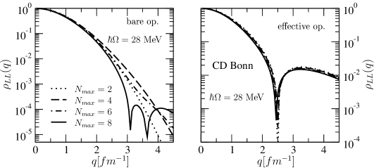
Figure 2: The longitudinal-longitudinal distribution function in ⁴He, obtained using bare operators (left panel) and effective operators (right panel). The HO energy used in this calculation was $\hbar\Omega=28$ MeV, while the NN interaction was CD Bonn.

In Figure 2 we present the results for the longitudinal-longitudinal distribution function for ⁴He. At high momentum transfer, the results obtained using bare operators depend strongly upon the model space. On the other hand, the results obtained with effective operators are model space invariant at high $q$, although Figure 1 shows that the wave function is not fully converged, since the energy is not converged in these very small model spaces. They agree with the values computed in larger model spaces and different HO energies given in Ref. [27]. At intermediate momentum transfer, i.e., $q\approx 2.5$ fm^-1, even the effective operator results vary. This effect is due to the fact that the long range part of the operator has not yet converged in these small model spaces.

Similar results for the longitudinal-longitudinal distribution function have been obtained for ¹²C, where calculations in very large model spaces are not possible. However, even in the smallest model space, $0\hbar\Omega$, we were able to obtain good results for high momentum transfer, which reproduce the values in larger model spaces [27].

As demonstrated in Ref. [26] with a two-body Gaussian operator and illustrated here for the longitudinal-longitudinal distribution function, in the two-body cluster approximation the renormalization depends strongly of the range of the operator. Short range operators (high momentum transfer) are very well renormalized and the results become model-space independent even in the two-body cluster approximation, while long-range operators, such as the quadrupole transition operator, or the longitudinal-longitudinal distribution function for small and intermediate momentum transfer, are only weakly renormalized.

5 Conclusions

In this paper, we have reviewed the application of the effective operator theory in the framework of the NCSM. While in the derivation one can obtain non-Hermitian operators that are more suitable for some applications [3], we construct, by means of additional transformations, Hermitian operators, which are easier to utilize in large scale calculations.

The ab initio NCSM has been applied successfully to the description of the nuclear spectra for light nuclei [14, 18, 22, 23, 24], i.e., $A\leq 16$, and beyond [31, 32]. The wave functions obtained can be used to calculate and predict nuclear properties, such as the proton radii of halo nuclei [33], or the astrophysical $S$-factor [34], to cite just a couple of the most recent results. Moreover, for light nuclei, the precision of the NCSM method makes it possible to investigate the reliability of the chiral nuclear interaction. This follows from the fact that the properties, e.g., energy spectra, of $p$-shell nuclei are sensitive to the subleading parts of the chiral interactions, including three-nucleon forces [35]. For heavier nuclei, another approach, designed to improve the convergence of the results, has been recently proposed, combining the inverse $J$-matrix scattering technique and the NCSM [36].

In the two-body cluster approximation, one has now the ability to compute not only the effective interaction, but also the consistent effective operators corresponding to scalar and tensor observables. We have shown a strong dependence on the renormalization of the range of the bare operator. Thus, if the operator is of short range, then one obtains a good renormalization in the two-body cluster approximation, as the unitary transformation used to obtain the effective interaction renormalizes mostly the short-range repulsion of the potential. Consequently, one obtains model-space independence results for such observables. Long-range operators, on the other hand, are only weakly renormalized at the two-body cluster level. In order to accomodate the long-range correlations one has to increase the model space and/or use a higher-order cluster approximation. The success of latter was demonstrated by the good results for the $0\hbar\Omega$ effective charges obtained in a restricted NCSM calculation [2].

References

- [1] Ellis P J and Osnes E 1974 Rev. Mod. Phys. 49 777
- [2] Navrátil P, Thoresen M and Barrett B R 1997 Phys. Rev. C 55 573
- [3] Bender C M, Chen J-H and Milton K A 2006 J. Phys. A 39 1657
- [4] Okubo S 1954 Prog. Theor. Phys. 12 603
- [5] Da Providencia J and Shakin C M 1964 Ann. of Phys. 30 95
- [6] Suzuki K and Lee S Y 1980 Prog. Theor. Phys. 64 2091
- [7] Suzuki K 1992 Prog. Theor. Phys. 68 1999
- [8] Suzuki K and Okamoto R 1994 Prog. Theor. Phys. 92 1045
- [9] Navrátil P, Geyer H B and Kuo T T S 1993 Phys. Lett. B 315 1
- [10] Navrátil P and Geyer H B 1993 Nucl. Phys. A 556 165
- [11] Viazminsky C P and Vary J P 2001 J. Math. Phys. 42 2055
- [12] Scholtz F G, Geyer H B and Hahne F J W 1992 Ann. Phys. (NY) 23 74
- [13] Krenciglowa E M and Kuo T T S 1974 Nucl. Phys. A 235 171
- [14] Navrátil P, Vary J P and Barrett B R 2000 Phys. Rev. C 62 054311
- [15] Wiringa R B, Stocks V G J and R. Schiavilla 1995 Phys. Rev. C 51 38
- [16] Pieper S and Wiringa R B 2001 Annu. Rev. Nucl. Part. Sci. 51 53
- [17] Machleidt R, Sammarruca F and Song Y 1996 Phys. Rev. C 53 1483
- [18] Navrátil P and Ormand W E 2003 Phys. Rev. C 68 034305
- [19] Navrátil P and Ormand W E 2003 Phys. Rev. Lett. 88 152502
- [20] Nogga A private communication
- [21] Navrátil P, Ormand W E, Forssén C and Caurier E 2005 Eur. Phys. J. 25 481
- [22] Navrátil P, Vary J P and Barrett B R. 2000 Phys. Rev. Lett. 84 5728
- [23] Navrátil P, Vary J P, Ormand W E and Barrett B R 2001 Phys. Rev. Lett. 87 172502
- [24] Forssén C, Navrátil P, Ormand W E and Caurier E 2005 Phys. Rev. C 71 044312
- [25] Stetcu I, Barrett B R, Navrátil P and Johnson C W 2004 Int. J. Mod. Phys. E 14 95
- [26] Stetcu I, Barrett B R, Navrátil P and Vary J P 2005 Phys. Rev. C 71 044325
- [27] Stetcu I, Barrett B R, Navrátil P and Vary J P 2006 Phys. Rev. C in press (Preprint nucl-th/0601076)
- [28] Drell S D and Schwartz C L 1958 Phys. Rev. 122 568
- [29] McVoy K W and Van Hove L 1962 Phys. Rev. 125 1034
- [30] Schiavilla R, Wiringa R B and Carlson J 1993 Phys. Rev. Lett. 70 3856
- [31] See, e.g., 20Ne example in P. Navrátil’s talk http://www.int.washington.edu/talks/WorkShops/int_05_3/
- [32] Vary J P et. al. 2005 Eur. Phys. J. A 25 475
- [33] Caurier E and Navrátil P 2006 Phys. Rev. C 73 021302(R)
- [34] Navrátil P, Bertulani C A and Caurier E 2006 Phys. Lett. B 634 191
- [35] Nogga A, Navrátil P, Barrett B R and Vary J P 2005 Preprint nucl-th/0511082
- [36] Shirokov A M, Vary J P, Mazur A I and Weber T A 2005 Phys. Lett. B 621 96