Relativistic interactions for the meson-two-nucleon system in the clothed-particle unitary representation

Abstract

The method of unitary clothing transformations put forward in relativistic quantum field theory (QFT) by Greenberg and Schweber and developed by Shirokov is applied to construct a new family of interactions in the meson-two-nucleon system. Along with a brief exposition of its basic elements we show a specific transition from the initial “bare” one-meson and one-nucleon operators and states to their physical “clothed” counterparts. We emphasize that the clothing transformations in question do not alter the original total Hamiltonian, but provides a conceptually more transparent representation of the same Hamiltonian in terms of a new set of operators for particles with physical properties and their relativistic interactions. The Hermitian and energy-independent interaction operators for the processes $\pi N\rightarrow\pi N$, $NN\rightarrow NN$ and $NN\leftrightarrow\pi NN$ are derived starting from the Yukawa-type couplings between fermions (nucleons and antinucleons) and bosons ($\pi-$, $\eta-$, $\rho-$, $\omega-$ mesons, etc.). These types of interaction have a distinctive off-energy-shell structure which is naturally generated by the unitary transformation that removes from the Hamiltonian the (three-leg) $\pi$NN vertex coupling.

I Introduction

To view the light hadronic systems as few-body systems involves several problematic aspects, and many of these aspects still need to be theoretically explored in detail. Not all cases are so fortunate that one can accurately reduce the underlying field-theoretical problem to a non-relativistic quantum-mechanical Hamiltonian formulation in a (two-body, three-body, etc.) potential scheme. One fortunate situation occurs typically in low-energy few-nucleon physics Aren , where the considered degrees of freedom are the nucleons, and the non-relativistic interactions are generated via meson-exchange processes, or via alternative, effective field-theoretical derivations. But, even in this well-defined research area, there have been attempts to brake the paradigm of the purely nucleonic Hamiltonian description in the potential scheme Canetal , and to relate the origin of well-known unsolved problems, such as the $A_{y}$ puzzle, to dynamical effects of the pion CanScha .

As the energy increases, the light hadronic systems become much more problematic to be described. The opening of the pionic threshold forces to deal directly with the pion degrees of freedom. This complicates the few-body equations since one has to deal simultaneously with phenomena of production and absorption of particles garzila-mizuta . The derivation of non-perturbative dynamical equations for meson-few-nucleon processes is still waiting for a consistent theory that solves the general problem in a feasible and calculable way.

Specific topics, such as the study of $NN\rightarrow NN\pi$ inelasticities, both in free space and in more complex nuclear environments, have received much attention recently. Many phenomenological works have attempted the description of the experimental data, including polarization data, and extensive reviews on the past and current status of research on this subject are availablegarzila-mizuta ; haiden ; hanardt ; Dubna1995 ; Cracow1996 . In general, such models perform some nonrelativistic reduction of the interaction Hamiltonian between mesons and nucleons, and construct the basic production mechanisms using perturbative schemes. Typically, these terms consist of the $\pi$NN one-body term (direct term plus recoil) and some more complex two-nucleon processes such as pion rescattering, intermediate $\Delta$ excitations, and 2N processes involving heavy-meson exchange currents. As yet, there is not a clear-cut understanding of which mechanisms contribute the most and, especially in the isoscalar channel at threshold (the channel of the pp$\rightarrow$pp$\pi^{o}$ process) there has been quite a debate on which are the basic mechanisms that provide the strength to the threshold cross section. This strength can be generated either by short-range heavy-meson exchanges lee-riska , or by pion rescatterings in the $\sigma$ channel hernandez-oset . Presently, the analysis of the $NN\rightarrow NN\pi$ inelasticities did not succeed to resolve this ambiguity, and there is hope that the study of more complex reactions, such as $pd\rightarrow\pi^{o}\ He^{3}$, can help to solve this ambiguity. Phenomenological studies for this reaction have been limited to calculations involving only pion rescattering in the $\sigma$-channel Canton-Schadow ; these calculations achieved, very recently, a good reproduction of data for both angular distributions for the excitation function and for the analyzing power Canton-Levchuk . For this 3N reaction, a thorough study involving production mechanisms originated also by 2N heavy-meson exchanges is needed, but unfortunately these studies have still to come.

Besides the problem of constructing the 2N heavy-meson exchange mechanisms in a consistent manner (we will come back to this problem in the final part of this paper), there remain, in addition, several difficulties that need to be explored. One is related to the need to use relativistic equations for the nucleon dynamics in the energy range of meson production, since this energy range is higher than the typical low-energy nuclear regime where nonrelativistic quantum mechanics works so well. Then, the first step is to construct consistent relativistic (pseudo) potentials that fulfill the Poincaré algebra.

Another difficulty is connected with the treatment of virtual effects generated by the $\pi$NN vertex in the production process. To directly use the one-body vertex and similar operators in the construction of one-body-type production mechanisms may create serious difficulties because in the $\pi NN$ vertex the three particles cannot stay simultaneously on-mass-shell. However, the use of quantum-mechanical equations for the nucleon dynamics forces the nucleons on their mass shell, and the pion, being the physical observed particle in the production process, has also to stay on its mass shell. Clearly, all this creates ambiguities in the possible treatment of one-body operators, and hence there are problems of internal inconsistencies in the construction and calculation of sets of one-body, two-body, etc, operators. This represents a not negligible problem in pion production at threshold: although the magnitude of the one-body term is generally small, the interference effects of the one-body term with respect to the more dominant two-body amplitudes have important consequences in the cross sections.

A similar difficulty also occurs when the elementary fermion-meson vertex interaction is used for the construction of meson decays operators in relativistic constituent quark models. It has been shown recently that the use of the spectator-model ansatz (built upon the elementary quark-meson vertex) in Relativistic Quantum Mechanics (RQM) is not fully constrained in covariant calculations of strong (meson) decays of baryon resonances. This aspect has been pointed out in Ref. MelCanPleWag specifically for the construction of spectator-model operators in the so-called Point-Form formulation of RQM. However, the presence of ambiguities in the general construction of Current Operators has been observed in all forms of RQM, including front form and instant form Lev95 .

The approach illustrated in this paper represents a field-theoretic way to overcome the above mentioned difficulties. Among the varieties of field-theoretical approaches we concentrate on the Unitary-Transformation (UT) methods for Hamiltonian-based models. UT’s do not change the expressions for the observables, because the $S$-matrix remains the same under such transformations. However, the unitary transformations allow to change the representation of the Hamiltonian so that the interaction operators refers to particles with physical (observable) properties. It is important that the interactions extracted this way are Hermitian, energy-independent and include the off-shell structures naturally. These attractive features of the unitary transformation approaches allow to derive pion-production interaction operators that are relativistic and involve only physical particles (and hence, one-body operators are eliminated from the representation and all the virtual processes or effects are embedded in the interaction operators); we also extend the calculation to include 2N heavy-meson exchange mechanisms for the production amplitude, given the importance that these mechanisms have in discussing the phenomenology of 3N forces and pion production.

There have been quite different implementations of UT techniques (see Ref. SheShi2001 and refs. therein, for a review). In such approaches one starts with the original field Hamiltonian $H$, to arrive at a new representation of $H$ which is unitarily equivalent and where the particles involved interact through interaction operators that are energy independent. Such energy independence simplifies the solution of the eigenvalue problem for the initial Hamiltonian. To avoid the confusion that already exists in the literature, we do not employ here the inflated term “effective” to qualify our interactions, since they have no direct connections (that we are aware of) with the formalisms of effective Lagrangians.

Amongst the different UT formalisms, we mention first Okubo’s idea Okubo.Progr.Theor.Phys.12.603.1954 to block-diagonalize $H$ via a UT with respect to the decomposition of the full Fock space $\mathcal{R}_{F}$ of hadronic states into the nucleon (no-meson) subspace and its complement in $\mathcal{R}_{F}$. The Okubo approach was further developed by Glöckle and Müller GlockleMuller.Phys.Rev.C23.1183.1981 in their relativistic theory of interacting particles. These authors were the first to show, al least to our knowledge, how with the help of one single UT the non-commuting Hermitian operators (Hamiltonian and Lorentz boosts) can be reduced to a block form. For a simple model of ”spinless nucleons” exchanging scalar mesons, it was then possible to construct the new Hermitian and energy independent contributions to the Poincaré group generators.

In Ref. KorchinShebekoPhysAtNucl1993 the same method was employed for deriving the nucleon-nucleon and nucleon-antinucleon interactions starting from a field Hamiltonian with the exchange of $\pi-$, $\rho-$, $\omega-$ and $\sigma-$ mesons. Then, in the framework of the Hartree approximation, these interactions have been introduced to describe the saturation properties of nuclear matter. That approximation, we note in passing, gives rise to an original recipe (see Eqs. (23)-(25) in KorchinShebekoPhysAtNucl1993 ) for calculating the nucleon mass shift in the three dimensional approach.

Fuda and co-workers Fuda.Ann.Phys.231.1.1994 , FudaZhang.Phys.Rev.C51.23.1995 , FudaZhang.Phys.Rev.C54.495.1996 , ElmessiriFuda.Phys.Rev.C60.044001.1999 have also used the Okubo-Glöckle-Müller approach to construct one-boson-exchange models in light-front dynamics. They prefer to work with the mass-square operator $M^{2}$ rather than with $H$ because the former commutes with all of the Poincaré generators. Such studies demonstrated that the two-particle interactions obtained in second-order perturbation theory have certain similarities but do not coincide exactly with the relevant Born terms obtained using the Feynman-diagram techniques (see also Ref. KorchinShebekoPhysAtNucl1993 ). We shall address this question in more detail in Sec. 3.

Successful applications of the UT method have been obtained also in the theory of nuclear forces and nuclear electromagnetic processes (see Refs. SatoTamuraNiwaOhtsuboJ.Phys.G.17.303.1991 , KobayashiSatoOhtsuboProgrTheorPhys1997 with reference to earlier studies of the 50’s, e.g., Ref. Nishijima1956 ). Such developments by the Osaka group KobayashiSatoOhtsuboProgrTheorPhys1997 illustrate another useful application of the UT formalism: the elimination from $H$ of certain virtual processes whose $S$-matrix elements, by definition, have to vanish on the energy shell. Remarkably, the transformed Hamiltonian $H^{\prime}=U^{\dagger}HU$ contains only interactions for real processes. Even more remarkably, it was possible to derive the one-pion-exchange (OPE) and two-pion-exchange (TPE) nucleon-nucleon potentials, the pion-nucleon potential (see also SatoLee.Phys.Rev.C54.2660.1996 ), the $N\Delta\rightarrow NN$ transition potential, the interactions for pion absorption/production, and so on, from one and the same initial Hamiltonian $H$ without any additional ad hoc assumption (of physical or mathematical nature) in each case. The corresponding Hermitian energy-independent operators are defined in the complete $\mathcal{R}_{F}$, i.e., not only in a subspace $\subset\mathcal{R}_{F}$ as was the case for Okubo approach.

In the present work, we construct the meson-baryon interaction operators relying upon the notion of ”clothed” particles. Such notion was introduced many years ago by Greenberg and Schweber GRESCH58 (see also Chapter XII in the monograph SchweberBook ) in their aim to include the so-called cloud or persistent effects (the terminology refers back to Van Hove vanHove.Physica.21.901.1955 , vanHove.Physica.22.343.1956 ). In this connection, we apply the method of unitary clothing transformations elaborated by FaddeevDokl.AkadNauk.USSR.1963.152.573 and ShirokovVisinescuRevRoumPhys1974 and developed recently in Refs. SheShi97 , SheShi98 , SheShi2000 , SheShi2001 . In this way, a large amount of virtual processes induced by the meson absorption/emission, the $N\bar{N}$ -pair annihilation/production and other cloud effects can be accumulated in the creation (destruction) operators for the clothed (physical) mesons and nucleons. Such a bootstrap reflects the most significant distinction between the concepts of clothed and bare particles.

The approach used in this article differs from the aforementioned ones at least in two aspects. First, the clothing procedure does not aim, a priori, to define a UT that blockdiagonalizes $H$, as is done in the Okubo approach. Besides, it might be not always possible to implement such a task in the infinite-dimensional Hilbert space. Instead, the aim of the multistep clothing procedure is to express the original Hamiltonian $H$ in terms of the new clothed-particle operators in a form which is different than that given for the initial bare-particle ones. Such a transition from the bare-particle representation (BPR) to the clothed-particle representation (CPR) introduces a new sparse structure of the original Hamiltonian $H$. Second, in the framework of the CPR the mass and vertex renormalization problem SheShi2001 , KordaShebekoPhys.Rev.2004 is considered in a natural way, in parallel with the construction of the interactions, while the renormalization problem in Ref. KobayashiSatoOhtsuboProgrTheorPhys1997 has been disregarded. Other distinctions are discussed in Sects. 2 and 3.

In this context, we would like to draw attention to the recent work by Stefanovich on the problem of divergences in QFT. As was shown in Ref. StefanovichAnnPhys2001 , one can introduce a similarity transformation $U^{\dagger}HU$ to cancel infinite counterterms directly in $H$ and therefore also in the $S$-matrix operator. As an application, the method has been illustrated for the case of an Hamiltonian system in quantum electrodynamics. Although Ref. StefanovichAnnPhys2001 does not use the clothing ideas, there are many points of contact between that approach and the CPR method and, in our opinion, further developments in this area could have promising perspectives.

The central goal of this paper is the derivation of interaction operators in the CPR for the processes $\pi N\rightarrow\pi N$, $NN\rightarrow NN$ and $NN\leftrightarrow\pi NN$. For the field-theoretical treatment of mesons and nucleons we assume the instant form after Dirac of relativistic dynamics, in which the generators of space translations and rotations are the same as in the free theory. We remind that in this case the three boost operators must involve the interaction parts to meet, together with the total Hamiltonian $H$, the well-known commutation relations of the Poincaré-Lie algebra. At the beginning we prefer to consider $H$ as a function of creation and destruction operators in the Fock space rather than the more customary form that follows from a given field Lagrangian. Our option follows a general statement that $H$ may be expressed as a sum of products of creation and destruction operators (see Chapter III of Ref. WeinbergBook1995 ). This Hamilton formulation of RQFT simplifies the introduction of the CPR that we consider in this work.

The outline of this paper is as follows. The aspects of the method of unitary clothing transformations, which are necessary for constructing a new family of interactions operators in the meson-two-nucleon system are illustrated in Sec. 2. We introduce an auxiliary UT’s that convert the primary bare bosons and fermions into some intermediate-level particles with physical masses. The approach develops along the chain: bare particles with bare masses $\to$ bare particles with physical masses $\to$ physical (observable) particles. This procedure is useful for drawing some parallels between the clothing approach in QFT and the method of canonical transformations (in particular, the Bogoliubov ones) in the theory of superfluidity and superconductivity. Analytical expressions for the relativistic interactions (quasipotentials) in the CPR are shown in Sec. 3 in case of the primary Yukawa coupling between pions and nucleons. Our calculations are performed using purely algebraic means within an iterative technique proposed in that Section. The features that distinguish the obtained momentum-space quasipotentials from their on-energy-shell counterparts derived in the second-order Dyson perturbation theory with Feynman rules are emphasized. Explicit formulae for the quasipotentials generated by the additional heavier-meson exchange mechanisms are given in Sec. 4.

II Formalism

II.1 Introductory definitions

Our departure point is the Hamiltonian

$$H=H(\stackrel{{\scriptstyle\circ}}{{\alpha}})=H_{0}(\stackrel{{\scriptstyle\circ}}{{\alpha}})+V_{0}(\stackrel{{\scriptstyle\circ}}{{\alpha}}),$$ (1)

where the unperturbed Hamiltonian $H_{0}(\stackrel{{\scriptstyle\circ}}{{\alpha}})$ and the interaction term $V_{0}(\stackrel{{\scriptstyle\circ}}{{\alpha}})$ depend on the creation and destruction operators of the “bare” particles with unphysical masses and coupling constants. Here, $\stackrel{{\scriptstyle\circ}}{{\alpha}}$ denotes the set of all these operators. For example, in case of a spinor (fermion) field $\psi$ and a neutral pseudoscalar meson field $\phi$ one has to introduce the operators $\stackrel{{\scriptstyle\circ}}{{a}}\left(\mathbf{k}\right)$, $\stackrel{{\scriptstyle\circ}}{{b}}\left(\mathbf{p},r\right)$, $\stackrel{{\scriptstyle\circ}}{{d}}\left(\mathbf{p},r\right)$ and their adjoint counterparts, respectively, for mesons, nucleons and antinucleons. These operators enter in the expansions

$$\phi\left(\mathbf{x}\right)=\left(2\pi\right)^{-3/2}\int d\mathbf{k}\left(2\omega_{\mathbf{k}}^{\circ}\right)^{-1/2}\left[\stackrel{{\scriptstyle\circ}}{{a}}(\mathbf{k})+\stackrel{{\scriptstyle\circ}}{{a}}{}^{\dagger}(-\mathbf{k})\right]\exp(i\mathbf{kx}),$$ (2)

$$\pi\left(\mathbf{x}\right)=-i\left(2\pi\right)^{-3/2}\int d\mathbf{k}\left(\omega_{\mathbf{k}}^{\circ}/2\right)^{1/2}\left[\stackrel{{\scriptstyle\circ}}{{a}}(\mathbf{k})-\stackrel{{\scriptstyle\circ}}{{a}}{}^{\dagger}(-\mathbf{k})\right]\exp(i\mathbf{kx}),$$ (3)

$$\psi\left(\mathbf{x}\right)=\left(2\pi\right)^{-3/2}\int d\mathbf{p}\left(m_{0}/E_{\mathbf{p}}^{\circ}\right)^{1/2}\sum_{r,i}\stackrel{{\scriptstyle\circ}}{{U}}_{i}\left(\mathbf{p},r\right)\stackrel{{\scriptstyle\circ}}{{F}}_{i}\left(\mathbf{p},r\right)\exp(i\mathbf{px}).$$ (4)

In the last expression we have introduced the following matrix notations

$$\stackrel{{\scriptstyle\circ}}{{U}}\left(\mathbf{p},r\right)=\left(\begin{matrix}\stackrel{{\scriptstyle\circ}}{{U}}_{1}\left({\bf p},r\right)\cr\stackrel{{\scriptstyle\circ}}{{U}}_{2}\left({\bf p},r\right)\cr\end{matrix}\right)=\left(\begin{matrix}\stackrel{{\scriptstyle\circ}}{{u}}\left({\bf p},r\right)\cr\stackrel{{\scriptstyle\circ}}{{v}}\left(-{\bf p},r\right)\cr\end{matrix}\right),$$ (5)

$$\stackrel{{\scriptstyle\circ}}{{F}}\left(\mathbf{p},r\right)=\left(\begin{matrix}\stackrel{{\scriptstyle\circ}}{{F}}_{1}\left({\bf p},r\right)\cr\stackrel{{\scriptstyle\circ}}{{F}}_{2}\left({\bf p},r\right)\cr\end{matrix}\right)=\left(\begin{matrix}\stackrel{{\scriptstyle\circ}}{{b}}\left({\bf p},r\right)\cr\stackrel{{\scriptstyle\circ}}{{d}}{}^{\dagger}\left(-{\bf p},r\right)\cr\end{matrix}\right).$$ (6)

In other words, the lower index $i$ (the energy-sign index) in $\stackrel{{\scriptstyle\circ}}{{U_{i}}}\left(\mathbf{p},r\right)$and $\stackrel{{\scriptstyle\circ}}{{F_{i}}}\left(\mathbf{p},r\right)$reflects the particle-antiparticle degrees of freedom in the Dirac formalism. The quantities $\mathbf{k}$, $\mathbf{p}$ and $r$ are the particle momenta and the fermion polarization index. The two Dirac spinors $\stackrel{{\scriptstyle\circ}}{{u}}$ and $\stackrel{{\scriptstyle\circ}}{{v}}$ satisfy the conventional equations $(\not{p}^{\circ}-m_{0})~{}\stackrel{{\scriptstyle\circ}}{{u}}~{}\left(\mathbf{p},r\right)=~{}0$ and $(\not{p}^{\circ}+m_{0})\stackrel{{\scriptstyle\circ}}{{v}}\left(\mathbf{p},r\right)=0$ with $\not{p}^{\circ}=E_{\mathbf{p}}^{\circ}\gamma^{0}-\mathbf{p}\mbox{{${\bf\gamma}$} }$. The relativistic bare energies are expressed as $E_{\mathbf{p}}^{\circ}=\sqrt{\mathbf{p}^{2}+m_{0}^{2}}$ and $\omega_{\mathbf{k}}^{\circ}=\sqrt{\mathbf{k}^{2}+\mu_{0}^{2}}$, where the unknown values $m_{0}$ and $\mu_{0}$ play role of the bare (nonrenormalized) masses. As in Ref. SheShi2001 , we use throughout this paper the definition of the Dirac matrices, with orthonormalization as in Bjorken-Drell (Ref. BD64 ) for $\stackrel{{\scriptstyle\circ}}{{u}}$ and $\stackrel{{\scriptstyle\circ}}{{v}}$,

$$\stackrel{{\scriptstyle\circ}}{{U}}_{i}{}^{\dagger}\left(\mathbf{p},r\right)\stackrel{{\scriptstyle\circ}}{{U}}_{j}\left(\mathbf{p},r^{\prime}\right)=\frac{E_{\mathbf{p}}^{\circ}}{m_{0}}\delta_{i,j}\delta_{r,r^{\prime}}.$$ (7)

The operators $\stackrel{{\scriptstyle\circ}}{{a}}(\mathbf{k})$ and $\stackrel{{\scriptstyle\circ}}{{a}}{}^{\dagger}(\mathbf{k})$, $\stackrel{{\scriptstyle\circ}}{{b}}\left(\mathbf{p},r\right)$ and $\stackrel{{\scriptstyle\circ}}{{b}}^{\dagger}\left(\mathbf{p},r\right)$, $\stackrel{{\scriptstyle\circ}}{{d}}\left(\mathbf{p},r\right)$ and $\stackrel{{\scriptstyle\circ}}{{d}}^{\dagger}\left(\mathbf{p},r\right)$ satisfy the usual commutation relations

$$\left[\stackrel{{\scriptstyle\circ}}{{a}}\left(\mathbf{k}\right),\,\stackrel{{\scriptstyle\circ}}{{a}}^{\dagger}\left(\mathbf{k}^{\prime}\right)\right] = \delta(\mathbf{k}-\mathbf{k}^{\prime}),$$

$$\left\{\stackrel{{\scriptstyle\circ}}{{b}}\left(\mathbf{p},r\right),\stackrel{{\scriptstyle\circ}}{{b}}^{\dagger}\left(\mathbf{p}^{\prime},r^{\prime}\right)\right\} = \left\{\stackrel{{\scriptstyle\circ}}{{d}}\left(\mathbf{p},r\right),\stackrel{{\scriptstyle\circ}}{{d}}^{\dagger}\left(\mathbf{p}^{\prime},r^{\prime}\right)\right\}=\delta_{rr^{\prime}}\delta(\mathbf{p}-\mathbf{p}^{\prime}\mathbf{)}$$ (8)

which, in particular, yield

$$\left\{\stackrel{{\scriptstyle\circ}}{{F}}_{i}\left(\mathbf{p},r\right),\stackrel{{\scriptstyle\circ}}{{F}}_{j}{}^{\dagger}\left(\mathbf{p}^{\prime},r^{\prime}\right)\right\}=\delta_{i,j}\delta_{r,r^{\prime}}\delta(\mathbf{p}-\mathbf{p}^{\prime}).$$ (9)

In the BPR the corresponding unperturbed Hamiltonian is

$$H_{0}(\stackrel{{\scriptstyle\circ}}{{\alpha}})=\int d\mathbf{k}\omega_{\mathbf{k}}^{\circ}\stackrel{{\scriptstyle\circ}}{{a}}{}^{\dagger}\left(\mathbf{k}\right)\stackrel{{\scriptstyle\circ}}{{a}}\left(\mathbf{k}\right)+\int d\mathbf{p}E_{\mathbf{p}}^{\circ}\left[\stackrel{{\scriptstyle\circ}}{{b}}^{\dagger}\left(\mathbf{p},r\right)\stackrel{{\scriptstyle\circ}}{{b}}\left(\mathbf{p},r\right)+\stackrel{{\scriptstyle\circ}}{{d}}^{\dagger}\left(\mathbf{p},r\right)\stackrel{{\scriptstyle\circ}}{{d}}\left(\mathbf{p},r\right)\right].$$ (10)

By definition, the one-bare-fermion and one-bare-meson states $|\mathbf{p},r\rangle^{\circ}$ and $|\mathbf{k}\rangle^{\circ}$ are eigenstates of $H_{0}$ with eigenvalues ${E_{\mathbf{p}}^{\circ}}=\sqrt{\mathbf{p}^{2}+m_{0}^{2}}$ and $\omega_{\mathbf{k}}^{\circ}=\sqrt{\mathbf{k}^{2}+\mu_{0}^{2}}$. These states are built of the bare vacuum $\stackrel{{\scriptstyle\circ}}{{\Omega}}_{0}$, $|\mathbf{p},r\rangle^{\circ}=\stackrel{{\scriptstyle\circ}}{{b}}{}^{\dagger}(\mathbf{p},r)\ \stackrel{{\scriptstyle\circ}}{{\Omega}}_{0}$ and $|\mathbf{k}\rangle^{\circ}=\stackrel{{\scriptstyle\circ}}{{a}}{}^{\dagger}(\mathbf{k})\ \stackrel{{\scriptstyle\circ}}{{\Omega}}_{0}$, respectively. As usual, the no-bare-particle state $\stackrel{{\scriptstyle\circ}}{{\Omega}}_{0}$ is destroyed by the operators $\stackrel{{\scriptstyle\circ}}{{a}}$, $\stackrel{{\scriptstyle\circ}}{{b}}$ and $\stackrel{{\scriptstyle\circ}}{{d}}$, i. e., $\stackrel{{\scriptstyle\circ}}{{a}}(\mathbf{k})\stackrel{{\scriptstyle\circ}}{{\Omega}}_{0}=\stackrel{{\scriptstyle\circ}}{{b}}(\mathbf{p},r)\stackrel{{\scriptstyle\circ}}{{\Omega}}_{0}=\stackrel{{\scriptstyle\circ}}{{d}}(\mathbf{p},r)\stackrel{{\scriptstyle\circ}}{{\Omega}}_{0}=0$ for ${\forall\mathbf{k},\mathbf{p},r}$.

II.2 The mass-changing Bogoliubov-type unitary transformation

Now, let us consider a set $\alpha=(a,a^{\dagger},...)$ of destruction and creation operators for particles with generic masses $m$ and $\mu$. If $m$ and $\mu$ assume the physical values, the representation refers to “bare particles with physical masses” (see Ref. SheShi2001 ). By definition, the operators $\alpha$ enter in the following expansions of the same fields:

$$\phi\left(\mathbf{x}\right)=\left(2\pi\right)^{-3/2}\int d\mathbf{k}\left(2\omega_{\mathbf{k}}\right)^{-1/2}\left[a(\mathbf{k})+a^{\dagger}(-\mathbf{k})\right]\exp(i\mathbf{kx}),$$ (11)

$$\pi\left(\mathbf{x}\right)=-i\left(2\pi\right)^{-3/2}\int d\mathbf{k}\left(\omega_{\mathbf{k}}/2\right)^{1/2}\left[a(\mathbf{k})-a^{\dagger}(-\mathbf{k})\right]\exp(i\mathbf{kx}),$$ (12)

$$\psi\left(\mathbf{x}\right)\mathbf{=}\left(2\pi\right)^{-3/2}\int d\mathbf{p}\left(m/E_{\mathbf{p}}\right)^{1/2}\sum_{r,i}U_{i}\left(\mathbf{p},r\right)F_{i}\left(\mathbf{p},r\right)\exp(i\mathbf{px}),$$ (13)

where $u\left(\mathbf{p},r\right)$ and $v\left(\mathbf{p},r\right)$ are the Dirac spinors, which satisfy the equations

$$(\not{p}-~{}m)u\left(\mathbf{p},r\right) = 0$$

$$(\not{p}+m)v\left(\mathbf{p},r\right) = 0$$

with $\not{p}=E_{\mathbf{p}}\gamma^{0}-\mathbf{p}\mathbf{\gamma}$, $E_{\mathbf{p}}=\sqrt{\mathbf{p}^{2}+m^{2}}$ and $\omega_{\mathbf{k}}=\sqrt{\mathbf{k}^{2}+\mu^{2}}$. The spinor column $U\left(\mathbf{p},r\right)$ is composed of the spinors $u\left(\mathbf{p},r\right)$ and $v\left(-\mathbf{p},r\right)$ just as the column $\stackrel{{\scriptstyle\circ}}{{U}}\left(\mathbf{p},r\right)$ of $\stackrel{{\scriptstyle\circ}}{{u}}\left(\mathbf{p},r\right)$ and $\stackrel{{\scriptstyle\circ}}{{v}}\left(-\mathbf{p},r\right)$. Similarly, the operator column $F\left(\mathbf{p},r\right)$ is composed of the operators $b\left(\mathbf{p},r\right)$ and $d^{\dagger}\left(\mathbf{p},r\right)$ just as the column $\stackrel{{\scriptstyle\circ}}{{F}}\left(\mathbf{p},r\right)$ of $\stackrel{{\scriptstyle\circ}}{{b}}\left(\mathbf{p},r\right)$ and $\stackrel{{\scriptstyle\circ}}{{d}}^{\dagger}\left(\mathbf{p},r\right)$.

Comparing the expressions (11)-(13) and (2)-(4), we find the links

$$\frac{\stackrel{{\scriptstyle\circ}}{{a}}(\mathbf{k})+\stackrel{{\scriptstyle\circ}}{{a}}{}^{\dagger}(-\mathbf{k})}{\sqrt{\omega_{\mathbf{k}}^{\circ}}}=\frac{a(\mathbf{k})+a^{\dagger}(-\mathbf{k})}{\sqrt{\omega_{\mathbf{k}}}},\,{\forall\mathbf{k},}$$ (14)

$$\left(\stackrel{{\scriptstyle\circ}}{{a}}(\mathbf{k})-\stackrel{{\scriptstyle\circ}}{{a}}{}^{\dagger}(-\mathbf{k})\right)\sqrt{\omega_{\mathbf{k}}^{\circ}}=\left(a(\mathbf{k})-a^{\dagger}(-\mathbf{k})\right)\sqrt{\omega_{\mathbf{k}}},\,{\forall\mathbf{k},}$$ (15)

$$\sqrt{\frac{m_{0}}{E_{\mathbf{p}}^{\circ}}}\sum_{r,i}\stackrel{{\scriptstyle\circ}}{{U}}_{i}\left(\mathbf{p},r\right)\stackrel{{\scriptstyle\circ}}{{F}}_{i}\left(\mathbf{p},r\right)=\sqrt{\frac{m}{E_{\mathbf{p}}}}\sum_{r,i}U_{i}\left(\mathbf{p},r\right)F_{i}\left(\mathbf{p},r\right),\,{\forall\mathbf{p.}}$$ (16)

Moreover, operators $\alpha$ are assumed to meet the same commutation rules as operators $\stackrel{{\scriptstyle\circ}}{{\alpha}}$ do. Thus, the relations (9) are conserved as well. The orthogonality of $U\left(\mathbf{p}\right)$ follows from Eq. (7), after the substitution $m_{0}\rightarrow m$ ($E_{\mathbf{p}}^{\circ}\rightarrow E_{\mathbf{p}}$). Since the operators $\stackrel{{\scriptstyle\circ}}{{\alpha}}$ and $\alpha$ meet the same commutation relations, it is reasonable to look for a similarity (unitary) transformation

$$\stackrel{{\scriptstyle\circ}}{{a}}\left(\mathbf{k}\right)=Ta\left(\mathbf{k}\right)T^{\dagger},\,\,\stackrel{{\scriptstyle\circ}}{{b}}\left(\mathbf{p},r\right)=Tb\left(\mathbf{p},r\right)T^{\dagger},\,\,\stackrel{{\scriptstyle\circ}}{{d}}\left(\mathbf{p},r\right)=Td\left(\mathbf{p},r\right)T^{\dagger},$$ (17)

that connects them. We confine ourselves to the form $T=T_{mes}\otimes T_{ferm}$, where the UT’s $T_{mes}$ and $T_{ferm}$ act in mesonic and fermionic sectors respectively and generate the linear relations:

$$\stackrel{{\scriptstyle\circ}}{{a}}\left(\mathbf{k}\right)=T_{mes}a\left(\mathbf{k}\right)T_{mes}^{\dagger}=c_{1}(\mathbf{k})a(\mathbf{k})+c_{2}(\mathbf{k})a^{\dagger}(-\mathbf{k}),$$ (18)

with real functions $c_{1}(\mathbf{k})$ and $c_{2}(\mathbf{k})$ and

$$\stackrel{{\scriptstyle\circ}}{{F}}_{i}\left(\mathbf{p},r\right)=T_{ferm}F_{i}\left(\mathbf{p},r\right)T_{ferm}^{\dagger}=\sum_{j,r^{\prime}}O_{i,r;j,r^{\prime}}(\mathbf{p})F_{j}\left(\mathbf{p},r^{\prime}\right),$$ (19)

where for a given $\mathbf{p}$ the $c$-number coefficients $O_{i,r;j,r^{\prime}}(\mathbf{p})$ form a unitary 4$\times$4 matrix $O(\mathbf{p})$.

Evidently, the constraint $c_{1}^{2}-c_{2}^{2}=1$ is necessary to ensure the commutation $\left[a\left(\mathbf{k}\right),\,a^{\dagger}\left(\mathbf{k}^{\prime}\right)\right]=\delta(\mathbf{k}-\mathbf{k}^{\prime})$.

The condition (18) can be fulfilled if one introduces the following ansatz

$$T_{mes}=\exp\left[-\frac{1}{2}\int d\mathbf{k}\chi_{k}\left(a^{\dagger}\left(\mathbf{k}\right)a^{\dagger}\left(-\mathbf{k}\right)-a\left(\mathbf{k}\right)a\left(-\mathbf{k}\right)\right)\right],$$ (20)

where $\chi_{k}$ is some real function of $k=\left|\mathbf{k}\right|$.

In fact, then we get

$$\stackrel{{\scriptstyle\circ}}{{a}}\left(\mathbf{k}\right)=\cosh\chi_{k}a(\mathbf{k})+\sinh\chi_{k}a^{\dagger}(-\mathbf{k}),$$ (21)

and Eq. (14) holds if

$$\exp\chi_{k}=\sqrt{\frac{\omega_{\mathbf{k}}^{\circ}}{\omega_{\mathbf{k}}}},$$ (22)

i.e.,

$$\cosh\chi_{k} = \frac{1}{2}\left[\sqrt{\frac{\omega_{\mathbf{k}}^{\circ}}{\omega_{\mathbf{k}}}}+\sqrt{\frac{\omega_{\mathbf{k}}}{\omega_{\mathbf{k}}^{\circ}}}\right],$$

$$\sinh\chi_{k} = \frac{1}{2}\left[\sqrt{\frac{\omega_{\mathbf{k}}^{\circ}}{\omega_{\mathbf{k}}}}-\sqrt{\frac{\omega_{\mathbf{k}}}{\omega_{\mathbf{k}}^{\circ}}}\right].$$

It can be readily verified that with the choice (22) the condition (15) is automatically satisfied.

In regards to the fermionic sector, starting from Eq. (16) and omitting the discrete indices, we find

$$\sqrt{\frac{m_{0}}{E_{\mathbf{p}}^{\circ}}}\stackrel{{\scriptstyle\circ}}{{U}}\left(\mathbf{p}\right)O(\mathbf{p})=\sqrt{\frac{m}{E_{\mathbf{p}}}}U\left(\mathbf{p}\right).$$ (23)

Further, the orthogonality for the spinors $\stackrel{{\scriptstyle\circ}}{{U}}$ enables us to write

$$O(\mathbf{p}) = \sqrt{\frac{m\,m_{0}}{E_{\mathbf{p}}E_{\mathbf{p}}^{\circ}}}\stackrel{{\scriptstyle\circ}}{{U}}{}_{i}^{\dagger}\left(\mathbf{p},r\right)U_{j}\left(\mathbf{p},r^{\prime}\right)$$ (24)

$$= \sqrt{\frac{m\,m_{0}}{E_{\mathbf{p}}E_{\mathbf{p}}^{\circ}}}\left(\begin{matrix}\stackrel{{\scriptstyle\circ}}{{u}}{}^{\dagger}\left({\bf p},r\right)u\left({\bf p},r^{\prime}\right)&\stackrel{{\scriptstyle\circ}}{{u}}{}^{\dagger}\left({\bf p},r\right)v\left(-{\bf p},r^{\prime}\right)\cr\stackrel{{\scriptstyle\circ}}{{v}}{}^{\dagger}\left(-{\bf p},r\right)u\left({\bf p},r^{\prime}\right)&\stackrel{{\scriptstyle\circ}}{{v}}{}^{\dagger}\left(-{\bf p},r\right)v\left(-{\bf p},r^{\prime}\right)\cr\end{matrix}\right).$$

The diagonal elements of the matrix (24) turn out to be equal to each other:

$$\stackrel{{\scriptstyle\circ}}{{u}}{}^{\dagger}\left(\mathbf{p},r\right)u\left(\mathbf{p},r^{\prime}\right)=\stackrel{{\scriptstyle\circ}}{{v}}{}^{\dagger}\left(-\mathbf{p},r\right)v\left(-\mathbf{p},r^{\prime}\right)=$$

$$\frac{1}{2}\sqrt{\frac{(E_{\mathbf{p}}+m)(E_{\mathbf{p}}^{\circ}+m_{0})}{mm_{0}}}\left\{1+\frac{\mathbf{p}^{2}}{(E_{\mathbf{p}}+m)(E_{\mathbf{p}}^{\circ}+m_{0})}\right\}\delta_{r,r^{\prime}},$$

while the off-diagonal elements differ from each other only by sign:

$$\stackrel{{\scriptstyle\circ}}{{u}}{}^{\dagger}\left(\mathbf{p},r\right)v\left(-\mathbf{p},r^{\prime}\right)=-\stackrel{{\scriptstyle\circ}}{{v}}{}^{\dagger}\left(-\mathbf{p},r\right)u\left(\mathbf{p},r^{\prime}\right)=$$

$$\frac{1}{2}\sqrt{\frac{(E_{\mathbf{p}}+m)(E_{\mathbf{p}}^{\circ}+m_{0})}{mm_{0}}}\left\{\frac{1}{E_{\mathbf{p}}^{\circ}+m_{0}}-\frac{1}{E_{\mathbf{p}}+m}\right\}u^{\dagger}\left(0,r\right)\mathbf{p}\mathbf{\gamma}v\left(0,r^{\prime}\right),$$

where $u^{\dagger}\left(0,r\right)$ and $v\left(0,r^{\prime}\right)$ are the Dirac spinors in the rest frame and the usual Dirac matrix $\mathbf{\gamma}$ is expressed as $\left(\begin{array}[]{ll}0&\mathbf{\sigma}\\ -\mathbf{\sigma}&0\end{array}\right)$.

This allows to rewrite the unitary transformation for fermions in the following way

$$O(\mathbf{p})=A\left(p\right)I+B\left(p\right)\mathbf{p\Gamma},$$ (25)

where, along with the unit matrix $I$, we have introduced the 4$\times$4 matrix

$$\mathbf{\Gamma}=\left[\begin{array}[]{ll}0&\mathbf{\sigma}\\ -\mathbf{\sigma}&0\end{array}\right]$$

in the space of energy-sign and polarization indices.

The functions $A(p)$ and $B(p)$ are equal to:

$$A(p)=\frac{1}{2}\sqrt{\frac{(E_{\mathbf{p}}+m)(E_{\mathbf{p}}^{\circ}+m_{0})}{E_{\mathbf{p}}E_{\mathbf{p}}^{\circ}}}\left\{1+\frac{\mathbf{p}^{2}}{(E_{\mathbf{p}}+m)(E_{\mathbf{p}}^{\circ}+m_{0})}\right\},$$

$$B(p)=\frac{1}{2}\sqrt{\frac{(E_{\mathbf{p}}+m)(E_{\mathbf{p}}^{\circ}+m_{0})}{E_{\mathbf{p}}E_{\mathbf{p}}^{\circ}}}\left\{\frac{1}{E_{\mathbf{p}}^{\circ}+m_{0}}-\frac{1}{E_{\mathbf{p}}+m}\right\},$$

and unitarity ($O^{\dagger}O=OO^{\dagger}=I$) leads to the relation

$$A^{2}\left(p\right)+\mathbf{p}^{2}B^{2}\left(p\right)=1.$$ (26)

Furthermore, as in the meson case, one could start from the ansatz

$$T_{ferm}=\exp\left[\int d\mathbf{p}F^{\dagger}\left(\mathbf{p}\right)h\left(\mathbf{p}\right)F\left(\mathbf{p}\right)\right],$$ (27)

where $h\left(\mathbf{p}\right)$ is an antihermitian 4$\times$4 matrix. With such a form we get

$$O\left(\mathbf{p}\right)=\exp\left[h\left(\mathbf{p}\right)\right],$$ (28)

assuming that $h\left(\mathbf{p}\right)=\mathbf{G}\left(\mathbf{p}\right)\mathbf{\Gamma}$ and taking into account that

$$\exp\left[\mathbf{G}\left(\mathbf{p}\right)\mathbf{\Gamma}\right]=\cos\left(\left\|\mathbf{G}\left(\mathbf{p}\right)\right\|\right)+\frac{\mathbf{G}\left(\mathbf{p}\right)\mathbf{\Gamma}}{\left\|\mathbf{G}\left(\mathbf{p}\right)\right\|}\sin\left(\left\|\mathbf{G}\left(\mathbf{p}\right)\right\|\right).$$

Here $\left\|\mathbf{G}\left(\mathbf{p}\right)\right\|$ denotes the length of the vector $\mathbf{G}\left(\mathbf{p}\right)$.

Comparing this with Eq. (25), we can write $\mathbf{G}\left(\mathbf{p}\right)=\mathbf{p}Q\left(p\right)$ where the real function $Q\left(p\right)$ is determined by

$$pB\left(p\right)=\sin\left[pQ\left(p\right)\right].$$ (29)

After we have specified the transformation in question, the free Hamiltonian can be expressed in terms of the operators $\alpha$,

$$H_{0}(\stackrel{{\scriptstyle\circ}}{{\alpha}})=H_{F}(\alpha)+M_{ren,\,mes}\left(\alpha\right)+M_{ren,\ ferm}\left(\alpha\right),$$ (30)

where

$$H_{F}(\alpha)=\int d\mathbf{k}\omega_{\mathbf{k}}a^{\dagger}\left(\mathbf{k}\right)a\left(\mathbf{k}\right)+\int d\mathbf{p}E_{\mathbf{p}}\left[b^{\dagger}\left(\mathbf{p},r\right)b\left(\mathbf{p},r\right)+d^{\dagger}\left(\mathbf{p},r\right)d\left(\mathbf{p},r\right)\right],$$ (31)

$$M_{ren,\,mes}\left(\alpha\right)={\frac{\mu_{0}^{2}-\mu^{2}}{{4}}}\int\ {\frac{d\mathbf{k}}{{\omega_{\mathbf{k}}}}}\left[{a}^{\dagger}\left(\mathbf{k}\right)a\left(\mathbf{k}\right)+a\left(\mathbf{k}\right)a\left(-\mathbf{k}\right)+H.c.\right],$$ (32)

$$M_{ren,\ ferm}\left(\alpha\right)=m(m_{0}-m)\int\frac{d\mathbf{p}}{E_{\mathbf{p}}}\sum_{r,r^{\prime},i,j}F_{i}^{\dagger}\left(\mathbf{p},r^{\prime}\right)\,M_{i,j}\left(\mathbf{p},r^{\prime};\mathbf{p},r\right)F_{j}\left(\mathbf{p},r\right),$$ (33)

with $M_{i,j}\left(\mathbf{p},r^{\prime};\mathbf{p},r\right)=\bar{U}_{i}\left(\mathbf{p},r^{\prime}\right)U_{j}\left(\mathbf{p},r\right)$, where $\bar{U}_{i}\left(\mathbf{p},r^{\prime}\right)$ $(i=1,2)$ is the element of the row $\left[\bar{u}\left(\mathbf{p},r\right),\bar{v}\left(-\mathbf{p},r\right)\right]$. The use of the subscript “ren” associated with the term “renormalization” may be justified a posteriori (see Subsect. 2.3).

The linear expressions (18) and (19) perform the transition from the initial particle representation with primary (bare) masses to the auxiliary particle representation with other (e.g., physical) masses. In the latter we have a new vacuum state $\Omega_{0}=T^{\dagger}\stackrel{{\scriptstyle\circ}}{{\Omega}}_{0}$ that is destroyed by the new operators $a,b,d$ just like the operators $\stackrel{{\scriptstyle\circ}}{{a}},\stackrel{{\scriptstyle\circ}}{{b}},\stackrel{{\scriptstyle\circ}}{{d}}$ do the same with the primary vacuum $\stackrel{{\scriptstyle\circ}}{{\Omega}}_{0}$. It is noteworthy to observe that the r.h.s. of Eq. (30) involves the terms that do not conserve the number of bare particles with new masses. Simultaneously, we have constructed one of possible unitarily equivalent Fock representations for the system of noninteracting bosons (mesons) and fermions (nucleons and antinucleons). In order to differentiate this representation from the primary representation $\stackrel{{\scriptstyle\circ}}{{\alpha}}$ we will refer to it as the $\alpha$ representation. Its vacuum state $\Omega_{0}$ , the one-particle states ${a}^{\dagger}\Omega_{0}$, ${b}^{\dagger}\Omega_{0}$ and ${d}^{\dagger}\Omega_{0}$ together with other many-meson and many-fermion $H_{F}$ eigenstates form the basis of the Fock space, spanned by the primary basis $\stackrel{{\scriptstyle\circ}}{{\Omega}}_{0}$, $\stackrel{{\scriptstyle\circ}}{{a}}{}^{\dagger}\stackrel{{\scriptstyle\circ}}{{\Omega}}_{0}$, $\stackrel{{\scriptstyle\circ}}{{b}}{}^{\dagger}\stackrel{{\scriptstyle\circ}}{{\Omega}}_{0}$, $\stackrel{{\scriptstyle\circ}}{{d}}{}^{\dagger}\stackrel{{\scriptstyle\circ}}{{\Omega}}_{0}$, etc.

At this point, one should note that the transition (18) has much in common with the so-called cosh-sinh transformation for pair of boson operators, introduced by Bogoliubov Bogoliubov1947 in the theory of the ³He superfluidity. However, such a resemblance is rather mathematical since the Bogoliubov transformation and the UT $T_{mes}$ have different scopes. As a matter of facts, the Bogoliubov transformation is related to the Hamiltonian of weakly interacting bosons to reduce it to diagonal form in the representation of quasiparticles (for a clear and simple discussion on this subject we refer to Chapter 30 of Ref. Kaempffer1965 ). In that respect, the argument $\chi_{k}$ is determined there with the help of a completely different physical condition. Instead, in the case of the transformation (18) we deal with free bosons and move to the opposite direction: from the diagonal form of Eq. (10), to the form (30) in which the number of bosons with new mass $\mu$ is not conserved.

Similarly, the transition (19) with the matrix $O$ determined by (25) is an analog of the Bogoliubov u-v transformation in the theory of superconductivity (see, e.g., Ref. BogoliubovTolmachevShirkov1959 ). The latter is a particular case of the general canonical transformation for operators of fermion pairs, after Koppe and Mühlschlegel KoppeMuhlschlegel1968 .

II.3 Unitary clothing transformations and mass renormalization

We discuss now some key points of the clothing procedure in QFT (more details can be found in Refs. SheShi2001 and SheShi2000 ). To be specific, we consider the model of meson-nucleon pseudo scalar (PS) coupling, in which $V_{0}=V_{0}(\stackrel{{\scriptstyle\circ}}{{\alpha}})=ig_{0}\bar{\psi}\gamma_{5}\psi\phi=ig_{0}$ $Y(\stackrel{{\scriptstyle\circ}}{{\alpha}};m_{0},\mu_{0})$. We refer to models of this type as Yukawa models. At this point, one should stress that the described transition to the $\alpha$-representation does not change the primary interaction $V_{0}=ig_{0}Y(\alpha;m,\mu)$ with $Y(\alpha;m,\mu)=Y(\stackrel{{\scriptstyle\circ}}{{\alpha}};m_{0},\mu_{0})$.

By using the decomposition (30), we divide the total Hamiltonian $H(\alpha)$ into the new free part $H_{F}(\alpha)$ and the new interaction term $H_{I}(\alpha)$,

$$H = H(\alpha)=H_{F}(\alpha)+H_{I}(\alpha),$$

$$H_{I}(\alpha) = V(\alpha)+M_{ren,mes}(\alpha)+M_{ren,ferm}(\alpha)+V_{ren}(\alpha),$$ (34)

where the operators $M_{ren}(\alpha)$ are considered as the mass counterterms. Here we assume that the operator $V=ig\bar{\psi}\gamma_{5}\psi\phi$ depends on the “physical” value of the strength parameter $g$, so that a vertex counterterm appears in the interaction term $H_{I}(\alpha)$, $V_{ren}(\alpha)\equiv V_{0}(\alpha)-V(\alpha)$. One could proceed further in the discussion by introducing properly regularized interaction $V=V_{reg}$ with the cutoff vertex functions, but we will postpone such an extension to another occasion.

In order to motivate our transition to the CPR, we recall again that the vacuum state $\Omega_{0}$, with no bare particles with physical masses, and the one-particle states ${a}^{\dagger}(\mathbf{k})\Omega_{0}$, ${b}^{\dagger}(\mathbf{p},r)\Omega_{0}$ and ${d}^{\dagger}(\mathbf{p},r)\Omega_{0}$ are $H_{F}$ eigenvectors, but are not eigenstates of the total Hamiltonian $H$. This is clearly seen in the current Yukawa model, where the interaction operator in the $\alpha$-representation looks like

$$V_{0}(\alpha) = \int d\mathbf{k}\,\hat{V}^{\mathbf{k}}\,a(\mathbf{k})+H.c.,$$

$$\hat{V}^{\mathbf{k}} = \int d\mathbf{p}^{\prime}d\mathbf{p}\sum_{r,r^{\prime},i,j}F_{i}^{\dagger}\left(\mathbf{p}^{\prime},r^{\prime}\right)\,V_{i,j}^{\mathbf{k}}\left(\mathbf{p}^{\prime},r^{\prime};\mathbf{p},r\right)F_{j}\left(\mathbf{p},r\right).$$ (35)

In the above equation, we have introduced the 2$\times$2 c-number matrices (cfr. App. A of Ref. SheShi2001 ),

$$V_{i,j}^{\mathbf{k}}\left(\mathbf{p}^{\prime},r^{\prime};\mathbf{p},r\right)=\frac{ig_{0}}{\left(2\pi\right)^{3/2}}\frac{m}{\sqrt{2\omega_{\mathbf{k}}E_{\mathbf{p}^{\prime}}E_{\mathbf{p}}}}\delta\left(\mathbf{p}+\mathbf{k}-\mathbf{p}^{\prime}\right)\bar{U}_{i}\left(\mathbf{p}^{\prime},r^{\prime}\right)\gamma_{5}U_{j}\left(\mathbf{p},r\right).$$ (36)

This interaction contains, for instance, terms responsible for the “non-diagonal” transitions, such as $\Omega_{0}\longrightarrow{a}^{\dagger}{b}^{\dagger}{d}^{\dagger}\Omega_{0}$ and ${b}^{\dagger}\Omega_{0}\longrightarrow{a}^{\dagger}{b}^{\dagger}{bb}^{\dagger}\Omega_{0}$. Together with the ${a}^{\dagger}{a}^{\dagger}$ and ${b}^{\dagger}{d}^{\dagger}$ contributions to $M_{ren,mes}$ and $M_{ren,ferm}$ they prevent the aforementioned vectors to be eigenvectors of the total Hamiltonian $H$.

To overcome this problem, the CPR introduces another representation of the total field Hamiltonian,

$$H=K(\alpha_{c})=K_{F}(\alpha_{c})+K_{I}(\alpha_{c}),$$ (37)

where the decomposition into a free part $K_{F}(\alpha_{c})$ and an interaction part $K_{I}(\alpha_{c})$ depend on newly defined destruction and creation operators $\alpha_{c}$,

$$a_{c}\left(\mathbf{k}\right)\left(a_{c}^{\dagger}\left(\mathbf{k}\right)\right),\ b_{c}\left(\mathbf{p},r\right)\left(b_{c}^{\dagger}\left(\mathbf{p},r\right)\right),\ d_{c}\left(\mathbf{p},r\right)\left(d_{c}^{\dagger}\left(\mathbf{p},r\right)\right),{\forall\mathbf{k},\mathbf{p},r}.$$ (38)

These are called the clothed particle operators. By definition, they have the following properties:

i) The physical vacuum (the $H$ lowest eigenstate) must coincide with a new no–particle state $\Omega$, i.e., the state that obeys the equations

$$a_{c}\left(\mathbf{k}\right)\left|\Omega\right\rangle=b_{c}\left(\mathbf{p},r\right)\left|\Omega\right\rangle=d_{c}\left(\mathbf{p},r\right)\left|\Omega\right\rangle=0,\,\forall\mathbf{k,p,r}$$ (39)

$$\left\langle\Omega\mathbf{|}\Omega\right\rangle=1.$$

ii) New one-clothed-particle states $|\mathbf{k}\rangle_{c}\equiv a_{c}^{\dagger}\left(\mathbf{k}\right)\Omega$ etc. are the eigenvectors of both $K_{F}$ and $K$.

iii) The spectrum of indices that enumerate the new operators must be the same as that for the bare ones.

iv) The new operators satisfy the same commutation rules as do their bare counterparts. For instance,

$$\left[a_{c}\left(\mathbf{k}\right),a_{c}^{\dagger}\left(\mathbf{k}^{\prime}\right)\right]=\delta(\mathbf{k}-\mathbf{k}^{\prime}),\left\{b_{c}\left(\mathbf{p},r\right),b_{c}^{\dagger}\left(\mathbf{p}^{\prime},r^{\prime}\right)\right\}=\left\{d_{c}\left(\mathbf{p},r\right),d_{c}^{\dagger}\left(\mathbf{p}^{\prime},r^{\prime}\right)\right\}=\delta_{rr^{\prime}}\delta(\mathbf{p}-\mathbf{p}^{\prime}\mathbf{).}$$ (40)

To be more specific, the property ii) implies that if the clothed meson state $|\mathbf{k}\rangle_{c}$ belongs to the eigenvalue $\omega_{\mathbf{k}}=\sqrt{\mathbf{k}^{2}+\mu^{2}}$ of the operator $K_{F}$, then $K|\mathbf{k}\rangle_{c}=\omega_{\mathbf{k}}|\mathbf{k}\rangle_{c}$. In other words, the operator $K_{I}$ to be found must possess the property:

$$K_{I}|\mathbf{k}\rangle_{c}=0.$$ (41)

The same is valid for the clothed fermion states. This property defines an important distinctive feature of the CPR.

Now, when finding the operators $\alpha_{c}$ as functions of $\alpha$, in order to meet the property iii) we suppose $\alpha_{c}=W^{\dagger}\alpha W$, where $W=W(\alpha)=W(\alpha_{c})=\mathrm{exp}R(\alpha_{c})$ is a UT $(WW^{\dagger}=W^{\dagger}W=1)$. Before constructing its generator $R(\alpha_{c})=-R^{\dagger}(\alpha_{c})$, let us rewrite the total Hamiltonian as

$$H = H(\alpha)=H\left(W\left(\alpha_{c}\right)\alpha_{c}W^{\dagger}\left(\alpha_{c}\right)\right)=W\left(\alpha_{c}\right)H\left(\alpha_{c}\right)W^{\dagger}\left(\alpha_{c}\right)=K\left(\alpha_{c}\right)$$ (42)

$$= H_{F}\left(\alpha_{c}\right)+H_{I}\left(\alpha_{c}\right)+\left[R,H_{F}\right]+\left[R,H_{I}\right]$$

$$+ {\frac{1}{2}}[R,\left[R,H_{F}\right]]+{\frac{1}{2}}\left[R,\left[R,H_{I}\right]\right]+...$$

It is important to realize that the operator $K\left(\alpha_{c}\right)$ is the same Hamiltonian as $H(\alpha)$ but it has another dependence on its argument $\alpha_{c}$ as compared to $H(\alpha)$ because it refers to a different representation. Also one should note that the new free part $K_{F}\equiv K_{F}(\alpha_{c})\neq H_{F}(\alpha)\equiv H_{F}$, but $K_{F}(\alpha_{c})=H_{F}(\alpha_{c})$. Hence, comparing Eqs. (37) and (42) we see that $K_{I}\left(\alpha_{c}\right)=K\left(\alpha_{c}\right)-H_{F}\left(\alpha_{c}\right)$.

Eq. (42) gives a practical recipe for the $K\left(\alpha_{c}\right)$ calculation: at the beginning one replaces $\alpha$ by $\alpha_{c}$ in the initial expression $H\left(\alpha\right)$ and then calculates $W\left(\alpha_{c}\right)H\left(\alpha_{c}\right)W^{\dagger}\left(\alpha_{c}\right)$ using Eqs. (42) and (40). The above transition $H\left(\alpha\right)\rightarrow H\left(\alpha_{c}\right)$ generates a new operator $H\left(\alpha_{c}\right)$ as compared to $H\left(\alpha\right)$, but Eq. (42) show that $W\left(\alpha_{c}\right)H\left(\alpha_{c}\right)W^{\dagger}\left(\alpha_{c}\right)$ turns out to be equal to the original total Hamiltonian.

Further, to meet the requirements i) and ii), the r.h.s. of Eq. (42) must not contain some undesirable terms that prevent the no–clothed–particle state $\Omega$ and one-clothed–particle states to be eigenstates of the total Hamiltonian. Such terms (we call them bad as in Ref. SheShi2000 ) enter in the operator $V(\alpha_{c})$ that is derived from $V(\alpha)$ by means of the replacement $\alpha\rightarrow\alpha_{c}$. By definition, these terms, taken together with their H.c. counterparts, do not destroy the physical vacuum and simultaneously the one-clothed-particle states.

In case of the Yukawa model all terms in the r.h.s. of Eq. (35) are bad, and to eliminate them from $K\left(\alpha_{c}\right)$ we choose an $R$ that satisfies the relation

$$V+\left[R,H_{F}\right]=0\ .$$ (43)

It turns out that a solution of this equation can be represented as SheShi2001

$$R=-i\lim_{\varepsilon\rightarrow 0+}\int_{0}^{\infty}V(t)\mathrm{e}^{-\varepsilon t}\mathrm{d}t\ ,$$ (44)

where $V(t)=\mathrm{exp}(iH_{\mathrm{F}}t)V\mathrm{exp}(-iH_{\mathrm{F}}t)$ is the interaction operator in the Dirac picture.

According to SheShi2001 , the corresponding operator $R$ can be expressed as $R=\mathcal{R}-\mathcal{R}^{\dagger}$ with

$$\mathcal{R}=\int d\mathbf{k}\hat{R}_{c}^{\mathbf{k}}\,a_{c}(\mathbf{k}),$$

$$\hat{R}_{c}^{\mathbf{k}}=\int d\mathbf{p}^{\prime}d\mathbf{p}\sum_{r,r^{\prime},i,j}F_{c,i}^{\dagger}\left(\mathbf{p}^{\prime},r^{\prime}\right)\,R_{i,j}^{\mathbf{k}}\left(\mathbf{p}^{\prime},r^{\prime};\mathbf{p},r\right)F_{c,j}\left(\mathbf{p},r\right).$$ (45)

Here, unlike the fermion operators $F$ and $F^{\dagger}$ in Eq. (35) the operator column $F_{c}$ and row $F_{c}^{\dagger}$ are composed of the clothed nucleon and antinucleon operators. As shown in SheShi2001 , the c-number 2$\times$2 matrix $R^{\mathbf{k}}$ is determined by

$$R_{i,j}^{\mathbf{k}}\left(\mathbf{{p}\,^{\prime},}r\mathbf{{}^{\prime}};\mathbf{{p}\,,}r\right)=V_{i,j}^{\mathbf{k}}\left(\mathbf{{p}\,^{\prime},}r\mathbf{{}^{\prime}};\mathbf{{p}\,,}r\right)/\left[\left(-1\right)^{i-1}E_{\mathbf{p}^{\prime}}-\left(-1\right)^{j-1}E_{\mathbf{p}}-\omega_{\mathbf{k}}\right],\,\left(i,j=1,2\right).$$ (46)

One should note that the solution of Eq. (43) exists if $\mu<2m$. This condition has a clear physical meaning, in that, if $\mu>2m$, the meson can decay into the $f\bar{f}$–pair making one–meson states not stable, namely, they cannot be $H$ eigenvectors.

Once $[R,H_{F}]=-V$, Eq. (42) can be rewritten as follows

$$K\left(\alpha_{c}\right)=H_{F}\left(\alpha_{c}\right)+M_{ren}\left(\alpha_{c}\right)+V_{ren}\left(\alpha_{c}\right)+{\frac{1}{2}}\left[R,V\right]+\left[R,M_{ren}\right]+{\frac{1}{3}}\left[R,\left[R,V\right]\right]+\ ...\ .$$ (47)

Doing so, we have removed from $K\left(\alpha_{c}\right)$ all the bad terms of the $g^{1}$–order and left the contributions up to the $g^{3}$–order terms assuming that $M_{ren}\sim O(g^{2})$ and $V_{ren}\sim O(g^{3})$.

However, the r.h.s. of Eq. (47) embodies other bad terms of the $g^{2}$- and higher orders. The commutator $\left[R,V\right]$ involves the terms $g^{2}b_{{c}}^{\dagger}d_{{c}}^{\dagger}a_{{c}}^{\dagger}a_{{c}}^{\dagger}$ , which do not destroy the physical vacuum $\Omega$ . In addition, we find in $\left[R,V\right]$ the terms $g^{2}b_{{c}}^{\dagger}d_{{\ c}}^{\dagger}a_{{c}}^{\dagger}a_{{c}}$, which neither destroy $a_{{c}}^{\dagger}\Omega$, nor retain it with a multiplicative factor. These and similar bad terms can be eliminated with one more transformation, in a way analogous to the described above.

The commutator $[R,V]$ also contains the meson and fermion two-operator terms $a^{\dagger}a$, $aa$, $b^{\dagger}b$, $b^{\dagger}d^{\dagger}$ and so on, whose structure repeats the structure of the expansions (32) and (33). Not all of them are bad (for instance, $a^{\dagger}a$). It is required that the “diagonal” (particle-conserving number) species of the $a^{\dagger}a$-, $b^{\dagger}b$-, and $d^{\dagger}d$- types cancel the corresponding contributions to the mass counterterms $M_{ren,\,mes}\left(\alpha_{c}\right)$ and $M_{ren,\,ferm}\left(\alpha_{c}\right)$. Note that it is sufficient to evaluate the mass shifts $m-m_{0}$ and $\mu^{2}-\mu_{0}^{2}$ in the $g^{2}$-order; since the same operator structure will appear in higher orders in the coupling constant we can extend this requirement to determine these mass shifts order by order.

The first results in this direction have been obtained in SheShi2001 , KordaShebekoPhys.Rev.2004 for interacting pions and nucleons in the Yukawa model with the PS coupling. For example, according to SheShi2001 , the meson mass shift in the $g^{2}$ -order is equal to

$$\delta\mu^{2}\equiv\mu_{0}^{2}-\mu^{2}=\frac{2g{{}^{2}}}{\left(2\pi\right)^{3}}\int\frac{d\mathbf{p}}{E_{\mathbf{p}}}\left\{1+\frac{{\mu}^{4}}{4\left(pk\right)^{2}-{\mu}^{4}}\right\}.$$ (48)

The nucleon mass shift evaluated in KordaShebekoPhys.Rev.2004 in the same order can be written as

$$\delta m \equiv m_{0}-m=\frac{g^{2}}{4m(2\pi)^{3}}\left[I_{1}(p)+I_{2}(p)\right],$$

$$I_{1}(p) = \int\frac{d\mathbf{k}}{\omega_{\mathbf{k}}}pk\left\{\frac{{\ }1}{{\ }\mu^{2}-2pk}-\frac{{\ }1}{\ \mu^{2}+2pk}\right\},$$

$$I_{2}(p) = \int\frac{d\mathbf{q}}{E_{\mathbf{q}}}\left\{\frac{{\ }m^{2}-pq}{\ 2\left[m^{2}-pq\right]-\mu^{2}}+\frac{m^{2}+pq}{{\ }2\left[m^{2}+pq\right]-\mu^{2}}\right\}.$$ (49)

Here we have adopted the four-vector notation, namely $p=\left(E_{\mathbf{p}},\mathbf{p}\right)$, $k=\left(\omega_{\mathbf{k}},\mathbf{k}\right)$ and $q=\left(E_{\mathbf{q}},\mathbf{q}\right)$.

We observe that, being expressed through the explicitly covariant integrals in the r.h.s of Eqs. (48) and (49), these quantities do not depend on the particle momenta. It turns out KordaShebekoPhys.Rev.2004 that these integrals coincide with the corresponding one-loop Feynman integrals. In this connection, we observe that recent calculations in KrugerGlockle.Phys.Rev.C60.024004.1999 have been carried out using Okubo’s idea with a toy boson-fermion interaction model. The result obtained there for the fermion mass shift reproduces the corresponding expression deduced via Feynman-diagram technique.

Up to now, the way the mass parameters have been introduced appears, to a great extent, quite artificial. However, once $m$ and $\mu$ are identified with the observed physical masses, then, the eigenvalue ${E_{\mathbf{p}}}$ in the equation $H$ $|\mathbf{p},r\rangle=$ ${E_{\mathbf{p}}}|\mathbf{p},r\rangle$, with ${E_{\mathbf{p}}}=\sqrt{\mathbf{p}^{2}+m^{2}}$, becomes the fermion energy. And analogously, one can discuss the appearance in the CPR of the meson physical mass $\mu$, which is different from the trial mass $\mu_{0}$. This represents, in our opinion, a very natural way to introduce (renormalized) masses in the system.

Finally, we would like to stress that the mass renormalization is implemented here in concomitance with the construction of relativistic interactions involved in operator $K_{I}$ and describing the physical exchange-type processes between clothed particles. In the following, we will give a reasonable approximation to the operator $K_{I}$ that must meet the condition (41).

III The construction of relativistic interactions via unitary clothing transformations

Before deriving analytic expressions for the interactions in the CPR one should emphasize that the corresponding operators stem primarily from the commutators $\left[R,V\right]$, $\left[R,\left[R,V\right]\right]$, etc. in the r.h.s. of Eq. (47). It is convenient to classify such operators by the numbers of creation and annihilation operators that appear in the normal ordered product. According to this classification SheShi2001 , an operator is of class $[m,n]$ if its normal product is made of $m$ creation and $n$ annihilation operators. In fact, after normal ordering of the creation (destruction) operators $\alpha_{c}$ one can separate out the “good” four-operator contributions of the $g^{2}$-order $V_{good}^{(2)}\left(\alpha_{c}\right)\sim a_{{c}}^{\dagger}b_{{c}}^{\dagger}a_{{c}}b_{{c}}$, $b_{{c}}^{\dagger}b_{{c}}^{\dagger}b_{{c}}b_{{c}}$ and other operators of the class $[2,2]$ from the term ${\frac{1}{2}}\left[R,V\right]$, the ”good” five-operator contributions of the $g^{3}$ -order $V_{good}^{(3)}\left(\alpha_{c}\right)\sim a_{{c}}^{\dagger}b_{{c}}^{\dagger}b_{{c}}^{\dagger}b_{{c}}b_{{c}}$, $a_{{c}}^{\dagger}b_{{c}}^{\dagger}b_{{c}}^{\dagger}b_{{c}}b_{{c}}$ and other operators of the class $[3,2]$ from the term ${\frac{1}{3}}\left[R,\left[R,V\right]\right]$, etc. Some of them will be interpreted below.

In general, it is important to keep in mind that the so-called ”good” terms and their H.c. counterparts, by definition, destroy the no-clothed-particle and one-clothed-particle states (cf. Eq. (41)). Unlike this, as mentioned in Subsect. 2.3, the bad terms have not such property, viz., even if one of them destroys such clothed states, its H.c. counterpart does not. Of course, among the operators involved in the total Hamiltonian $H$ there are the operators of the class $[1,1]$ (for instance, $a_{{c}}^{\dagger}a_{{c}}$) that ensure these states to be $H$ eigenstates.

As the next step of the clothing procedure we consider a recursive continuation of Eq. (47) with

$$K\left(\alpha_{c}\right)=H_{F}\left(\alpha_{c}\right)+V_{C}\left(\alpha_{c}\right)=W^{\prime}K\left(\alpha_{c}^{\prime}\right){W^{\prime}}^{\dagger}\equiv K^{\prime}\left(\alpha_{c}^{\prime}\right)=H_{F}\left(\alpha_{c}^{\prime}\right)+V_{C}^{\prime}\left(\alpha_{c}^{\prime}\right),$$ (50)

where the operators $\alpha_{c}^{\prime}$ in (50) are related to the operators $\alpha_{c}$ in (47) via the similarity transformation $\alpha_{c}^{\prime}={W^{\prime}}^{\dagger}\alpha_{c}W^{\prime}$. The interaction part $V_{C}\left(\alpha_{c}\right)=H-H_{F}\left(\alpha_{c}\right)=W\left(\alpha_{c}\right)H\left(\alpha_{c}\right)W^{\dagger}\left(\alpha_{c}\right)-H_{F}\left(\alpha_{c}\right)$ resulting from the first clothing can be represented as

$$V_{C}\left(\alpha_{c}\right)=\left.\exp(\frac{d}{d\lambda})H(R;\lambda)\right|_{\lambda=0}-\,\,H_{F}\left(\alpha_{c}\right),$$

where we follow the notation $A(B;\lambda)=e^{\lambda B}Ae^{-\lambda B}$ with the real parameter $\lambda$ for any operators $A$ and $B$. Obviously, $A=A(B;0)$. According to this notation, the condition imposed on the generator $R$ by Eq. (43) reads

$$V+\left.\frac{d}{d\lambda}H_{F}(R;\lambda)\right|_{\lambda=0}=0\,,$$

and the interaction generated by the first clothing UT acquires the expression

$$V_{C}=\left.\exp(\frac{d}{d\lambda})\left[M_{ren}(R;\lambda)+V_{ren}(R;\lambda)\right]\right|_{\lambda=0}+$$

$$\int\limits_{0}^{1}\,du\left.\left[\exp(\frac{d}{d\lambda})-\exp(u\frac{d}{d\lambda})\right]V(R;\lambda)\right|_{\lambda=0}\,.$$ (51)

This compact expression can be expanded in series

$$V_{C}=M_{ren}+V_{ren}+\sum_{n=1}^{\infty}\left.\frac{1}{n!}\frac{d^{n}}{d\lambda^{n}}\left[M_{ren}(R;\lambda)+V_{ren}(R;\lambda)+I_{n}V(R;\lambda)\right]\right|_{\lambda=0}$$

with the coefficients $I_{n}=\frac{n}{n+1}$. Keeping in mind the relationship

$$\left[A\right]^{n}\equiv\left.\frac{d^{n}}{d\lambda^{n}}A(B;\lambda)\right|_{\lambda=0}=\left[B,\left[B,...\left[B,A\right]...\right]\right]$$ (52)

with $n$ brackets $(n=1,2,...)$ it is obvious that (51) is a compact representation of $V_{C}$ as the expansion in the multiple commutators $\left[M_{ren}\right]^{n}$, $\left[V_{ren}\right]^{n}$ and $\left[V\right]^{n}$. This expansion does not contain any terms of the first order in the coupling constant.

The second clothing UT $W^{\prime}=\mathrm{exp}\left[R^{(2)}\right]$ has the generator $R^{(2)}$ which meets the condition

$$V_{bad}^{(2)}+\left[R^{(2)},H_{F}\right]=0$$

or

$$V_{bad}^{(2)}+\left.\frac{d}{d\lambda}H_{F}(R^{(2)};\lambda)\right|_{\lambda=0}=0$$ (53)

to remove from $V_{C}$ all the $g^{2}$-order bad terms. The latter belong to the classes $[2,0]$, $[2,1]$, $[3,0]$, $[3,1]$ and $[4,0]$. Their sum $V_{bad}^{(2)}$ enters in the decomposition $V_{C}^{(2)}={\frac{1}{2}}\left[R,V\right]+M_{ren}^{(2)}\equiv V_{good}^{(2)}+V_{bad}^{(2)}$. In its turn, $V_{C}^{(2)}$ denotes the lowest order contributions to the series in $g$,

$$V_{C}=V_{good}+V_{bad}=\sum_{n=2}^{\infty}V_{C}^{(n)}$$

with

$$V_{good}=V_{good}^{(2)}+V_{good}^{(3)}+V_{good}^{(4)}+\text{terms\thinspace of\thinspace the }g^{5}\text{-and\thinspace higher\thinspace orders}$$

and an analogous splitting of the operator $V_{C}(bad)$, whose terms do not allow the no-clothed-particle and one-clothed-particle states to be $H$ eigenstates.

Further, repeating the tricks that result in Eq. (51) for the after-first-clothing interactions and using the condition (53), we arrive to

$$V_{C}^{\prime}\left(\alpha_{c}^{\prime}\right)=H-H_{F}\left(\alpha_{c}^{\prime}\right)=V_{good}(R^{(2)};\lambda)+V_{bad,rest}+$$

$$\sum_{n=1}^{\infty}\left.\frac{1}{n!}\frac{d^{n}}{d\lambda^{n}}\left[V_{good}(R^{(2)};\lambda)+V_{bad,rest}(R^{(2)};\lambda)+I_{n}V_{bad}^{(2)}(R^{(2)};\lambda)\right]\right|_{\lambda=0},$$ (54)

where $V_{bad,rest}=V_{bad}-V_{bad}^{(2)}=O\,(g^{3})$. Along with the framework interactions $V_{good}^{(n)}\,(n=2,3,\dots)$ expressed through the new clothed operators $\alpha_{c}^{\prime}$ this equation enables us to evaluate the $g^{n}$-order corrections $(n=4,5,\dots)$ to them. As an illustration, omitting the contributions of the $g^{5}$ - and higher orders we find

$$V_{C}^{\prime}\left(\alpha_{c}^{\prime}\right)=V_{good}^{(2)}\left(\alpha_{c}^{\prime}\right)+V_{good}^{(3)}\left(\alpha_{c}^{\prime}\right)+V_{bad}^{(3)}\left(\alpha_{c}^{\prime}\right)+$$

$$\left[R^{(2)},V_{good}^{(2)}\right]_{good}+{\frac{1}{2}}\left[R^{(2)},V_{bad}^{(2)}\right]_{good}+V_{good}^{(4)}\left(\alpha_{c}^{\prime}\right)+...$$ (55)

The r.h.s. of this equation involves the good interaction operators of primary interest since they can be associated with different processes in the meson-nucleon systems. In particular, as aforementioned, the term $V_{good}^{(2)}$ consists of the interactions of the class $[2,2]$. In order to find the corrections of the $g^{4}$-order to them one needs to separate out the operators of the same class of the three last terms in the r.h.s. of (55). We have pointed out the $g^{3}$-order contribution $V_{bad}^{(3)}$ as the first candidate for eliminating via the third clothing UT.

III.1 Details of Calculations

We have seen how the interactions between clothed (physical) particles can be constructed when handling the multiple commutators $\left[V\right]^{n}$  (n=1,2,…) with $n$-brackets. In the framework of the Yukawa model or any other field model with a polynomial interaction the operator $V$ can be represented in the following symbolic form:

$$V\equiv f*m+H.c.,$$ (56)

where $f*m$ is a polynomial composed of products of fermionic and mesonic operators.

In general, to obtain recursive relations for the commutators of increasing complexity, it is convenient to write in accordance with Eq.(52)

$$\left[V\right]^{n}=\lim_{\lambda\rightarrow 0}{\frac{d^{n}}{d\lambda^{n}}}\left(e^{\lambda R}f*me^{-\lambda R}\right)+H.c.\,.$$ (57)

Taking into account that $R$ is an antihermitian operator, we have:

$$\left[V\right]^{n}=\lim_{\lambda\rightarrow 0}{\frac{d^{n}}{d\lambda^{n}}}\left(f(\lambda)*m(\lambda)\right)+H.c..$$ (58)

For brevity, we assume $f(R;\lambda)\equiv f(\lambda)$ and $m(R;\lambda)\equiv m(\lambda)$.

Then, using the Leibnitz formula

$${\frac{d^{n}}{d\lambda^{n}}}\left(f(\lambda)*m(\lambda)\right)=\sum_{s=0}^{n}C_{n}^{s}[f(\lambda)]^{n-s}*[m(\lambda)]^{s},$$

we find

$$\lim_{\lambda\rightarrow 0}{\frac{d^{n}}{d\lambda^{n}}}\left(f(\lambda)*m(\lambda)\right)=\sum_{s=0}^{n}C_{n}^{s}[f(0)]^{n-s}*[m(0)]^{s},$$

whence

$$\left[V_{bad}\right]^{n}=\sum_{s=0}^{n}C_{n}^{s}[f]^{n-s}*[m]^{s}+H.c..$$ (59)

At the first stage of our procedure for the Yukawa model

$$V_{bad}=V\left(\alpha_{c}\right)=\int d\mathbf{k}f(\mathbf{k})m(\mathbf{k})+H.c.,\,\,\,\,R=R_{1}\left(\alpha_{c}\right)=\int d\mathbf{k}\hat{R}_{c}^{\mathbf{k}}\,m(\mathbf{k})-H.c.,$$ (60)

with $f(\mathbf{k})=\hat{V}_{c}^{\mathbf{k}}$ and $m(\mathbf{k})=a_{c}(\mathbf{k})$. For such $V_{bad}$ formula (59), where $[f]^{n-s}*[m]^{s}\equiv\int d\mathbf{k}[f(\mathbf{k})]^{n-s}[m(\mathbf{k})]^{s}$, yields

$$\left[V_{bad}\right]^{1}=\int d\mathbf{k}\left[[f(\mathbf{k})]^{1}m(\mathbf{k})+f(\mathbf{k})[m(\mathbf{k})]^{1}\right]+H.c.,$$ (61)

$$\left[V_{bad}\right]^{2}=\int d\mathbf{k}\left[[f(\mathbf{k})]^{2}m(\mathbf{k})+2[f(\mathbf{k})]^{1}[m(\mathbf{k})]^{1}+f(\mathbf{k})[m(\mathbf{k})]^{2}\right]+H.c.,$$ (62)

From these equations it follows that

$$\left[R,V\right]=\left[V\right]^{1}=\int d\mathbf{k}_{1}d\mathbf{k}_{2}\left\{\left[\hat{R}^{\mathbf{k}_{2}},\hat{V}^{\mathbf{k}_{1}}\right]a(\mathbf{k}_{2})a(\mathbf{k}_{1})\right.$$

$$\left.-\left[\hat{R}^{\mathbf{k}_{2}\dagger},\hat{V}^{\mathbf{k}_{1}}\right]a^{\dagger}(\mathbf{k}_{2})a(\mathbf{k}_{1})+\hat{V}^{\mathbf{k}_{1}}\hat{R}^{\mathbf{k}_{2}\dagger}\delta(\mathbf{k}_{1}-\mathbf{k}_{2})\right\}+H.c.$$ (63)

$$\left[R,\left[R,V\right]\right]=\left[V\right]^{2}=\int d\mathbf{k}_{1}d\mathbf{k}_{2}d\mathbf{k}_{3}\left\{A_{1}(\mathbf{k}_{1},\mathbf{k}_{2},\mathbf{k}_{3})a^{\dagger}(\mathbf{k}_{2})a^{\dagger}(\mathbf{k}_{1})a(\mathbf{k}_{3})\right.$$

$$+A_{2}(\mathbf{k}_{1},\mathbf{k}_{2},\mathbf{k}_{3})a^{\dagger}(\mathbf{k}_{2})a(\mathbf{k}_{1})a(\mathbf{k}_{3})+A_{3}(\mathbf{k}_{1},\mathbf{k}_{2},\mathbf{k}_{3})a(\mathbf{k}_{2})a(\mathbf{k}_{1})a(\mathbf{k}_{3})$$

$$\left.+A_{4}(\mathbf{k}_{1},\mathbf{k}_{2})a^{\dagger}(\mathbf{k}_{2})\delta(\mathbf{k}_{1}-\mathbf{k}_{3})+A_{5}(\mathbf{k}_{1},\mathbf{k}_{2})a(\mathbf{k}_{2})\delta(\mathbf{k}_{1}-\mathbf{k}_{3})\right\}+H.c.,$$

$$A_{1}(\mathbf{k}_{1},\mathbf{k}_{2},\mathbf{k}_{3})=\left[\hat{R}^{\mathbf{k}_{3}},\left[\hat{R}^{\mathbf{k}_{1}},\hat{V}^{\mathbf{k}_{2}}\right]^{\dagger}\right],A_{2}(\mathbf{k}_{1},\mathbf{k}_{2},\mathbf{k}_{3})=\left[\hat{R}^{\mathbf{k}_{3}},\left[\hat{R}^{\mathbf{k}_{1}},\hat{V}^{\mathbf{k}_{2}\dagger}\right]+\left[\hat{R}^{\mathbf{k}_{2}},\hat{V}^{\mathbf{k}_{1}\dagger}\right]^{\dagger}\right],$$

$$A_{3}(\mathbf{k}_{1},\mathbf{k}_{2},\mathbf{k}_{3})=\left[\hat{R}^{\mathbf{k}_{3}},\left[\hat{R}^{\mathbf{k}_{1}},\hat{V}^{\mathbf{k}_{2}}\right]\right],A_{4}(\mathbf{k}_{1},\mathbf{k}_{2})=\hat{R}^{\mathbf{k}_{1}}\left\{\left[\hat{R}^{\mathbf{k}_{1}},\hat{V}^{\mathbf{k}_{2}}\right]^{\dagger}+\left[\hat{R}^{\mathbf{k}_{2}},\hat{V}^{\mathbf{k}_{1}}\right]^{\dagger}\right\},$$

$$A_{5}(\mathbf{k}_{1},\mathbf{k}_{2}) = \hat{R}^{\mathbf{k}_{1}}\left[\hat{R}^{\mathbf{k}_{1}},\hat{V}^{\mathbf{k}_{2}\dagger}\right]^{\dagger}+\left[\hat{R}^{\mathbf{k}_{2}},\hat{R}^{\mathbf{k}_{1}}\right]\hat{V}^{\mathbf{k}_{1}\dagger}$$ (64)

$$+2\hat{R}^{\mathbf{k}_{1}}\left[\hat{R}^{\mathbf{k}_{2}},\hat{V}^{\mathbf{k}_{1}\dagger}\right]+\left[\hat{R}^{\mathbf{k}_{2}},\hat{V}^{\mathbf{k}_{1}}\right]\hat{R}^{\mathbf{k}_{1}\dagger}+\hat{V}^{\mathbf{k}_{1}}\left[\hat{R}^{\mathbf{k}_{2}},\hat{R}^{\mathbf{k}_{1}\dagger}\right].$$

For brevity, the superscript $c$ has been omitted in the r.h.s. of Eqs. (63) and (64).

Performing the normal ordering of the fermion operators in Eqs. (63) and (64), we get a simple recipe to select the $2\longleftrightarrow 2$ and $2\longleftrightarrow 3$ interaction operators of the $g^{2}$- and $g^{3}$-orders between the partially clothed pions, nucleon and antinucleons (in particular, $\pi N\rightarrow\pi N$, $NN\rightarrow NN$ and $NN\leftrightarrow\pi NN$). At the same time this algebraic technique enables to select the two-operator (one-body) contributions which cancel the meson and fermion mass counterterms $M_{ren}(mes)$ and $M_{ren}(ferm)$ in the $g^{2}$-order (details are in SheShi2001 and KordaShebekoPhys.Rev.2004 ). In addition, we encounter the three-operator (vertex-like) ”radiative” corrections which together with the similar terms from the commutators $\left[R,M_{ren}(mes)\right]$ and $\left[R,M_{ren}(ferm)\right]$ cancel the ”charge” counterterm $V_{ren}$ in the $g^{3}$-order. The remaining bad terms must be removed via successive clothing UT’s.

Along this guideline, we arrive at the decomposition:

$$K(\alpha_{c}) = K_{F}(\alpha_{c})+K(NN\rightarrow NN)+K(\bar{N}\bar{N}\rightarrow\bar{N}\bar{N})+K(N\bar{N}\rightarrow N\bar{N})$$ (65)

$$+ K(\pi N\rightarrow\pi N)+K(\pi\bar{N}\rightarrow\pi\bar{N})+K(\pi\pi\leftrightarrow N\bar{N})$$

$$+ K(NN\leftrightarrow\pi NN)+K(\bar{N}\bar{N}\leftrightarrow\pi\bar{N}\bar{N})+K(N\bar{N}\leftrightarrow\pi N\bar{N})$$

$$+ K(N\bar{N}\leftrightarrow\pi\pi\pi)+K(\pi N\leftrightarrow\pi\pi N)+K(\pi\bar{N}\leftrightarrow\pi\pi\bar{N})+\dots$$

where the interactions between the clothed nucleons ($N$), antinucleons ($\bar{N}$) and pions ($\pi$) have been separated out.

III.2 Pion-nucleon interaction operator

To obtain the explicit expression for the operator $K(\pi N\rightarrow\pi N)$ one needs to separate out the $b_{c}^{\dagger}b_{c}$-type terms form the commutator $\left[\hat{R}^{\mathbf{k}_{2}\dagger},\hat{V}^{\mathbf{k}_{1}}\right]$ and its H.c. part in the r.h.s. of Eq. (63). The result can be represented in the following covariant (Feynman-like) form:

$$K(\pi N\rightarrow\pi N)=\int d\mathbf{p}_{1}d\mathbf{p}_{2}d\mathbf{k}_{1}d\mathbf{k}_{2}\,V_{\pi N}(\mathbf{k}_{2},\mathbf{p}_{2};\mathbf{k}_{1},\mathbf{p}_{1})a_{c}^{\dagger}(\mathbf{k}_{2})b_{c}^{\dagger}(\mathbf{p}_{2})a_{c}(\mathbf{k}_{1})b_{c}(\mathbf{p}_{1}),$$

$$V_{\pi N}(\mathbf{k}_{2},\mathbf{p}_{2};\mathbf{k}_{1},\mathbf{p}_{1})=\frac{g^{2}}{2(2\pi)^{3}}\frac{m}{\sqrt{\omega_{\mathbf{k}_{1}}\omega_{\mathbf{k}_{2}}E_{\mathbf{p}_{1}}E_{\mathbf{p}_{2}}}}\delta(\mathbf{p}_{1}+\mathbf{k}_{1}-\mathbf{p}_{2}-\mathbf{k}_{2})$$

$$\times\bar{u}(\mathbf{p}_{2})\left\{\frac{1}{2}\left[\frac{1}{\not{p}_{1}+\not{k}_{1}+m}+\frac{1}{\not{p}_{2}+\not{k}_{2}+m}\right]+\frac{1}{2}\left[\frac{1}{\not{p}_{1}-\not{k}_{2}+m}+\frac{1}{\not{p}_{2}-\not{k}_{1}+m}\right]\right\}u(\mathbf{p}_{1}).$$ (66)

Henceforth the spin indices are omitted and all summations over them are implied.

The $\pi N$ quasipotential being the kernel of an approximate integral equation (cf. Eq. (4.9) in SheShi2001 ) for the $\pi N$ scattering wave function in momentum space is determined as in SheShi2001 :

$$\tilde{V}_{\pi N}(\mathbf{k}_{2},\mathbf{p}_{2};\mathbf{k}_{1},\mathbf{p}_{1})=\left\langle a_{c}^{\dagger}(\mathbf{k}_{2})b_{c}^{\dagger}(\mathbf{p}_{2})\Omega\mathbf{|}K(\pi N\rightarrow\pi N)\mathbf{|}a_{c}^{\dagger}(\mathbf{k}_{1})b_{c}^{\dagger}(\mathbf{p}_{1})\Omega\right\rangle$$ (67)

and it turns out to be equal to $V_{\pi N}(\mathbf{k}_{2},\mathbf{p}_{2};\mathbf{k}_{1},\mathbf{p}_{1})$.

In order to interpret Eq. (66), we write an intermediate analytical result that leads to it, namely

$$V_{\pi N}(\mathbf{k}_{2},\mathbf{p}_{2};\mathbf{k}_{1},\mathbf{p}_{1})=\frac{g^{2}}{2(2\pi)^{3}}\frac{m}{\sqrt{\omega_{\mathbf{k}_{1}}\omega_{\mathbf{k}_{2}}E_{\mathbf{p}_{1}}E_{\mathbf{p}_{2}}}}\delta(\mathbf{p}_{1}+\mathbf{k}_{1}-\mathbf{p}_{2}-\mathbf{k}_{2})$$

$$\times\frac{1}{2}\bar{u}(\mathbf{p}_{2})\gamma_{5}\left\{P\left(\mathbf{k}_{2},\mathbf{p}_{2};\mathbf{k}_{1},\mathbf{p}_{1}\right)+P\left(\mathbf{k}_{1},\mathbf{p}_{1};\mathbf{k}_{2},\mathbf{p}_{2}\right)\right\}\gamma_{5}u(\mathbf{p}_{1}),$$ (68)

$$P\left(\mathbf{k}_{2},\mathbf{p}_{2};\mathbf{k}_{1},\mathbf{p}_{1}\right)=\frac{m}{E_{\mathbf{q}}}\left[\frac{\Lambda_{+}\left(q\right)}{E_{\mathbf{q}}-E_{\mathbf{p}_{1}}-\omega_{\mathbf{k}_{1}}}+\frac{\Lambda_{-}^{\dagger}\left(q\right)}{E_{\mathbf{q}}+E_{\mathbf{p}_{1}}+\omega_{\mathbf{k}_{1}}}\right]$$

$$-\frac{m}{E_{\mathbf{q}^{\prime}}}\left[\frac{\Lambda_{+}\left(q^{\prime}\right)}{E_{\mathbf{p}_{2}}-E_{\mathbf{q}^{\prime}}-\omega_{\mathbf{k}_{1}}}-\frac{\Lambda_{-}^{\dagger}\left(q^{\prime}\right)}{E_{\mathbf{p}_{2}}+E_{\mathbf{q}^{\prime}}-\omega_{\mathbf{k}_{1}}}\right]$$ (69)

with the standard notations $\Lambda_{+}\left(\Lambda_{-}\right)$ for the projection operators on the fermion positive (negative)-energy states $\Lambda_{\pm}\left(q\right)=\left(\pm\not{q}+m\right)/2m$.

Separate contributions to the r.h.s. of Eq. (69) can be represented as in Fig.1, viz., via graphs $a$ and $b$, which correspond to the two terms in the first square brackets, and $c$ and $d$ associated with the two ones in the second square brackets. The translational invariance imposes the constraints $\mathbf{k}_{1}+\mathbf{p}_{1}=\mathbf{q}=\mathbf{k}_{2}+\mathbf{p}_{2}$ and $\mathbf{p}_{1}-\mathbf{k}_{2}=\mathbf{q}^{\prime}=\mathbf{p}_{2}-\mathbf{k}_{1}$ upon the momenta involved. In other words, it implies that three-momentum is conserved in the each vertex of these graphs.

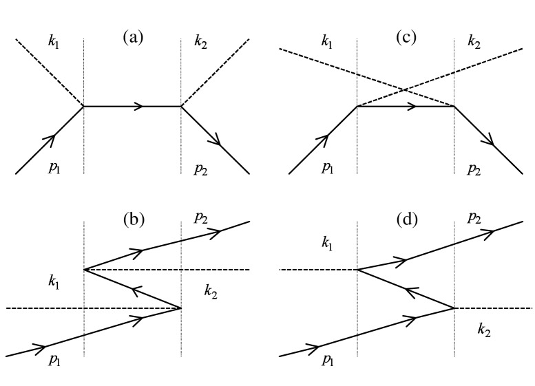
Figure 1: Different contributions to the $\pi N$ quasipotential within the Old-Fashioned Perturbation Theory (OFPT).

Such graphs are well-known from the old-fashioned perturbation theory (OFPT), where, for example, the $\pi N$ scattering $T$-matrix in the $g^{2}$-order is determined by the elements

$$\left\langle\mathbf{k}_{2},\mathbf{p}_{2}\mathbf{|}T^{\left(2\right)}(E+i0)\mathbf{|k}_{1},\mathbf{p}_{1}\right\rangle = \left\langle\mathbf{k}_{2},\mathbf{p}_{2}\mathbf{|}V(E+i0-H_{0})^{-1}V\mathbf{|k}_{1},\mathbf{p}_{1}\right\rangle$$

$$= \sum\limits_{i}\left\langle\mathbf{k}_{2},\mathbf{p}_{2}\mathbf{|}V\mathbf{|}i\right\rangle(E+i0-E_{i})^{-1}\left\langle i\mathbf{|}V\mathbf{|k}_{1},\mathbf{p}_{1}\right\rangle.$$

Here $E$ the collision energy and the summation is performed over all permissible intermediate states (the $H_{0}$ eigenstates) with energies $E_{i}$. In this context, the inverse energy denominators in the r.h.s. of Eq. (69) have the form $(E-E_{i})^{-1}$ with the appropriate values of $E$ and $E_{i}$. For example, $\left(E_{\mathbf{q}}+E_{\mathbf{p}_{1}}+\omega_{\mathbf{k}_{1}}\right)^{-1}$ and $\left(E_{\mathbf{p}_{2}}+E_{\mathbf{q}^{\prime}}-\omega_{\mathbf{k}_{1}}\right)^{-1}$ may be related to the noncovariant propagators

$$D^{-1}\left(E\right)|_{E=E_{\mathbf{p}_{2}}+\omega_{\mathbf{k}_{2}}} \equiv \left(E-E_{\mathbf{p}_{1}}-\omega_{\mathbf{k}_{1}}-E_{\mathbf{p}_{2}}-\omega_{\mathbf{k}_{2}}-E_{\mathbf{q}}\right)^{-1}|_{E=E_{\mathbf{p}_{2}}+\omega_{\mathbf{k}_{2}}}$$

$$= -\left(E_{\mathbf{q}}+E_{\mathbf{p}_{1}}+\omega_{\mathbf{k}_{1}}\right)^{-1},$$

and

$$\overline{D}^{-1}\left(E\right)|_{E=E_{\mathbf{p}_{1}}+\omega_{\mathbf{k}_{1}}} \equiv \left(E-E_{\mathbf{p}_{1}}-E_{\mathbf{p}_{2}}-E_{\mathbf{q}^{\prime}}\right)^{-1}|_{E=E_{\mathbf{p}_{1}}+\omega_{\mathbf{k}_{1}}}$$

$$= -\left(E_{\mathbf{p}_{2}}+E_{\mathbf{q}^{\prime}}-\omega_{\mathbf{k}_{1}}\right)^{-1},$$

being associated with the five and three internal lines putting in between the dotted verticals, respectively, in graphs $b$ and $d$. Both of them contain the $N\overline{N}$ pair in the intermediate states. Note that we have to distinguish the intermediate states of clothed particles in our approach from the intermediate states of bare particles with physical masses that usually appear in OFPT.

In addition, we would like to note that the graphs in Fig. 1 are topologically equivalent to the four time-ordered Feynman diagrams displayed in Fig. 20 in Chapter 13 of Schweber’s book SchweberBook . However, in the Schrödinger picture used here, where all events are related to one and the same instant $t=0$ the use of such an analogy seems to be misleading. In fact, the line directions in Fig. 1 are given with the sole scope to discriminate between the nucleon and antinucleon states.

The Feynman-like propagators in Eq. (66) appear after trivial transformations, e.g., adding the contribution $a$ and $b$, it is readily seen that

$$\frac{m}{E_{\mathbf{q}}}\left[\frac{\Lambda_{+}\left(q\right)}{E_{\mathbf{q}}-E_{\mathbf{p}_{1}}-\omega_{\mathbf{k}_{1}}}+\frac{\Lambda_{-}^{\dagger}\left(q\right)}{E_{\mathbf{q}}+E_{\mathbf{p}_{1}}+\omega_{\mathbf{k}_{1}}}\right]=-\frac{1}{\not{s}_{{}_{1}}-m},$$

where we have denoted the ”left” Mandelstam vector $s_{1}=\left(E_{\mathbf{p}_{1}}+\omega_{\mathbf{k}_{1}},\mathbf{p}_{1}+\mathbf{k}_{1}\right)=p_{1}+k_{1}$. Now, taking into account the property $\gamma_{5}\gamma_{\mu}\gamma_{5}=-\gamma_{\mu}$, one shortly derives Eq. (66).

We emphasize that energy conservation is not assumed in constructing this and other quasipotentials, and this forces us to give much more detailed and complicated expressions for these quasi-potentials. Indeed, the coefficients for the $a_{c}^{\dagger}b_{c}^{\dagger}a_{c}b_{c}$-terms appearing in the $K(\pi N\rightarrow\pi N)$ expansion generally do not fulfill the on-energy-shell condition

$$E_{\mathbf{p}_{1}}+\omega_{\mathbf{k}_{1}}=E_{\mathbf{p}_{2}}+\omega_{\mathbf{k}_{2}},$$ (70)

In this connection, the “left” four-vector $s_{1}$ is not necessarily equal to the ”right” Mandelstam vector $s_{2}=p_{2}+k_{2}$. Clearly, if the condition (70) is fulfilled, then $p_{1}-k_{2}=u$, so that the first (second) half-sum of the covariant propagators in the r.h.s. of Eq. (66) is converted into the $s$-pole ($u$-pole) propagator typical of Feynman technique. Thus, only the corresponding on-energy-shell part of the $\pi N$ quasipotential is represented in Fig. 2 by the genuine Feynman diagram.

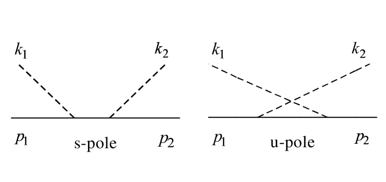
Figure 2: On-energy-shell contributions to the $\pi N$-quasipotential.

The quasipotential is nonlocal since the vertex factors and propagators in Eq. (66) are dependent not only on the relative three-momenta involved but also on their total three-momentum. Besides, this embodies the nonstatic (recoil) effects in all orders of the so-called $1/c^{2}$- expansion (see FoldyKrajcik ).

In the static limit, one can show that the off-energy-shell contributions differ from the on-energy-shell results by the values of the order $\mathbf{q}\,_{r}^{2}/\eta^{2}$ where $\mathbf{q}_{r}$ is the relative $\pi N$ momentum and $\eta=m\mu/(m+\mu)$ is the reduced $\pi N$ mass. One needs additional investigations to show to what extent these differences can be neglected when describing $\pi N$ scattering .

To our knowledge the formula (67) (albeit given in other form) has been first derived in ShirokovVisinescuRevRoumPhys1974 within the clothed particle approach.

The quasipotential determined by Eq. (66) has the same Feynman-like structure as the effective $\pi N$ interaction obtained in SatoLee.Phys.Rev.C54.2660.1996 (see the final formula below Eq. (A.8) therein). As mentioned in Introduction, the authors of SatoLee.Phys.Rev.C54.2660.1996 have used the other realization of UT method, which is similar to the Fröhlich transformation (see, e.g., Davydov1973 ) in the theory of metals.

In addition, one can show that the coefficients $V_{\pi N}(\mathbf{k}_{2},\mathbf{p}_{2};\mathbf{k}_{1},\mathbf{p}_{1})$ in Eq. (66) do not differ from those obtained in Ref. Fuda.Ann.Phys.231.1.1994 (after some simplifications of the model Hamiltonian used there). However, the corresponding pion-nucleon interaction operator from Ref. Fuda.Ann.Phys.231.1.1994 contains the bare particle $a^{\dagger}b^{\dagger}ab$-terms instead of the clothed particle $a_{c}^{\dagger}b_{c}^{\dagger}a_{c}b_{c}$-ones in our expression for $K(\pi N\rightarrow\pi N)$. It would be interesting and worthwhile to check if the same coincidence of results will be obtained for higher-order terms in the coupling constant.

III.3 Nucleon-nucleon interaction operator

After normal ordering of the fermion operators in the third integral in the r.h.s. of Eq. (63) and its Hermitian conjugate part the $NN\rightarrow NN$ interaction operator can be represented in the form:

$$K(NN\rightarrow NN)=\int d\mathbf{p}_{1}d\mathbf{p}_{2}d\mathbf{p}_{1}^{\prime}d\,\mathbf{p}_{2}^{\prime}V_{NN}(\mathbf{p}_{1}^{\prime},\mathbf{p}_{2}^{\prime};\mathbf{p}_{1},\mathbf{p}_{2})b_{c}^{\dagger}(\mathbf{p}_{1}^{\prime})b_{c}^{\dagger}(\mathbf{p}_{2}^{\prime})b_{c}(\mathbf{p}_{1})b_{c}(\mathbf{p}_{2}),$$

$$\vskip 3.0pt plus 1.0pt minus 1.0ptV_{NN}(\mathbf{p}_{1}^{\prime},\mathbf{p}_{2}^{\prime};\mathbf{p}_{1},\mathbf{p}_{2})=-\frac{1}{2}\frac{g^{2}}{(2\pi)^{3}}\frac{1}{2\omega_{\mathbf{p}_{1}^{\prime}-\mathbf{p}_{1}}}\frac{m^{2}}{\sqrt{E_{\mathbf{p}_{1}}E_{\mathbf{p}_{2}}E_{\mathbf{p}_{1}^{\prime}}E_{\mathbf{p}_{2}^{\prime}}}}\delta(\mathbf{p}_{1}^{\prime}+\mathbf{p}_{2}^{\prime}-\mathbf{p}_{1}-\mathbf{p}_{2})$$

$$\times\bar{u}(\mathbf{p}_{1}^{\prime})\gamma_{5}u(\mathbf{p}_{1})\left\{\frac{1}{E_{\mathbf{p}_{1}}-E_{\mathbf{p}_{1}^{\prime}}-\omega_{\mathbf{p}_{1}^{\prime}-\mathbf{p}_{1}}}+\frac{1}{E_{\mathbf{p}_{1}^{\prime}}-E_{\mathbf{p}_{1}}-\omega_{\mathbf{p}_{1}^{\prime}-\mathbf{p}_{1}}}\right\}\bar{u}(\mathbf{p}_{2}^{\prime})\gamma_{5}u(\mathbf{p}_{2})$$ (71)

As in case of the $\pi N$, we encounter here the noncovariant (“nonrelativistic”) propagators linear in the intermediate energies. It allows us to relate the two graphs in Fig. 3 to the r.h.s. of Eq. (71).

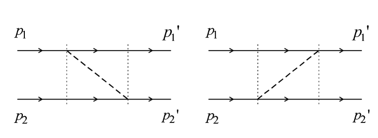
Figure 3: Illustration of Eq.(71) as a sum of two OFPT diagrams with the intermediate pion (dashed lines) on its mass shell.

The left and right diagrams in Fig.3 are associated with the OFPT denominators,

$$D\left(E\right)|_{E=E_{\mathbf{p}_{1}}+E_{\mathbf{p}_{2}}} \equiv \left(E-E_{\mathbf{p}_{1}^{\prime}}-E_{\mathbf{p}_{2}}-\omega_{\mathbf{p}_{1}^{\prime}-\mathbf{p}_{1}}\right)|_{E=E_{\mathbf{p}_{1}}+E_{\mathbf{p}_{2}}}$$

$$= E_{\mathbf{p}_{1}}-E_{\mathbf{p}_{1}^{\prime}}-\omega_{\mathbf{p}_{1}^{\prime}-\mathbf{p}_{1}}$$

and

$$\overline{D}\left(E\right)|_{E=E_{\mathbf{p}_{1}^{\prime}}+E_{\mathbf{p}_{2}^{\prime}}} \equiv \left(E-E_{\mathbf{p}_{1}}-E_{\mathbf{p}_{2}^{\prime}}-\omega_{\mathbf{p}_{2}^{\prime}-\mathbf{p}_{2}}\right)|_{E=E_{\mathbf{p}_{1}^{\prime}}+E_{\mathbf{p}_{2}^{\prime}}}$$

$$= E_{\mathbf{p}_{1}^{\prime}}-E_{\mathbf{p}_{1}}-\omega_{\mathbf{p}_{1}-\mathbf{p}_{1}^{\prime}},$$

respectively (cf. discussion in Sect. 3.2).

Though Eq.(71) is equivalent to

$$V_{NN}(\mathbf{p}_{1}^{\prime},\mathbf{p}_{2}^{\prime};\mathbf{p}_{1},\mathbf{p}_{2})=-\frac{1}{2}\frac{g^{2}}{(2\pi)^{3}}\frac{m^{2}}{\sqrt{E_{\mathbf{p}_{1}}E_{\mathbf{p}_{2}}E_{\mathbf{p}_{1}^{\prime}}E_{\mathbf{p}_{2}^{\prime}}}}\delta(\mathbf{p}_{1}^{\prime}+\mathbf{p}_{2}^{\prime}-\mathbf{p}_{1}-\mathbf{p}_{2})$$

$$\times\bar{u}(\mathbf{p}_{1}^{\prime})\gamma_{5}u(\mathbf{p}_{1})\frac{1}{(p_{1}-p_{1}^{\prime})^{2}-\mu^{2}}\bar{u}(\mathbf{p}_{2}^{\prime})\gamma_{5}u(\mathbf{p}_{2}),$$ (72)

the occurrence of such primary denominators is typical of the three-dimensional formalism developed here.

The corresponding relativistic and properly symmetrized $NN$ interaction, is given by the quasipotential

$$\tilde{V}_{NN}(\mathbf{p}_{1}^{\prime},\mathbf{p}_{2}^{\prime};\mathbf{p}_{1},\mathbf{p}_{2}) = \left\langle b_{c}^{\dagger}(\mathbf{p}_{1}^{\prime})b_{c}^{\dagger}(\mathbf{p}_{2}^{\prime})\Omega\mathbf{|}K(NN\rightarrow NN)\mathbf{|}b_{c}^{\dagger}(\mathbf{p}_{1})b_{c}^{\dagger}(\mathbf{p}_{2})\Omega\right\rangle$$ (73)

$$= \frac{1}{2}\left\{V_{NN}(\mathbf{p}_{1}^{\prime},\mathbf{p}_{2}^{\prime};\mathbf{p}_{1},\mathbf{p}_{2})-V_{NN}(\mathbf{p}_{1}^{\prime},\mathbf{p}_{2}^{\prime};\mathbf{p}_{2},\mathbf{p}_{1})\right.$$

$$\left.-V_{NN}(\mathbf{p}_{2}^{\prime},\mathbf{p}_{1}^{\prime};\mathbf{p}_{1},\mathbf{p}_{2})+V_{NN}(\mathbf{p}_{2}^{\prime},\mathbf{p}_{1}^{\prime};\mathbf{p}_{2},\mathbf{p}_{1})\right\},$$

(see formula (4.16) from Ref. SheShi2001 ).

Substituting (72) into (73), we express the quasipotential of interest through the covariant (Feynman-like) “propagators”,

$$\tilde{V}_{NN}(\mathbf{p}_{1}^{\prime},\mathbf{p}_{2}^{\prime};\mathbf{p}_{1},\mathbf{p}_{2})=-\frac{1}{2}\frac{g^{2}}{(2\pi)^{3}}\frac{m^{2}}{2\sqrt{E_{\mathbf{p}_{1}}E_{\mathbf{p}_{2}}E_{\mathbf{p}_{1}^{\prime}}E_{\mathbf{p}_{2}^{\prime}}}}\delta(\mathbf{p}_{1}^{\prime}+\mathbf{p}_{2}^{\prime}-\mathbf{p}_{1}-\mathbf{p}_{2})$$

$$\times\bar{u}(\mathbf{p}_{1}^{\prime})\gamma_{5}u(\mathbf{p}_{1})\frac{1}{2}\left\{\frac{1}{(p_{1}-p_{1}^{\prime})^{2}-\mu^{2}}+\frac{1}{(p_{2}-p_{2}^{\prime})^{2}-\mu^{2}}\right\}\bar{u}(\mathbf{p}_{2}^{\prime})\gamma_{5}u(\mathbf{p}_{2})-(1\leftrightarrow 2).$$ (74)

The r.h.s. of this equation consists of the “direct” term written explicitly and the “exchange” one $(1\leftrightarrow 2)$ with the prescription that the variables with label 1 and 2 should be mutually interchanged. Formula (74) determines the $NN$ part of an one-boson-exchange interaction derived via the Okubo transformation method in KorchinShebekoPhysAtNucl1993 (see also FudaZhang.Phys.Rev.C51.23.1995 ) taking into account the pion and heavy-meson exchanges.

As has been emphasized in Ref.KorchinShebekoPhysAtNucl1993 , a distinctive feature of potential (74) is the presence of a covariant (Feynman-like) “propagator”

$$\frac{1}{2}\left\{\frac{1}{(p_{1}-p_{1}^{\prime})^{2}-\mu^{2}}+\frac{1}{(p_{2}-p_{2}^{\prime})^{2}-\mu^{2}}\right\}\,.$$ (75)

On the energy shell for the $NN$ scattering, that is

$$E_{i}\equiv E_{\mathbf{p}_{1}}+E_{\mathbf{p}_{2}}=E_{\mathbf{p}_{1}^{\prime}}+E_{\mathbf{p}_{2}^{\prime}}\equiv E_{f},$$ (76)

this expression is converted into the genuine Feynman propagator which occurs when evaluating the $S$ - matrix for $NN$ scattering in the $g^{2}$-order. The corresponding graphs are displayed in Fig. 4. The quasipotential $\tilde{V}_{NN}$ can be related to these Feynman diagrams, being different from the corresponding Feynman $NN$-scattering amplitude in two respects, namely, $\tilde{V}_{NN}$ does not contain the factor $\delta(E_{\mathbf{p}_{1}}+E_{\mathbf{p}_{2}}-E_{\mathbf{p}_{1}^{\prime}}-E_{\mathbf{p}_{2}^{\prime}})$ and “propagator” (75) is now related to the meson line in the left graph in Fig. 4.

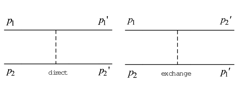
Figure 4: On-energy-shell contributions to the $NN$ interaction (the $g^{2}$-order Feynman diagrams for $NN$ scattering).

One could take this analysis a little further, and show that the off-energy-shell deviations from the conventional on-energy-shell result obtained in the static approximation are of the order $\mathbf{p}_{r}^{2}/m^{2}$, where $\mathbf{p}_{r}$ is the relative $NN$ momentum. In other words, the corresponding off-energy-shell corrections have a relativistic origin.

Explicit formulae for the $NN$-quasipotential generated by the exchange of heavier mesons are given in the next section.

III.4 $NN\leftrightarrow\pi NN$ transition operators

To separate the $NN\leftrightarrow\pi NN$ interaction operators one needs to perform the normal ordering of fermion operators in the fourth and fifth integrals of Eq. (64) and their Hermitian conjugate parts. After a lengthy algebra we get the pion production operator,

$$K(NN \rightarrow \pi NN)=\int d\mathbf{p}_{1}d\mathbf{p}_{2}d\mathbf{p}_{1}^{\prime}d\mathbf{p}_{2}^{\prime}d\mathbf{k}V_{\pi NN}(\mathbf{p}_{1}^{\prime},\mathbf{p}_{2}^{\prime},\mathbf{k};\mathbf{p}_{1},\mathbf{p}_{2})$$ (77)

$$\times a_{c}^{\dagger}(\mathbf{k})b_{c}^{\dagger}(\mathbf{p}_{1}^{\prime})b_{c}^{\dagger}(\mathbf{p}_{2}^{\prime})b_{c}(\mathbf{p}_{1})b_{c}(\mathbf{p}_{2}),$$

$$V_{\pi NN}\left(\mathbf{{p}_{1}^{\prime},{p}_{2}^{\prime},{k};{p}_{1},{p}_{2}}\right)=V_{\pi NN}\left(\mathrm{Feynman-like}\right)+V_{\pi NN}\left(\mathrm{off-energy-shell}\right),$$

where

$$V_{\pi NN}(\mathrm{Feynman-like})=-i\frac{g^{3}}{(2\pi)^{9/2}}\frac{m^{2}}{\sqrt{2\omega_{\mathbf{k}}E_{\mathbf{p}_{1}}E_{\mathbf{p}_{2}}E_{\mathbf{p}_{1}^{\prime}}E_{\mathbf{p}_{2}^{\prime}}}}\delta(\mathbf{p}_{1}+\mathbf{p}_{2}-\mathbf{p}_{1}^{\prime}-\mathbf{p}_{2}^{\prime}-\mathbf{k})$$

$$\times\frac{\bar{u}(\mathbf{p}_{2}^{\prime})\gamma_{5}u(\mathbf{p}_{2})}{(p_{2}-p_{2}^{\prime})^{2}-\mu^{2}}\bar{u}(\mathbf{p}_{1}^{\prime})\left[\frac{1}{\not{p}_{1}^{\prime}+\not{k}+m}+\frac{1}{\not{p}_{1}-\not{k}+m}\right]u(\mathbf{p}_{1}),$$ (78)

and

$$V_{\pi NN}(\mathrm{off-energy-shell})=-i\frac{1}{3}\frac{g^{3}}{(2\pi)^{9/2}}\frac{m^{2}}{\sqrt{2\omega_{\mathbf{k}}E_{\mathbf{p}_{1}}E_{\mathbf{p}_{2}}E_{\mathbf{p}_{1}^{\prime}}E_{\mathbf{p}_{2}^{\prime}}}}\delta(\mathbf{p}_{1}+\mathbf{p}_{2}-\mathbf{p}_{1}^{\prime}-\mathbf{p}_{2}^{\prime}-\mathbf{k})$$

$$\times\frac{\bar{u}(\mathbf{p}_{2}^{\prime})\gamma_{5}u(\mathbf{p}_{2})}{2\omega_{\mathbf{p}_{2}-\mathbf{p}_{2}^{\prime}}}\left\{\left(\frac{1}{E_{\mathbf{p}_{2}}-E_{\mathbf{p}_{2}^{\prime}}+\omega_{\mathbf{p}_{2}-\mathbf{p}_{2}^{\prime}}}-\frac{1}{E_{\mathbf{p}_{1}^{\prime}}+\omega_{\mathbf{k}}-E_{\mathbf{p}_{1}}+\omega_{\mathbf{p}_{2}-\mathbf{p}_{2}^{\prime}}}\right)\right.$$

$$\times\bar{u}(\mathbf{p}_{1}^{\prime})\left[\frac{1}{\not{p}_{1}^{\prime}+\not{k}+m}+\frac{1}{\not{p}_{1}-\not{k}+m}\right]u(\mathbf{p}_{1})$$

$$-\left(\frac{1}{E_{\mathbf{p}_{2}}-E_{\mathbf{p}_{2}^{\prime}}-\omega_{\mathbf{p}_{2}-\mathbf{p}_{2}^{\prime}}}-\frac{1}{E_{\mathbf{p}_{1}^{\prime}}+\omega_{\mathbf{k}}-E_{\mathbf{p}_{1}}-\omega_{\mathbf{p}_{2}-\mathbf{p}_{2}^{\prime}}}\right)$$

$$\times\bar{u}(\mathbf{p}_{1}^{\prime})\left[\frac{1}{\not{p}_{1}^{\prime}+\not{k}+m}+\frac{1}{\not{p}_{1}-\not{k}+m}\right]u(\mathbf{p}_{1})$$

$$\left.+\left(\frac{1}{E_{\mathbf{p}_{2}}-E_{\mathbf{p}_{2}^{\prime}}-\omega_{\mathbf{p}_{2}-\mathbf{p}_{2}^{\prime}}}-\frac{1}{E_{\mathbf{p}_{1}^{\prime}}+\omega_{\mathbf{k}}-E_{\mathbf{p}_{1}}-\omega_{\mathbf{p}_{2}-\mathbf{p}_{2}^{\prime}}}\right)\right.$$

$$\times\bar{u}(\mathbf{p}_{1}^{\prime})\left[\frac{1}{\not{p}_{1}+\not{q}+m}+\frac{1}{\not{p}_{1}^{\prime}-\not{q}+m}\right]u(\mathbf{p}_{1})$$

$$-\left(\frac{1}{E_{\mathbf{p}_{2}}-E_{\mathbf{p}_{2}^{\prime}}+\omega_{\mathbf{p}_{2}-\mathbf{p}_{2}^{\prime}}}-\frac{1}{E_{\mathbf{p}_{1}^{\prime}}+\omega_{\mathbf{k}}-E_{\mathbf{p}_{1}}+\omega_{\mathbf{p}_{2}-\mathbf{p}_{2}^{\prime}}}\right)$$

$$\times\left.\bar{u}(\mathbf{p}_{1}^{\prime})\left[\frac{1}{\not{p}_{1}^{\prime}+\not{q}\_+m}+\frac{1}{\not{p}_{1}-\not{q}\_+m}\right]u(\mathbf{p}_{1})\right\}$$ (79)

with $q=p_{2}-p_{2}^{\prime}$ and $q\_=(\omega_{\bf q},-{\bf q})$.

We have used the relation

$$\left[(x-y)^{2}-\mu^{2}\right]^{-1}=\frac{1}{\omega_{\mathbf{x}-\mathbf{y}}}\left(\left[x_{0}-y_{0}-\omega_{\mathbf{x}-\mathbf{y}}\right]^{-1}-\left[x_{0}-y_{0}+\omega_{\mathbf{x}-\mathbf{y}}\right]^{-1}\right),$$ (80)

that holds for any four-vectors $x=(x_{0},\mathbf{x})$ and $y=(y_{0},\mathbf{y})$ with $\omega_{\mathbf{z}}=\sqrt{\mathbf{z}^{2}+\mu^{2}}$.

On the energy shell:

$$E_{\mathbf{p}_{1}}+E_{\mathbf{p}_{2}}=E_{\mathbf{p}_{1}^{\prime}}+E_{\mathbf{p}_{2}^{\prime}}+\omega_{\mathbf{k}}$$ (81)

expression (78) yields the pion production $T$ matrix in the $g^{3}$-order, i.e., to the first nonvanishing approximation in the CPR. We remind that a clothed pion cannot be absorbed or emitted by a clothed nucleon. At the same time the r.h.s. of (79) becomes equal to zero since under condition (81 ) the propagators in its round brackets cancel each other.

By analogy with the interaction between clothed nucleons we could introduce a quasipotential defined by the matrix elements of the operator (77) between the properly symmetrized clothed $NN$ and $\pi NN$ states

$$\tilde{V}_{\pi NN}(\mathbf{p}_{1}^{\prime},\mathbf{p}_{2}^{\prime},\mathbf{k};\mathbf{p}_{1},\mathbf{p}_{2})=\left\langle a_{c}^{\dagger}(\mathbf{k})b_{c}^{\dagger}(\mathbf{p}_{1}^{\prime})b_{c}^{\dagger}(\mathbf{p}_{2}^{\prime})\Omega\mathbf{|}K(NN\rightarrow\pi NN)\mathbf{|}b_{c}^{\dagger}(\mathbf{p}_{1})b_{c}^{\dagger}(\mathbf{p}_{2})\Omega\right\rangle$$

$$=\frac{1}{2}\left\{V_{\pi NN}(\mathbf{p}_{1}^{\prime},\mathbf{p}_{2}^{\prime},\mathbf{k};\mathbf{p}_{1},\mathbf{p}_{2})-V_{\pi NN}(\mathbf{p}_{1}^{\prime},\mathbf{p}_{2}^{\prime},\mathbf{k};\mathbf{p}_{2},\mathbf{p}_{1})\right.$$

$$\left.-V_{\pi NN}(\mathbf{p}_{2}^{\prime},\mathbf{p}_{1}^{\prime},\mathbf{k};\mathbf{p}_{1},\mathbf{p}_{2})+V_{\pi NN}(\mathbf{p}_{2}^{\prime},\mathbf{p}_{1}^{\prime},\mathbf{k};\mathbf{p}_{2},\mathbf{p}_{1})\right\}$$ (82)

Of course, such matrix elements characterize only some part of that physical input which contributes to pion-nuclear dynamics with the operator (77) included in the interaction $K_{I}$.

All the terms involved in the  $V_{\pi NN}$ quasipotential may be divided into the two groups. The first group refers to the pion production mechanisms shown schematically in Fig. 5.

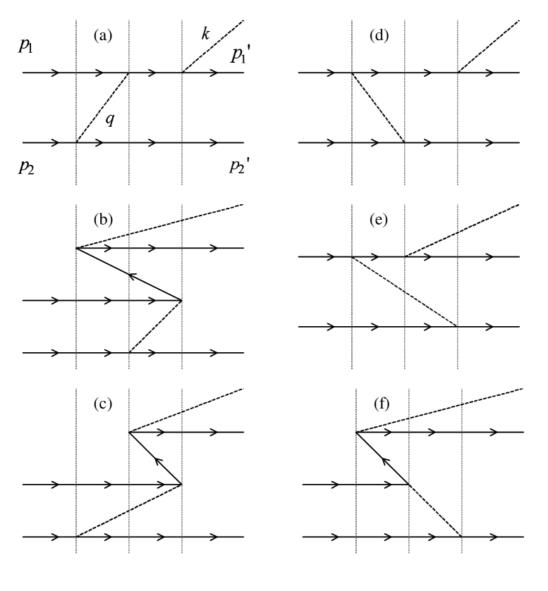
Figure 5: Illustration of the “retarded” pion production mechanisms on the $NN$ pair in the  $g^{3}$-order.

Note that the three left graphs in Fig. 5 exemplify the processes in which the pion created by one nucleon is scattered by another one, while the three graphs on the r.h.s. show the processes, where one nucleon emits two pions one of which is absorbed by another nucleon. Again, on the energy shell the sum of all these contributions can be represented by the Feynman graph (Fig. 6, left) with the pion exchange preceding the pion emission.

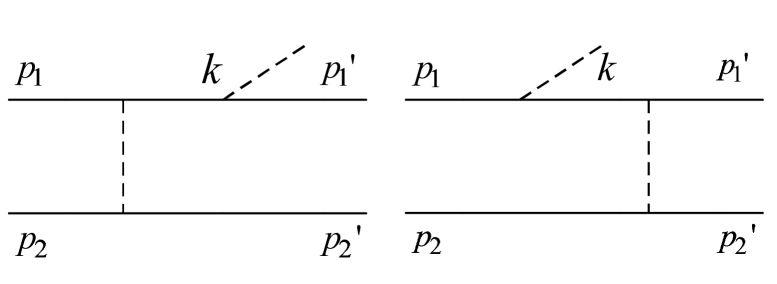
Figure 6: The conventional Feynman diagrams for the $NN\rightarrow\pi NN$ process in the $g^{3}$–order.

The second group of terms which could be extracted from Eqs. (78) and (79) are shown in Fig. 7.

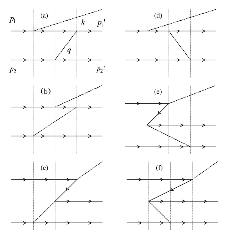
Figure 7: Illustration of the “advanced” pion production mechanisms on the $NN$ pair in the  $g^{3}$-order.

On the energy shell, the sum of these contributions can be represented by the Feynman graph (Fig. 6, right) with the pion emission preceding the pion exchange. Therefore, in the first nonvanishing approximation a pion can be absorbed/emitted only by a correlated $NN$ pair through a mechanism of the $g^{3}$-order.

In Ref. KobayashiSatoOhtsuboProgrTheorPhys1997 the UT method has been applied to the same $NN\rightarrow\pi NN$ process assuming a meson-nucleon PV-coupling. Taking into account this difference in the coupling scheme and relying upon our Eqs. (78) and (79), one can reproduce those effective interactions given first in KobayashiSatoOhtsuboProgrTheorPhys1997 .

In search of physical interpretation of the obtained results let us consider the expression

$$\frac{\bar{u}(\mathbf{p}_{2}^{\prime})\gamma_{5}u(\mathbf{p}_{2})}{E_{\mathbf{p}_{2}}-E_{\mathbf{p}_{2}^{\prime}}-\omega_{\mathbf{p}_{2}-\mathbf{p}_{2}^{\prime}}}\bar{u}(\mathbf{p}_{1}^{\prime})\left[\frac{1}{\not{p}_{1}^{\prime}+\not{k}+m}+\frac{1}{\not{p}_{1}-\not{k}+m}\right]u(\mathbf{p}_{1}).$$ (83)

We could write

$$\left[E_{\mathbf{p}_{2}}-E_{\mathbf{p}_{2}^{\prime}}-\omega_{\mathbf{p}_{2}-\mathbf{p}_{2}^{\prime}}\right]^{-1}=\left[E-E_{\mathbf{p}_{1}}-E_{\mathbf{p}_{2}^{\prime}}-\omega_{\mathbf{p}_{2}-\mathbf{p}_{2}^{\prime}}\right]^{-1}$$

with $E=E_{\mathbf{p}_{1}}+E_{\mathbf{p}_{2}}$ that is prompted with the graphical representation of (83) (more exactly, its part) in Fig. 8a, where all vertices displayed by circles (”interaction points”) are connected by bold lines (among them the nucleon line has the right arrow to distinguish nucleons and antinucleons).

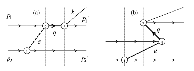
Figure 8: Graphical representation of Eqs. (83).

As admitted in the OFPT, the particle three-momenta are related to the lines in Fig. 8a via the following prescription: when moving from the left to the right, a sum of ”outgoing” momenta is equal to a sum of ”ingoing” ones. Here the term ”ingoing” (”outgoing”) is referred to the corresponding line or lines lying on the left (right) from the dotted vertical (a ”phantom” line) that passes through a given vertex. These vertices and phantoms are enumerated in the alphabetical order 1, 2, 3, … Accordingly, we have

$$\mathbf{p}_{2}=\mathbf{e}+\mathbf{p}_{2}^{\prime},\,\,\,\,\,\,\,\,\,\mathbf{p}_{1}+\mathbf{e}=\mathbf{q}=\mathbf{k}+\mathbf{p}_{1}^{\prime}.$$ (84)

Evidently, being taken together, these equations provide the total momentum conservation,

$$\mathbf{p}_{1}+\mathbf{p}_{2}=\mathbf{k}+\mathbf{p}_{1}^{\prime}+\mathbf{p}_{2}^{\prime}.$$ (85)

In parallel, we could consider Fig. 8b, where $\mathbf{p}_{2}=\mathbf{e}+\mathbf{p}_{2}^{\prime}$, $\mathbf{e}+\mathbf{p}_{1}+\mathbf{q}=0$ and $\mathbf{q}+\mathbf{p}_{1}^{\prime}+\mathbf{k}=0$. In particular, it means that $-\mathbf{q}=\mathbf{p}_{1}^{\prime}+\mathbf{k}=\mathbf{e}+\mathbf{p}_{1}=\mathbf{p}_{2}-\mathbf{p}_{2}^{\prime}$ in accordance with (85).

As in case of Fig. 8a, the three internal lines between the phantoms 1 and 2 can be associated with the OFPT propagator, $\left[E_{\mathbf{p}_{2}}-E_{\mathbf{p}_{2}^{\prime}}-\omega_{\mathbf{p}_{2}-\mathbf{p}_{2}^{\prime}}\right]^{-1}$.

Regarding the lines between the phantoms 2 and 3 in Fig. 8a and Fig. 8b one can make up the propagators (cf. discussion in Sect. 3.2)

$$\frac{1}{E-E_{\mathbf{q}}-E_{\mathbf{p}_{2}^{\prime}}}|_{E=E_{\mathbf{p}_{1}^{\prime}}+E_{\mathbf{p}_{2}^{\prime}}+\omega_{\mathbf{k}}}=\frac{1}{E_{\mathbf{p}_{1}^{\prime}}-E_{\mathbf{q}}+\omega_{\mathbf{k}}}$$ (86)

and

$$\left[E-\omega_{\mathbf{k}}-E_{\mathbf{p}_{1}^{\prime}}-E_{\mathbf{q}}-E_{\mathbf{p}_{1}}-E_{\mathbf{p}_{2}^{\prime}}-\omega_{\mathbf{p}_{2}-\mathbf{p}_{2}^{\prime}}\right]^{-1}=-\,\,\,\left[E_{\mathbf{p}_{1}^{\prime}}+\omega_{\mathbf{k}}+E_{\mathbf{q}}\right]^{-1}$$ (87)

with $E=E_{\mathbf{p}_{1}}+E_{\mathbf{p}_{2}^{\prime}}+\omega_{\mathbf{p}_{2}-\mathbf{p}_{2}^{\prime}}$ .

Handling the off-energy-shell graphs such as in Figs. 8a and 8b we cannot a priori ignore another option: with $E=E_{\mathbf{p}_{1}}+E_{\mathbf{p}_{2}^{\prime}}+\omega_{\mathbf{p}_{2}-\mathbf{p}_{2}^{\prime}}$ in (86) and $E=E_{\mathbf{p}_{1}^{\prime}}+E_{\mathbf{p}_{2}^{\prime}}+\omega_{\mathbf{k}}$ in (87). Both options contribute to the r.h.s. of (79), being equal to each other on the energy shell.

Doing so and using the well-known rules, where, for instance, the vertices with the lable 2 in Fig. 8a and Fig. 8b are equivalent to the factors

$$i\frac{g}{\sqrt{2\left(2\pi\right)^{3}\omega_{\mathbf{p}_{2}-\mathbf{p}_{2}^{\prime}}}}\frac{m}{\sqrt{E_{\mathbf{p}_{1}}E_{\mathbf{q}}}}\bar{u}(\mathbf{q})\gamma_{5}u(\mathbf{p}_{1})$$ (88)

and

$$i\frac{g}{\sqrt{2\left(2\pi\right)\omega_{\mathbf{k}}}}\frac{m}{\sqrt{E_{\mathbf{p}_{1}^{\prime}}E_{\mathbf{q}}}}\bar{u}(\mathbf{p}_{1}^{\prime})\gamma_{5}u(\mathbf{q}),$$ (89)

respectively, it is easy to get the matrix element

$$\bar{u}(\mathbf{p}_{1}^{\prime})\left[\not{p}_{1}^{\prime}+\not{k}+m\right]^{-1}u(\mathbf{q})$$ (90)

typical of the single-nucleon matrix elements involved in (78) and (79).

Relying upon the discussion below (70) one may say that the quantity (90) is related to the ”right-hand” $s$-pole mechanism of the off-energy-shell scattering of the intermediate meson (pion), that has been emitted by nucleon 2, on nucleon 1.

As in Subsects. 3.2-3.3, one has to stress again that, unlike the Feynman diagrams in Fig. 6, the meson is on its mass shell. Being a mediator in forming different pion production mechanisms on the correlated pair of nucleons, it is intimately embedded in the diagram of Fig. 9a, where, first, one of the interacting nucleons ”shakes off” the pion (the bright spot) which is absorbed, then, by the other nucleon (the hatched spot) with the subsequent (”retarded”) emission of the detected meson (pion).

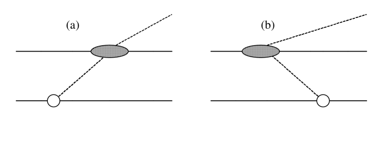
Figure 9: Graphical representation for the “retarded” (a) and “advanced” (b) pion production mechanisms on the $NN$ pair.

Of course, such ”chronological” expressions which employ the terms ”first” and ”then” has nothing common with any real time development of the process $NN\leftrightarrow\pi NN$. In fact, we imply a left-to-right-hand alignment of intermediate pion-fermion states that occur when evaluating the matrix elements $\left\langle\pi NN|V|n\right\rangle\left\langle n|V|m\right\rangle\left\langle m|V|NN\right\rangle$, where $\left|m\right\rangle$ and $\left|n\right\rangle$ are permissible $K_{F}$ eigenstates. In this respect, it is useful to keep in mind the on-energy-shell relationship

$$\left\langle\pi NN|{\frac{1}{3}}\left[R,\left[R,V\right]\right]|NN\right\rangle=\left\langle\pi NN|VG_{F}\left(E\right)VG_{F}\left(E\right)V|NN\right\rangle$$

with the resolvent expressed by

$$G_{F}\left(E\right)=\left(E-K_{F}\right)^{-1}$$

$$E=E_{\mathbf{p}_{1}}+E_{\mathbf{p}_{2}}=E_{\mathbf{p}_{1}^{\prime}}+E_{\mathbf{p}_{2}^{\prime}}+\omega_{\mathbf{k}}.$$

Nevertheless, it is convenient to refer to the reaction mechanisms represented in Fig. 9a as ”retarded”, to differentiate them from the ”advanced” ones displayed in Fig. 9b.

IV Incorporation of heavy-meson exchanges

In this section we have collected our more general evaluations of quasipotentials for the $NN\rightarrow NN$ and $NN\rightarrow\pi NN$ interactions that are due to the exchange of $b=\pi,\eta,\rho,\omega,\delta$ and $\sigma$ mesons.

IV.1 Pion and heavier-meson exchanges in $NN\rightarrow NN$ process

Here we consider the well-known Yukawa-type meson-nucleon couplings (see, e.g., FudaZhang.Phys.Rev.C54.495.1996 ) additively involved in the primary total Hamiltonian. Application of our approach in this case results in the following expression for the $NN\rightarrow NN$ quasipotential

$$\tilde{V}_{NN}(\mathbf{p}_{1}^{\prime},\mathbf{p}_{2}^{\prime};\mathbf{p}_{1},\mathbf{p}_{2})=-\frac{1}{2(2\pi)^{3}}\frac{m^{2}}{\sqrt{E_{\mathbf{p}_{1}}E_{\mathbf{p}_{2}}E_{\mathbf{p}_{1}^{\prime}}E_{\mathbf{p}_{2}^{\prime}}}}\delta(\mathbf{p}_{1}^{\prime}+\mathbf{p}_{2}^{\prime}-\mathbf{p}_{1}-\mathbf{p}_{2})$$

$$\times\sum_{b}\tilde{V}_{NN}^{b}(\mathbf{p}_{1}^{\prime},\mathbf{p}_{2}^{\prime};\mathbf{p}_{1},\mathbf{p}_{2}).$$ (91)

The contribution to this formula from the $\delta$- and $\sigma$- mesons exchange is given by

$$\tilde{V}_{NN}^{b}(\mathbf{p}_{1}^{\prime},\mathbf{p}_{2}^{\prime};\mathbf{p}_{1},\mathbf{p}_{2})=g_{b}^{2}h_{b}\frac{\bar{u}(\mathbf{p}_{1}^{\prime})u(\mathbf{p}_{1})\bar{u}(\mathbf{p}_{2}^{\prime})u(\mathbf{p}_{2})}{(p_{1}-p_{1}^{\prime})^{2}-\mu_{b}^{2}}$$

$$+(1\leftrightarrow 2,1^{\prime}\leftrightarrow 2^{\prime})-(1\leftrightarrow 2)-(1^{\prime}\leftrightarrow 2^{\prime}),b=\delta,\sigma,\,\,\,h_{\delta}=\mathbf{\tau}_{1}\cdot\mathbf{\tau}_{2},h_{\sigma}=1.$$ (92)

As usually, the Pauli vector $\mathbf{\tau}$ is the matrix in the nucleon isospin space. The account for the $\pi$- and $\eta$- mesons exchange gives rise to the following contribution

$$\tilde{V}_{NN}^{b}(\mathbf{p}_{1}^{\prime},\mathbf{p}_{2}^{\prime};\mathbf{p}_{1},\mathbf{p}_{2})=g_{b}^{2}h_{b}\frac{\bar{u}(\mathbf{p}_{1}^{\prime}\,r_{1}^{\prime})\gamma_{5}u(\mathbf{p}_{1}\,r_{1})\bar{u}(\mathbf{p}_{2}^{\prime}\,r_{2}^{\prime})\gamma_{5}u(\mathbf{p}_{2}\,r_{2})}{(p_{1}-p_{1}^{\prime})^{2}-\mu_{b}^{2}}$$

$$+(1\leftrightarrow 2,1^{\prime}\leftrightarrow 2^{\prime})-(1\leftrightarrow 2)-(1^{\prime}\leftrightarrow 2^{\prime}),b=\pi,\eta,\,\,\,h_{\pi}=\mathbf{\tau}_{1}\cdot\mathbf{\tau}_{2},h_{\eta}=1.$$ (93)

At last, the $NN$ quasipotential originating from the $\rho$- and $\omega$- mesons exchange can be written as

$$\tilde{V}_{NN}^{b}(\mathbf{p}_{1}^{\prime},\mathbf{p}_{2}^{\prime};\mathbf{p}_{1},\mathbf{p}_{2})=g_{b}^{2}h_{b}\frac{\bar{u}(\mathbf{p}_{1}^{\prime})\gamma_{\mu}u(\mathbf{p}_{1})\Lambda_{b}^{\mu\nu}(p_{1}-p_{1}^{\prime})\bar{u}(\mathbf{p}_{2}^{\prime})\gamma_{\nu}u(\mathbf{p}_{2})}{(p_{1}-p_{1}^{\prime})^{2}-\mu_{b}^{2}}$$

$$+(1\leftrightarrow 2,1^{\prime}\leftrightarrow 2^{\prime})-(1\leftrightarrow 2)-(1^{\prime}\leftrightarrow 2^{\prime}),$$

$$b=\rho,\omega,\,\,\,h_{\rho}=\mathbf{\tau}_{1}\cdot\mathbf{\tau}_{2},h_{\omega}=1,\Lambda_{b}^{\mu\nu}(q)=-g^{\mu\nu}+(q^{\mu}q^{\nu}/\mu_{b}^{2}).$$ (94)

IV.2 Heavy-meson exchanges in $NN\leftrightarrow\pi NN$ processes

In regards to the $NN\leftrightarrow\pi NN$ process the corresponding quasipotential has the form

$$\tilde{V}_{\pi NN}(\mathbf{p}_{1}^{\prime}\,r_{1}^{\prime},\mathbf{p}_{2}^{\prime}\,r_{2}^{\prime},\mathbf{k};\mathbf{p}_{1}\,r_{1},\mathbf{p}_{2}\,r_{2})=\frac{im^{2}}{3(2\pi)^{9/2}}\frac{\delta(\mathbf{p}_{1}+\mathbf{p}_{2}-\mathbf{p}_{1}^{\prime}-\mathbf{p}_{2}^{\prime}-\mathbf{k})}{\sqrt{E_{\mathbf{p}_{1}}E_{\mathbf{p}_{1}^{\prime}}E_{\mathbf{p}_{2}}E_{\mathbf{p}_{2}^{\prime}}}}$$

$$\times\sum_{b,j}\frac{1}{\sqrt{2\omega_{\mathbf{k}}^{j}}}\tilde{V}_{\pi NN}^{b,j}(\mathbf{p}_{1}^{\prime}\,r_{1}^{\prime},\mathbf{p}_{2}^{\prime}\,r_{2}^{\prime},\mathbf{k};\mathbf{p}_{1}\,r_{1},\mathbf{p}_{2}\,r_{2}).$$ (95)

The $\delta$- and $\sigma$- mesons exchange contribution to this formula is given by

$$\tilde{V}_{\pi NN}^{b,j}(\mathbf{p}_{1}^{\prime},\mathbf{p}_{2}^{\prime},\mathbf{k};\mathbf{p}_{1},\mathbf{p}_{2})=g_{\pi}g_{b}^{2}\bar{u}(\mathbf{p}_{2}^{\prime})u(\mathbf{p}_{2})\bar{u}(\mathbf{p}_{1}^{\prime})$$

$$\times\left\{\left[-\frac{2}{q^{2}-\mu_{b}^{2}}+\frac{1}{(p_{1}^{\prime}+k-p_{1})^{2}-\mu_{b}^{2}}\right]\left[\frac{t_{b,1}^{j}}{\not{p}_{1}^{\prime}+\not{k}+m}-\frac{t_{b,2}^{j}}{\not{p}_{1}-\not{k}-m}\right]\right.$$

$$\left.+\frac{1}{2\omega_{q}^{b}}\left[\frac{1}{E_{\mathbf{p}_{2}}-E_{\mathbf{p}_{2}^{\prime}}-\omega_{q}^{b}}+\frac{1}{E_{\mathbf{p}_{1}}-E_{\mathbf{p}_{1}^{\prime}}+\omega_{q}^{b}-\omega_{\mathbf{k}}^{j}}\right]\left[-\frac{t_{b,1}^{j}}{\not{p}_{1}+\not{q}+m}+\frac{t_{b,2}^{j}}{\not{p}_{1}^{\prime}-\not{q}-m}\right]\right.$$

$$\left.+\frac{1}{2\omega_{q}^{b}}\left[\frac{1}{E_{\mathbf{p}_{2}^{\prime}}-E_{\mathbf{p}_{2}}-\omega_{q}^{b}}+\frac{1}{E_{\mathbf{p}_{1}^{\prime}}-E_{\mathbf{p}_{1}}+\omega_{q}^{b}+\omega_{\mathbf{k}}^{j}}\right]\left[\frac{t_{b,2}^{j}}{\not{p}_{1}^{\prime}+\not{q}\_-m}-\frac{t_{b,1}^{j}}{\not{p}_{1}-\not{q}\_+m}\right]\right\}$$

$$\times\gamma_{5}u(\mathbf{p}_{1}\,r_{1})+(1\leftrightarrow 2,1^{\prime}\leftrightarrow 2^{\prime})-(1\leftrightarrow 2)-(1^{\prime}\leftrightarrow 2^{\prime}),$$

$$b=\delta,\sigma,\,\,\,t_{\delta,1}^{j}=\tau_{1}^{j}\mathbf{\tau}_{1}\mathbf{\tau}_{2},\,\,\,t_{\delta,2}^{j}=\mathbf{\tau}_{2}\mathbf{\tau}_{1}\tau_{1}^{j},\,\,\,t_{\sigma,1}^{j}=t_{\sigma,2}^{j}=1^{j}.$$ (96)

The $\pi$- and $\eta$- mesons exchange gives the contribution

$$\tilde{V}_{\pi NN}^{b,j}(\mathbf{p}_{1}^{\prime}\,r_{1}^{\prime},\mathbf{p}_{2}^{\prime}\,r_{2}^{\prime},\mathbf{k};\mathbf{p}_{1}\,r_{1},\mathbf{p}_{2}\,r_{2})=g_{\pi}g_{b}^{2}\bar{u}(\mathbf{p}_{2}^{\prime}\,r_{2}^{\prime})\gamma_{5}u(\mathbf{p}_{2}\,r_{2})\bar{u}(\mathbf{p}_{1}^{\prime}\,r_{1}^{\prime})$$

$$\times\left\{\left[\frac{2}{q^{2}-\mu_{b}^{2}}+\frac{1}{(p_{1}^{\prime}+k-p_{1})^{2}-\mu_{b}^{2}}\right]\left[\frac{t_{b,1}^{j}}{\not{p}_{1}^{\prime}+\not{k}+m}+\frac{t_{b,2}^{j}}{\not{p}_{1}-\not{k}+m}\right]\right.$$

$$\left.+\frac{1}{2\omega_{q}^{b}}\left[\frac{1}{E_{\mathbf{p}_{2}}-E_{\mathbf{p}_{2}^{\prime}}-\omega_{q}^{b}}+\frac{1}{E_{\mathbf{p}_{1}}-E_{\mathbf{p}_{1}^{\prime}}+\omega_{q}^{b}-\omega_{\mathbf{k}}^{j}}\right]\left[\frac{t_{b,1}^{j}}{\not{p}_{1}+\not{q}+m}+\frac{t_{b,2}^{j}}{\not{p}_{1}^{\prime}-\not{q}+m}\right]\right.$$

$$\left.+\frac{1}{2\omega_{q}^{b}}\left[\frac{1}{E_{\mathbf{p}_{2}^{\prime}}-E_{\mathbf{p}_{2}}-\omega_{q}^{b}}+\frac{1}{E_{\mathbf{p}_{1}^{\prime}}-E_{\mathbf{p}_{1}}+\omega_{q}^{b}+\omega_{\mathbf{k}}^{j}}\right]\left[\frac{t_{b,2}^{j}}{\not{p}_{1}^{\prime}+\not{q}\_+m}+\frac{t_{b,1}^{j}}{\not{p}_{1}-\not{q}\_+m}\right]\right\}$$

$$\times u(\mathbf{p}_{1})+(1\leftrightarrow 2,1^{\prime}\leftrightarrow 2^{\prime})-(1\leftrightarrow 2)-(1^{\prime}\leftrightarrow 2^{\prime}),$$

$$b=\pi,\eta,\,\,\,t_{\pi,1}^{j}=\tau_{1}^{j}\mathbf{\tau}_{1}\mathbf{\tau}_{2},\,\,\,t_{\pi,2}^{j}=\mathbf{\tau}_{2}\mathbf{\tau}_{1}\tau_{1}^{j},\,\,\,t_{\eta,1}^{j}=t_{\eta,2}^{j}=1^{j}.$$ (97)

Finally, the $\pi NN$ quasipotential originating from the $\rho$- and $\omega$- mesons exchange is determined by

$$\tilde{V}_{\pi NN}^{b,j}(\mathbf{p}_{1}^{\prime}\,r_{1}^{\prime},\mathbf{p}_{2}^{\prime}\,r_{2}^{\prime},\mathbf{k};\mathbf{p}_{1}\,r_{1},\mathbf{p}_{2}\,r_{2})=g_{\pi}g_{b}^{2}\bar{u}(\mathbf{p}_{2}^{\prime}\,r_{2}^{\prime})\gamma_{\mu}u(\mathbf{p}_{2}\,r_{2})\Lambda_{b}^{\mu\nu}(p_{2}-p_{2}^{\prime})\bar{u}(\mathbf{p}_{1}^{\prime}\,r_{1}^{\prime})$$

$$\times\left\{\left[\frac{2}{q^{2}-\mu_{b}^{2}}+\frac{1}{(p_{1}^{\prime}+k-p_{1})^{2}-\mu_{b}^{2}}\right]\left[-\frac{t_{b,1}^{j}\gamma_{\nu}}{\not{p}_{1}^{\prime}+\not{k}+m}+\frac{t_{b,2}^{j}\gamma_{\nu}}{\not{p}_{1}-\not{k}+m}-\frac{2t_{b,2}^{j}(p_{1}-k)_{\nu}}{(p_{1}-k)^{2}-m^{2}}\right]\right.$$

$$+\frac{1}{2\omega_{q}^{b}}\left[\frac{1}{E_{\mathbf{p}_{2}}-E_{\mathbf{p}_{2}^{\prime}}-\omega_{q}^{b}}+\frac{1}{E_{\mathbf{p}_{1}}-E_{\mathbf{p}_{1}^{\prime}}+\omega_{q}^{b}-\omega_{\mathbf{k}}^{j}}\right]$$

$$\times\left[-\frac{t_{b,1}^{j}\gamma_{\nu}}{\not{p}_{1}+\not{q}+m}+\frac{t_{b,2}^{j}\gamma_{\nu}}{\not{p}_{1}^{\prime}-\not{q}+m}-\frac{2t_{b,2}^{j}(p_{1}^{\prime}-q)_{\nu}}{(p_{1}^{\prime}-q)^{2}-m^{2}}\right]$$

$$+\frac{1}{2\omega_{q}^{b}}\left[\frac{1}{E_{\mathbf{p}_{2}^{\prime}}-E_{\mathbf{p}_{2}}-\omega_{q}^{b}}+\frac{1}{E_{\mathbf{p}_{1}^{\prime}}-E_{\mathbf{p}_{1}}+\omega_{q}^{b}+\omega_{\mathbf{k}}^{j}}\right]$$

$$\times\left.\left[\frac{t_{b,2}^{j}\gamma_{\nu}}{\not{p}_{1}^{\prime}+\not{q}\_+m}-\frac{t_{b,1}^{j}\gamma_{\nu}}{\not{p}_{1}-\not{q}\_+m}-\frac{2t_{b,2}^{j}(p_{1}^{\prime}+q\_)_{\nu}}{(p_{1}^{\prime}+q\_)^{2}-m^{2}}\right]\right\}$$

$$\times\gamma_{5}u(\mathbf{p}_{1}\,r_{1})+(1\leftrightarrow 2,1^{\prime}\leftrightarrow 2^{\prime})-(1\leftrightarrow 2)-(1^{\prime}\leftrightarrow 2^{\prime}),$$

$$b=\rho,\omega,\,\,\,t_{\rho,1}^{j}=\tau_{1}^{j}\mathbf{\tau}_{1}\mathbf{\tau}_{2},\,\,\,t_{\rho,2}^{j}=\mathbf{\tau}_{2}\mathbf{\tau}_{1}\tau_{1}^{j},\,\,\,t_{\omega,1}^{j}=t_{\omega,2}^{j}=1,\Lambda_{b}^{\mu\nu}(q)=-g^{\mu\nu}+(q^{\mu}q^{\nu}/\mu_{b}^{2}).$$ (98)

V Summary

We have presented a field-theoretical method to construct in a consistent way relativistic (Hamiltonian) interactions for the meson-nucleon systems. In particular, the interaction operators for processes of the type $NN\rightarrow NN$, $\pi N\rightarrow\pi N$, and $NN\leftrightarrow\pi NN$ are derived on one and the same physical footing. The method is based on the unitary clothing approach which introduces a new representation of the primary total Hamiltonian in terms of the operators for creation and destruction of the so-called clothed particles, namely those particles that can be observed. Within the approach all interactions constructed are responsible for physical (not virtual) processes in a given system of interacting fields. Such interactions are Hermitian and energy independent including the off-energy-shell and recoil effects (the latter in all orders of the $1/c^{2}$ - expansion). The persistent clouds of virtual particles are no longer explicitly contained in the representation, and their effects are included in the properties of the clothed particles and in the interactions between them. We have also considered the additional contributions to such interactions arising from heavy-meson exchange mechanisms. Such mechanisms are an important subject of investigation in current research on few-body systems, and their true role in the pion-production processes (as well as when constructing three-nucleon forces ) has not yet been fully established. Such issues can be best investigated, in our opinion, via the unitary clothing transformation method which provides a well-defined, unambiguous definition and construction of relativistic interactions between particles with observable properties.

References

- (1) H. Arenhoevel et al., nucl-th/0412039 (2004)
- (2) L. Canton, Phys. Rev. C 58, 3121 (1998); L. Canton, T. Melde, J.P.Svenne Phys. Rev. C 63, 034004 (2001).
- (3) L. Canton and W. Schadow, Phys. Rev. C 64, 031001 (2001); Nucl. Phys. A 737, 200 (2004); L. Canton, W. Schadow, and J. Haidenbauer, Eur. Phys. J. A 14, 225 (2002).
- (4) H. Garcilazo and T. Mizutani NN Systems World Scientific, Singapore, (1990).
- (5) H. Machner, J. Haidenbauer J. Phys. G 25, R231 (1999).
- (6) C. Hanhardt, Phys. Rep. 397, 155 (2004).
- (7) In: Proc. Int. Conf. Mesons and Nuclei at Intermediate energies Dubna, Russia (World Scientific, Singapore, 1995).
- (8) Workshop on Production, Properties and Interactions of Mesons (MESON 96), Cracow, Poland, 10-14 May 1996. In: Acta Phys. Polonica B27 (1996).
- (9) T.-S.H. Lee and D.O. Riska, Phys. Rev. Lett. 70, 2237 (1993).
- (10) E. Hernandez and E. Oset, Phys. Lett. B350, 158 (1995).
- (11) L. Canton and W. Schadow, Phys. Rev. C 56, 1231 (1997); Phys. Rev. C 61, 0640090 (2000).
- (12) L. Canton and L.G. Levchuk, Phys. Rev. C 71, 041001 (2005).
- (13) T. Melde, L. Canton, W. Plessas, and R. Wagenbrunn, Eur. Phys. J. A 25, 97 (2005).
- (14) F.M. Lev, Ann. of Phys. 237, 355 (1995).
- (15) A. V. Shebeko and M. I. Shirokov, Phys. Part. Nucl. 32, 31 (2001); nucl-th/0102037.
- (16) S. Okubo, Progr.Theor.Phys. 12, 603 (1954).
- (17) W. Glöckle and L. Müller, Phys. Rev. C23, 1183 (1981).
- (18) A. Yu. Korchin and A. V. Shebeko, Phys. At. Nucl. 56, 1663 (1993).
- (19) M. Fuda, Ann. Phys. 231, 1 (1994).
- (20) M. Fuda and Y. Zhang, Phys. Rev. C51, 23 (1995).
- (21) M. Fuda and Y. Zhang, Phys. Rev. C54, 495 (1996).
- (22) Y. Elmessiri and M. Fuda, .Phys. Rev. C60, 044001 (1999).
- (23) T. Sato, K. Tamura, T. Niwa and H. Ohtsubo, J. Phys. G17, 303 (1991).
- (24) M. Kobayashi, T. Sato and H. Ohtsubo, Progr.Theor.Phys. 98, 927 (1997).
- (25) K. Nishijima, Prog. Theor. Phys. Suppl. 3, 138 (1956).
- (26) T. Sato and T.-S. H. Lee , Phys. Rev. C54, 2660 (1996).
- (27) O. Greenberg and S. Schweber, Nuovo Cim. 8, 378 (1958).
- (28) S. S. Schweber, An Introduction to Relativistic Quantum Field Theory, (Row, Peterson & Co., New York, 1961).
- (29) L. Van Hove, Physica 21, 901 (1955).
- (30) L. Van Hove, Physica 22, 343 (1956).
- (31) L. D. Faddeev, Dokl. Akad. Nauk USSR 152, 573 (1963).
- (32) M. I. Shirokov and M. M. Visinescu, Rev. Roum. Phys. 19, 461 (1974).
- (33) A. V. Shebeko and M. I. Shirokov, In: Proc. Eur. Conf. Advances in Nuclear Physics and Related Areas , Thessaloniki, 8-12 July 1997, eds. D.M. Brink, M.E. Grypeos and S.E. Massen (Giahoudi-Giapouli Publ., Thessaloniki,1999), p. 292.
- (34) A. V. Shebeko and M. I. Shirokov, Nucl.Phys. A 631, 564 (1998).
- (35) A. V. Shebeko and M. I. Shirokov, Prog. Part. Nucl. Phys. 44, 75 (2000).
- (36) V. Yu. Korda and A.V. Shebeko, Phys. Rev. D70, 085011 (2004).
- (37) E. Stefanovich, Ann. Phys.292, 139 (2001).
- (38) S. Weinberg, The Quantum Theory of Fields, (University Press, Cambridge, 1995.), Vol. 1.
- (39) D. Bjorken and S. D. Drell, Relativistic Quantum Mechanics (McGraw-Hill, New York, 1964).
- (40) N.N. Bogoliubov, Phys. J. USSR 11, 43 (1947).
- (41) F.A. Kaempffer, Concepts in Quantum Mechanics (AP, New York, 1965).
- (42) N.N. Bogoliubov, V.V. Tolmachev and D.V. Shirkov, A New Method in the Theory of Superconductivity (Consultants Bureau, New York, 1959).
- (43) H. Koppe and B. Mühlschlegel, Z. Phys. 151, 613 (1968).
- (44) A. Krüger and W. Glöckle, Phys. Rev. C60, 024004 (1999).
- (45) L.L. Foldy and R.A. Krajcik, Phys. Rev. D12, 1700 (1975).
- (46) A.S. Davydov, Quantum Mechanics (Nauka, Moscow, 1973), p.423.