Isoscalar Giant Dipole Resonances in Spherical Nuclei - Macroscopic Description

Abstract

The properties of the Isoscalar Giant Dipole Resonance (ISGDR) and its electromagnetic structure are investigated within a semiclassical nuclear Fermi-Fluid dynamical approach. Microscopical calculations pointing to a ISGDR distribution splitted into two main broad structures is confirmed within the presented macroscopic approach by the occurence of a ”low-lying” and a ”high-lying” state, that are nothing else than the first two overtones of the same resonance. Macroscopically they are pictured as a combination of compressional and vortical nuclear flows. In the second part of the paper the electromagnetic structure of the ISGDR, relevant for reactions with inelastically scattered electrons, and the relation between the vorticity and the toroidal dipole moment is analyzed. The relative strengths of the compresional and vortical collective currents is evaluated by means of electron-scattering sum-rules.

I Introduction

Recently the College Station group clark01 reported experimental results on the isoscalar $E$1 strengths in three proton magical nuclei (⁹⁰Zr, ¹¹⁶Sn and ²⁰⁸Pb) using inelastic scattering of 240 MeV $\alpha$ particles at small angles. The authors concluded that the isoscalar $E1$ strength distribution in each nucleus is shared mainly between two components, one located at low energy and and another one at higher energy. In a subsequent publication this group presented new data on the ISGDR young04 . For ¹¹⁶Sn, ¹⁴⁴Sm and ²⁰⁸Pb the low-energy peak fall in the interval $(1.71-1.92)\hbar\omega$ whereas the high-energy peak lays between $3\hbar\omega$ and $3.2\hbar\omega$. The upper component covers approximately 3 times more of the energy-weighted sum rule compared to the lower component. Similar values for the two peaks for ²⁰⁸Pb are given in uch03 : $1.80\hbar\omega$ and $3.25\hbar\omega$. Previously Morsch et al. morsch83 found for the high-lying component in ²⁰⁸Pb a centroid of $21.3\pm 0.8$MeV which corresponds to $(3.15\pm 0.12)\hbar\omega$. Therefore, experimentally, the lower-energy component has a value very to the IVGDR centroid which lays around $\approx 2\hbar\omega$, whereas the higher-energy component is located in the same region as the electric octupole resonance, i.e. $\approx 3\hbar\omega$.

On the theoretical side there have been numerous studies aiming to disclose the features of these exotic modes. The usually accepted macoscopical picture of the ISGDR is a ”hydrodynamical density oscillation” in which the volume of the nucleus remains constant and the proton-neutron fluid oscillates in phase back and forth through the nucleus in the form of a compression mode deal73 ; har81 . Microscopical calculations using strengths associated with the non-isotropic compression, namely the ”dipole squeezing” operator $D=\sum_{i}r_{i}^{3}Y_{1\mu}({\hat{r}}_{i})$ are stressing the importance of the high-lying ISGDR ($\approx 3\hbar\omega$) wamb78 ; vansag81 ; hamsag98 . They are also predicting a rather fragmented peak at smaller energies ($\approx 2\hbar\omega$). dum83 ; col00 ; shlo02 ; gor04 . A similar, bimodal structure, was obtained within the fully consistent relativistic Hartree-Fock plus RPA framework vret00

The first macroscopically based models of electric resonances, were primarly concerned to describe the ISGDR as density fluctuations of a nuclear liquid drop. In an apparently overlooked paper, available only in german woeste52 , and published a couple of years after the emergency of the incompressible fluid model of the IVGDR, for the first time the isoscalar dipole eigenfrequencies of a spherical nucleus were determined. In our days, the investigations of the College Station - Kyiw group kol01 , pointed out that considering only compressional components in the velocity field and neglecting the relaxation effects within the nuclear-fluid dynamics, leads to an overestimation of the energies of the $1^{-}$ resonances with respect to the experimental values.

Other macroscopical approaches aimed at the description of the giant resonances (including the 1^-, $T=0$ state) by allowing for vortical components along with or without the compressional(incompressional) of the velocity field. Deriving conservation equations, such as continuity equation, and equations of motion such as the Navier-Stokes or Lamé it was shown that the macroscopic velocity field admits also shear (transverse) components holz78 . In ref.sem81 , after some simplifications compared to holz78 , that we are going to dismiss in the present study, an isoscalar $1^{-}$ state of pure vortical character was derived. Substracting the center-of-mass motion the associated velocity field reads

$${\mbox{\boldmath$v$}_{\mu}}^{\rm tor}(r,\theta,\phi)=\nabla\times\nabla\times\mbox{\boldmath$r$}\left(r^{3}-\frac{5}{3}r\langle r^{2}\rangle\right)Y_{1\mu}(\theta,\phi)$$ (1)

Most important, in this study, for the first time a connection to the toroidal class of electromagnetic multipole moments was done introduced earlier by Dubovik and Cheshkov dubche74 . The theoretical search for a vortex-like isoscalar dipole electric excitation associated to the toroidal dipole moment(”dipole torus mode”) was continued in the nuclear-fluid dynamics frame balmik88 ; basmis93 . Ref.basmis93 substantiated the elastic character of this mode, since a nucleus without shearing properties cannot withstand transverse-like oscillations, and evaluate for the first time the $(e,e^{\prime})$ form factors corresponding to the excitation of this isoscalar $1^{-}$ resonance. The radial part of the transverse electric form-factor corresponding to the electro-excitation of the dipole torus mode was found to vary like $j_{3}(qr)/qr$.

Apart from the quest of toroidal nature of the ISGDR there are also other issues related to the enhancement of these electromagnetic transitions for other types of collective electric excitations. The electric dipole spin waves were identified to have non vanishing magnetization-dependent part of the toroidal dipole operator in ref.mis95a . In mis95b and mikh96 the fingerprints of the dipole toroidal moments in the electromagnetic properties of nuclear rotational states were examined for the first time in the literature. In mikh96 it was inferred that the strong deviations from the predictions of the adiabatic theory for the absolute values of $E$1-transitions in the Coulomb excitation of ²²⁶Ra are related to the enhancement of toroidal transitions between the ground state and the lowest negative parity band.

The revival of the interest on the role played by toroidal moments in the excitation of the isoscalar dipole resonance was caused by a recent publication cro-ring01 that aimed to evaluate the $E$1 strength distribution in spherical nuclei where the RMF formalism + RPA calculations were previously unable to provide a satisfactory agreeement with the experimental data on the positions of the ISGDR resonances. Using the toroidal dipole operator corrected for the c.m. motion instead of the squeezing operator, broad resonant peaks were assigned in the low- ($\leq 2\hbar\omega$) and high-energy ($>3\hbar\omega$) regions of the strength distribution for ²⁰⁸Pb.

Commenting on the results reported in cro-ring01 , the short-note misbas02 stressed the fact that the low-lying vortical mode, as inferred from macroscopic calculations sem81 ; balmik88 ; basmis93 is different from the so-called ”pigmy resonance” which lays in the vicinity of 1$\hbar\omega$, and that the centroids provided by the nuclear-fluid approaches balmik88 ; basmis93 are still providing a qualitative good agreement with the $(\alpha,\alpha^{\prime})$ scattering data. In this respect the merit of cro-ring01 is that it offers for the first time in the literature a microscopical calculation of the toroidal content of ISGDR states and confirms the connection already established by macroscopic models between this electromagnetic characteristic and vorticity. Moreover, and this will be an important point in our present work, although not explicitly stated in the body of ref.cro-ring01 but rather inferred from Fig.2, it indicated that also for the high-lying states there is a more or less important value of the toroidal strengths which implies that these excitations are not purely compressional but may contain also significative vortical admixtures.

The nature of collective flows in a range of excitation energy below 20 MeV for ²⁰⁸Pb was more closely approached in ryez02 , where calculations within the quasiparicle phonon model are pointing to strong vorticity below 2$\hbar\omega$ for the entire electric dipole response, not only the isoscalar one.

In a subsequent publication kvasil03 the nuclear electric isoscalar dipole response was studied within the RPA formalism including in the dipole part of the separable interaction simultaneously dipole-dipole ($F_{\lambda\mu}=rY_{1\mu}$) and compressional dipole(squeezing) ($F_{\lambda\mu}=r^{3}Y_{1\mu}$) fields. The authors infered that the isoscalar dipole response is less sensitive to these type of interactions and more to the single particle structure. The strength function for what they called the squeezed dipole mode, displays two main broad and fragmented peaks : a low-lying, which depends on the coupling constants of the Nilsson potential and has a centroid ranging between 8 and 11 MeV and a high-lying one with centroids ranging in the interval 21-23 MeV.

The present paper aims to a description of the properties of the ISGDR within a macroscopic model based on the nuclear Fermi-Fluid picture, where along with density fluctations, transverse components of the collective velocity field are included. The main purpose is to determine the share of compression and vorticity flows in the states building the isoscalar dipole electric response. The electromagnetic structure of the ISGDR is studied for arbitrary momentum transfer by using the multipole parametrization of charges and currents of ref.dubche74 . The relation between the transition electric dipole moments and the transition vorticity is discussed. Finally we introduce inelastic electron scatterig sum-rules in order to assess the strengths of the states building the ISGDR with varying momentum transfer.

II Nuclear-Fluid Dynamic Approach

A macroscopic approach which goes partially on the lines already developed in a previous publication basmis93 is adopted. However a few strong amendments are performed :

• full $k$-content in the radial part of the collective field

• a compressional elastic constant different from the shear elastic constant ($\lambda_{\rm Lame}\neq\mu_{\rm Lame}$) that draw it nearer to other Fermi-Fluid dynamical approaches kol01 ; holz78 ; wong6 .

The procedure consists in taking moments of the Boltzmann equation, i.e. to integrate it in the momentum space with weights 1, $p_{i}$, $p_{i}p_{j}$, etc.. The first two moments provide the continuity and the Navier-Stokes equation in view of their similar form to the well-known equations known from Hydrodynamics.

$$\frac{\partial\rho(\mbox{\boldmath$r$},t)}{\partial t}+\nabla\cdot(\rho(\mbox{\boldmath$r$},t){\mbox{\boldmath$\dot{u}$}})=0$$ (2)

$$\frac{\partial}{\partial t}({\rho(\mbox{\boldmath$r$},t)u_{i}})+\sum_{j=1}^{3}\frac{\partial P_{ij}}{\partial x_{j}}=0$$ (3)

where $\rho$ is the mass density, which is supposed to be of the sharp-edge type in the present work, $u$ is the collective field (which vanish in the ground state), whereas $P_{ij}$ are stress tensor components. To these equations the linearization procedure is applied

$$\rho(\mbox{\boldmath$r$},t)=\rho_{0}+\delta\rho(\mbox{\boldmath$r$},t),~{}~{}~{}\mbox{\boldmath$u$}=\delta\dot{\mbox{\boldmath$s$}},~{}~{}~{}P_{ij}=p\delta_{ij}+\delta\sigma_{ij}$$ (4)

In the second equation of (4) the displacement field, $\delta{\mbox{\boldmath$s$}}$, was introduced. The stress tensor is splitted in a diagonal part (normal pressure)

$$p=-\frac{1}{9m}K\rho_{0}\dot{\cal D}$$ (5)

and a non-diagonal one (associated to the shear)

$$\delta\sigma_{ij}=-{\frac{4}{5m}}\rho_{0}\epsilon_{F}\left(\varepsilon_{ij}-\frac{1}{3}\delta_{ij}{\cal D}\right)$$ (6)

In the above two formulas $K$ is the incompressibility coefficient of nuclear matter and $\epsilon_{F}$ is the Fermi energy. The scalar function

$${\cal D}\equiv\nabla\cdot\delta\mbox{\boldmath$s$}$$

describes the compressibility of the displacement field $\delta\mbox{\boldmath$s$}$ and $\varepsilon_{ij}$ are the components of the dyadic strain tensor som78 ,

$$\widehat{\mbox{\boldmath$\varepsilon$}}=\frac{1}{2}\left(\nabla\mbox{\boldmath$s$}+\mbox{\boldmath$s$}\nabla\right)$$

After linearizing the equations of motion we get

$$\delta\dot{\rho} = \rho_{0}\dot{\cal D}$$ (7)

$$\rho_{0}\delta\ddot{\mbox{\boldmath$s$}} = (\lambda_{\rm Lame}+2\mu_{\rm Lame})\nabla(\nabla{\cal D})-2\mu_{\rm Lame}\nabla\times\mbox{\boldmath$\omega$}$$ (8)

where, like in Hydrodynamics (som78 , p.115), by $\omega$ we denote the vorticity vector which is proportional to the curl of the displacement field

$$\mbox{\boldmath$\omega$}\equiv{\frac{1}{2}}\nabla\times\delta\mbox{\boldmath$s$}$$

The equation of motion (8) is identical to the Lamé equation (som78 , p.60 and 94) known in the Mechanics of deformable continua, where the Lamé elastic coefficients are provided by the properties of the nuclear Fermi gas wong6

$$\lambda_{\rm Lame}=\frac{n_{0}K}{9}-\frac{4}{15}n_{0}\varepsilon_{F},~{}~{}~{}~{}~{}~{}\mu_{\rm Lame}=\frac{2}{5}n_{0}\varepsilon_{F}$$

For the incompressibility coefficient $K$ we use the fact that the excitation energy of the Isoscalar Giant Monopole Resonance (ISGMR), which is an isotropic volume oscillation, can be related to the compressibility of nuclei bla80 , i.e.

$$E_{\rm ISGMR}=\left(\frac{\hbar^{2}K}{m\langle r^{2}\rangle_{0}}\right)^{1/2}\approx 82\cdot A^{-1/3}$$

In what follows a fundamental theorem of vector analysis is used (som78 , p.131) which states that every continous vector field $V$, which, together with its derivative falls to 0 at large distances can be decomposed into a divergenceless part $\mbox{\boldmath$V$}_{\perp}(\nabla\cdot\mbox{\boldmath$V$}_{\perp}=0)$ and a curless part $\mbox{\boldmath$V$}_{\parallel}(\nabla\times\mbox{\boldmath$V$}_{\parallel}=0)$.

Then eq.(8) separates in a equation for the compresibility (${\cal D}$) and another one for the vorticity ($\cal\omega$) which describes the degree of shear of the displacement field for the case of an elastic body.

$$\ddot{\cal D}=c_{L}^{2}\Delta{\cal D},~{}~{}~{}~{}\ddot{\mbox{\boldmath$\omega$}}=c_{T}^{2}\Delta{\mbox{\boldmath$\omega$}}$$ (9)

where $c_{L}=\sqrt{\lambda_{\rm Lame}+2\mu_{\rm Lame}/\rho_{0}}$ and $c_{T}=\sqrt{\mu_{\rm Lame}/\rho_{0}}$ are the propagation velocities of the longitudinal(compressional) and transversal (shear) elastic waves in nuclear matter wong6 .

Assuming an harmonic variation in time of the fluctuating parts of the density and the displacement field, i.e.

$$\delta\rho(\mbox{\boldmath$r$},t)=\rho(\mbox{\boldmath$r$})e^{i\Omega t},~{}~{}~{}\delta\mbox{\boldmath$s$}(\mbox{\boldmath$r$},t)=\delta\mbox{\boldmath$s$}(\mbox{\boldmath$r$})e^{i\Omega t}$$

the compresibility and the vorticity are found to satisfy the scalar and vector Helmholz equation respectively (HE)

$$\left(\Delta+\left\{\!\begin{array}[]{c}k_{L}^{2}\\ k_{T}^{2}\end{array}\!\right\}\right)\left\{\!\begin{array}[]{c}\cal D\\ \mbox{\boldmath$\omega$}\end{array}\!\right\}=0$$ (10)

corresponding to the wave-numbers $k_{L,T}=\Omega/c_{L,T}$. In seismology the compresional wave is called the $P$ wave and the transverse wave the $S$ wave ben81 . The $S$ in its turn has two components : the $SH$ wave (known as the ”poloidal” in Hydrodynamics or ”transverse electric” in Electrodynamics) and the $SV$ wave (”torsional” or ”magnetic”). For a nucleus with a sharp edge one adopts a spherical geometry and the radial part is given by spherical Bessel functions whereas the angular part can be written in terms of spherical harmonic vectors. Details can be found in the appendix or in the literature morse53 . Next we disregard the torsional component which is related to magnetic excitations bastmag and consider only axial-symmetric displacement fields ($\mu=0$). We then have for the longitudinal and poloidal components of the displacement field the expressions (45) and (47) derived in the appendix. These expressions have to be further corrected in order account for the center-of-mass motion. Like in a preceeding paper basmis93 the translational invariance of the collective velocity field results from the condition that the center-of-mass $\mbox{\boldmath$R$}_{C.M.}$ is at rest

$$\delta\mbox{\boldmath$R$}_{C.M.}=\frac{\int d\mbox{\boldmath$r$}\rho(\mbox{\boldmath$r$},t)\delta\mbox{\boldmath$s$}}{\int d\mbox{\boldmath$r$}\rho(\mbox{\boldmath$r$},t)}=0$$ (11)

Thus in the dipole case ($\lambda=1$) the longitudinal and transverse displacement fields are

$$\delta\mbox{\boldmath$s$}_{L}(\mbox{\boldmath$r$},t)=\frac{1}{\sqrt{3}}a\left[\left(j_{0}(k_{L}r)-\frac{3}{k_{L}R_{0}}j_{1}(k_{L}R_{0})\right)\mbox{\boldmath$Y$}_{10}^{0}(\theta,\phi)+\sqrt{2}j_{2}(k_{L}r)\mbox{\boldmath$Y$}_{12}^{0}(\theta,\phi)\right]$$ (12)

$$\delta\mbox{\boldmath$s$}_{T}(\mbox{\boldmath$r$},t)=-\frac{1}{\sqrt{3}}b\left[\sqrt{2}\left(j_{0}(k_{T}r)-\frac{3}{k_{T}R_{0}}j_{1}(k_{T}R_{0})\right)\mbox{\boldmath$Y$}_{10}^{0}(\theta,\phi)-j_{2}(k_{T}r)\mbox{\boldmath$Y$}_{12}^{0}(\theta,\phi)\right]$$ (13)

The corresponding corrected expression for the density fluctuation results by applying the continuity equation in (11) followed by the substitution of the longitudinal diplacement field (12). The integral relation between the corrected expression of the density fluctuation and the longitudinal displacement field reads

$$\int d\mbox{\boldmath$r$}~{}\mbox{\boldmath$r$}\delta\rho=\rho_{0}\int d\mbox{\boldmath$r$}~{}\nabla\times(\delta\mbox{\boldmath$s$}_{L}\times\mbox{\boldmath$r$})$$ (14)

Eventually, we get for the density fluctuation an expression identical to the one derived in kol01

$$\delta\rho=a\rho_{0}\left(j_{1}(k_{L}r)\Theta(R_{0}-r)-\frac{1}{k_{L}}j_{2}(k_{L}R_{0})\delta(R_{0}-r)\right){Y}_{10}(\theta,\phi)$$ (15)

In order to derive the longitudinal and transverse wave-numbers $k_{L}$ and $k_{T}$ and the constants $a$ and $b$, multiplying the displacements fields, boundary conditions for the force acting on the free surface of the nucleus have to be imposed. This force is obtained by projecting the dyadic stress tensor on the normal unit vector to the surface.

$$\mbox{\boldmath$F$}=\widehat{\mbox{\boldmath$P$}}\cdot\mbox{\boldmath$e$}_{r}$$ (16)

Usually two types of boundary conditions are employed depending on what assumption has been made for the surface. Two kinds of bounding nuclear surfaces are distinguished for sharp-edge distributions : rigid surfaces on which no slip occurs (used in the liquid drop-model to determine the ”surfon” eigenvalues or in the hydrodynamic model of giant resonances gre70 to determine the ”gion” eigenvalues) and free surfaces on which no tangential stresses act. If we would assume a rigid surface then we would end up with a density fluctuation, and thus also with a velocity field, containing admixtures of the center-of-mass(c.m.) motion. Actually the expression for the fluctuation density (15), corrected for the c.m. motion, is compatible with the assumption of a free surface. The boundary conditions on a free surface impose that the force fulfill the following two conditions wong6 ; holz81 :

$$\left.\mbox{\boldmath$e$}_{r}\cdot\mbox{\boldmath$F$}\right|_{r=R_{0}}=\left.P_{rr}\right|_{r=R_{0}}=0~{}~{}~{}~{}\left.\mbox{\boldmath$e$}_{r}\times\mbox{\boldmath$F$}\right|_{r=R_{0}}=\left.(\mbox{\boldmath$e$}_{\phi}P_{r\theta}-\mbox{\boldmath$e$}_{\theta}P_{r\phi})\right|_{r=R_{0}}=0$$ (17)

The above equations provides an infinity of eigenvibrations but for the study of giant resonances only the first few are relevant. The boundary condition (17) allows also the determination of the ratio $b_{n}/a_{n}$ which gives the admixture between the compressional(longitudinal) and vortical(transverse) field in a given state $n$

$$r_{n}\equiv\frac{b_{n}}{a_{n}}=-\left.\frac{P_{rr}^{\rm Longitudinal}}{P_{rr}^{\rm Transversal}}\right|_{r=R_{0}}$$

In table 1 we list the first 4 roots(overtones) of the boundary condition plus the ratio of the transversal-to-longitudinal weights.

Overtone($n$)	$k_{L}^{(n)}$(fm-1)	$k_{L}^{(n)}R_{0}$	$\hbar\Omega_{n}$ (MeV)	$\hbar\Omega_{n}/\hbar\omega_{0}$	$r_{n}\equiv b_{n}/a_{n}$
1	2.05	3.05	11.56	1.67	1.94
2	3.93	5.86	22.19	3.21	-1.19
3	5.05	7.53	28.53	4.12	6.09
4	7.09	10.57	40.03	5.78	-4.03

Table 1: The first 4 overtones of provided by the eigenvalues of the boundary condition (17) and the vorticity/compressibility ratio for ²⁰⁸Pb

Figure 1: Flow lines corresponding to the first four overtones of the ISGDR in ²⁰⁸Pb.

The first three eigenfrequencies for the dipole density fluctuations as derived in the pioneering work of Woeste woeste52 have values very close to the density-vorticity waves listed in the above table : 1.78$~{}\hbar\omega$, 3.02$~{}\hbar\omega$ and 4.22$~{}\hbar\omega$ compared to 1.67$~{}\hbar\omega$, 3.21$~{}\hbar\omega$ and 4.12$~{}\hbar\omega$. Also the estimation for the $T=0,L=1^{-}$ vortex mode from sem81 (1.7$\hbar\omega$) is very close to the value derived in the present paper. In a previous paper dedicated to ISGDR basmis93 together with collaborators we constrained the collective velocity field to admit purely vortical flows and we considered the low-lying response of the Fermi liquid, whereas in the present approach the full momentum content is taken into account. Therefore, although compressional components are occuring, the first overtone has a rather vortical character as can be easily inferred from the upper left panel of Fig.1, and displays the typical Hill-vortex pattern as already mentioned in sem81 ; balmik88 ; basmis93 : Nuclear matter flows around a vortex ring situated in the equatorial plane of the nucleus. Other works, based like woeste52 on the compressible and irrotational nuclear liquid drop, e.g. boh75 , fail to observe the first overtone. In such approaches the necessity to correct the density fluctuation for the c.m. motion was not anticipated. For the second overtone the compressional and vortical flows have almost an equal importance, which contradicts the entrenched picture of a compressional mode around 3$\hbar\omega$. However there is to the date no direct experimental indication on such a macroscopic property of this higher lying isoscalar dipole resonance, and therefore the result that we report on this mode should not be excluded from debate. To a certain extent the flow pattern of this mode (see upper right panel of Fig.1) presents typical characteristics of a compressional mode : the concentration of nuclear matter flow inside the southern emisphere and the depletion inside the northern emisphere; in the same time an opposite behavior of the density fluctuation is manifested at the north and south poles. For the third and fourth overtones (see lower left and right panels of Fig.1) the flow is predominantly vortical. Although difficult to disclose from the flow patterns, the vortex structure becomes more intricate in the sense that instead of one vortex ring as was the case for the first overtone, we deal with two rings ($n=3$ overtone) and respectively three rings ($n=4$ overtone) of lower intensity. Note that two succesive rings have opposite rotational flows.

A quantitative way to asses the role of compressional and vortical flows is to introduce, following holz81 the orientation averaged values of the collective velocity field divergence

$$\langle{\cal D}\rangle\equiv\left(\int{\cal D}^{2}d\Omega\right)^{\frac{1}{2}}$$

and vorticity

$$\langle\mbox{\boldmath$\omega$}\rangle\equiv\left(\int\mbox{\boldmath$\omega$}^{2}d\Omega\right)^{\frac{1}{2}}$$

These two quantities are displayed in Fig.2. In order to avoid the awkward effect on these two radial functions near the surface, which is due to the sharp-edge distribution, (see ref.holz81 ), the curves drawn in Fig.2 were computed by assuming a diffuse density distribution. Consequently an additional peak in both $\langle{\cal D}\rangle$ and $\langle\mbox{\boldmath$\omega$}\rangle$ occurs in the surface region. In what concerns the vorticity we remark for the first overtone that the vorticity attains a maximum at approximately $R_{0}/\sqrt{2}$, which corresponds to the critical points of the Hill vortex, a fact already pointed out in basmis93 . Inside the nucleus the compressibility increases almost linearly with the radius and is less important than the vorticity, thus confirming the previous assignment of this collective state as dipole torus mode sem81 ; balmik88 ; basmis93 . When the overtone number increases the vortex with the largest strength migrates towards the center of the nucleus, and new ring-like vortices occur at larger radii. For the overtones with $n\geq 2$ the compressibility developes maxima inside the nuclear sphere and it plays a dominant role only for the $n=2$ overtone (the claimed 3$\hbar\omega$ ”compression mode”) in the vicinity of the nuclear surface. The mixed (compressional+vortical) character of the $n=2$ state can be also inferred from the self-consistent RPA calculations with Skyrme type interaction performed in an old study serr83 as well in the relativistic mean-field approach from vret00 .

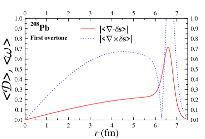
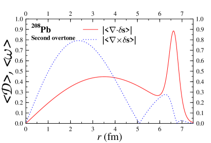
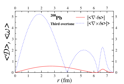
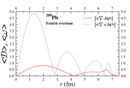
Figure 2: Compresibility and vorticity of the first four overtones of the ISGDR in ²⁰⁸Pb.

The procedure to quantize a continuum system, described by the equation of continuity and the equation of motion (8) is to expand $\delta\rho$ and $\delta\mbox{\boldmath$s$}$ in normal coordinates feenberg69 :

$$\delta\rho(\mbox{\boldmath$r$},t)=\sum_{n}{\cal\rho}_{n}(\mbox{\boldmath$r$})\alpha_{n}(t),~{}~{}~{}~{}~{}\delta\mbox{\boldmath$s$}(\mbox{\boldmath$r$},t)=\sum_{n}\mbox{\boldmath$s$}_{n}(\mbox{\boldmath$r$})\alpha_{n}(t)$$ (18)

The above sums are running after the values of $k_{L}(k_{T})$ allowed by the boundary condition (17), i.e. after the overtones $n$. For the expression of the kinetic energy in the newly introduced collective coordinates $\alpha_{n}$ we have

$$T=\frac{1}{2}\rho_{0}\int~{}d\mbox{\boldmath$r$}|\delta\dot{\mbox{\boldmath$s$}}(\mbox{\boldmath$r$},t)|^{2}\equiv\frac{1}{2}\sum_{n}B_{n}|\dot{\alpha}_{n}|^{2}$$ (19)

For the mass inertia parameter we derive the expression

$$B_{n}=\frac{3mA}{4\pi}\left\{\left[\frac{1}{2}\left(j_{0}^{2}(k_{L}^{(n)}R_{0})+j_{1}^{2}(k_{L}^{(n)}R_{0})\right)-\frac{1}{2k_{L}^{(n)}R_{0}}j_{1}(k_{L}^{(n)}R_{0})\left(j_{0}(k_{L}^{(n)}R_{0})+\frac{6}{k_{L}^{(n)}R_{0}}j_{1}(k_{L}^{(n)}R_{0})\right)\right]\right.$$

$$\left.+r_{n}^{2}\left[\frac{1}{2}\left(j_{0}^{2}(k_{T}^{(n)}R_{0})+j_{1}^{2}(k_{T}^{(n)}R_{0})\right)-\frac{1}{2k_{T}^{(n)}R_{0}}j_{1}(k_{T}^{(n)}R_{0})\left(j_{0}(k_{T}^{(n)}R_{0})+\frac{6}{k_{T}^{(n)}R_{0}}j_{1}(k_{T}^{(n)}R_{0})\right)\right]\right\}$$

The stiffness coefficient associated to an oscillation of degree $n$ is simply

$$C_{n}=\Omega_{n}^{2}B_{n}$$

and the quantized form of the energy can be obtained by introducing the creation and annihilation dipole ”gions” gre70

$$\hat{d}_{n}^{+}=\left(\frac{\Omega_{n}B_{n}}{2\hbar}\right)^{\frac{1}{2}}\left(\alpha_{n}-\frac{i}{\Omega_{n}}\dot{\alpha}_{n}\right),~{}~{}~{}~{}~{}~{}\hat{d}_{n}=\left(\frac{\Omega_{n}B_{n}}{2\hbar}\right)^{\frac{1}{2}}\left(\alpha_{n}+\frac{i}{\Omega_{n}}\dot{\alpha}_{n}\right)$$

The collective Hamiltonian will then read

$$\hat{H}=\sum_{n}\hbar\Omega_{n}\left(\hat{d}_{n}^{\dagger}\hat{d}_{n}+\frac{1}{2}\right)$$ (21)

III Electromagnetic structure of ISGDR

III.1 Low-$q$ limit of the form-factors multipole parametrization

To disclose the structure of the ISGDR we adopt the multipolar parametrization of charges and currents according to dubche74 . In this approach the classical electromagnetic multipoles are expanded in the momentum transfer in reactions with photons, electrons or charged hadrons. Let us take first the charge multipole form-factor for the charge part of the ISGDR fluctuation density:

$$M_{\lambda\mu}^{\rm C}(q,t)=\int d\mbox{\boldmath$r$}j_{\lambda}(qr)Y_{\lambda\mu}(\vartheta\varphi)\delta\rho_{p}(\mbox{\boldmath$r$},t)\approx\frac{q^{\lambda}}{(2\lambda+1)}\left(Q_{\lambda\mu}(t)-\frac{1}{2(2\lambda+3)}q^{2}\overline{\varrho_{\lambda\mu}^{2}}(t)\right)$$ (22)

The first terms of the above $q$-expansion represents the transition charge dipole moment

$$Q_{\lambda\mu}(t)=\delta_{\lambda,1}\delta_{\mu,0}\int d\mbox{\boldmath$r$}r^{\lambda}Y_{\lambda\mu}(\theta,\phi)\delta\rho_{p}(\mbox{\boldmath$r$},t)=0,$$ (23)

a quantity which vanishes for the ISGDR due to the constraint imposed on the c.m. motion. For the IVGDR this will not be the case, since the dynamical dipole moment arises naturally as a measure of the relative motion between the ”negative” charge (neutron) distribution and the positive charge (proton) distribution. Instead the next term in the expansion (22), does not cancel. The quantitiy

$$\overline{\varrho_{\lambda\mu}^{2}}(t)=\delta_{\lambda,1}\delta_{\mu,0}\int d\mbox{\boldmath$r$}r^{\lambda+2}Y_{\lambda\mu}(\theta,\phi)\delta\rho_{p}(\mbox{\boldmath$r$},t)=2\rho_{0p}R_{0}^{5}\sum_{n}\alpha_{n}(t)\frac{j_{\lambda}(k_{L}^{(n)}R_{0})}{k_{L}^{(n)}R_{0}}$$ (24)

represents the mean square radius of the dipole charge distribution. It provides informations on the spatial extension of the ISGDR and it depends only on the longitudinal(compressional) part of the displacement field which are related via the continuity equation (2) to the density fluctuations.

According to the charge-current multipole parametrization of dubche74 , the electric transverse form factor, splits into the ${q}=0$ limit and a term containing the higher order content in $q$.

$$T_{\lambda\mu}^{\rm E}(q,t)=\frac{i^{\lambda+1}}{(2\lambda+1)!!}q^{\lambda-1}\sqrt{\frac{\lambda+1}{\lambda}}\left(\dot{Q}_{\lambda\mu}(0,t)+q^{2}T_{\lambda\mu}^{\rm tor}(q,t)\right)$$ (25)

The first term in the paranthesis is the time-derivative of the Coulomb multipole moment defined in eq.(23) The second term represents the toroidal form factor that reads in the low-$q$ limit

$$T_{\lambda\mu}^{\rm tor}(0,t) = -\frac{1}{2}\sqrt{\frac{\lambda}{2\lambda+1}}\int d\mbox{\boldmath$r$}~{}r^{\lambda+1}\left[\mbox{\boldmath$Y$}_{\lambda\lambda-1}^{\mu}+\frac{2}{2\lambda+3}\sqrt{\frac{\lambda}{\lambda+1}}\mbox{\boldmath$Y$}_{\lambda\lambda+1}^{\mu}\right]\cdot\mbox{\boldmath$j$}(\mbox{\boldmath$r$},t)$$ (26)

$$= \frac{1}{2i}\sqrt{\frac{\lambda}{\lambda+1}}\frac{1}{2\lambda+3}\int d\mbox{\boldmath$r$}~{}r^{\lambda+2}\mbox{\boldmath$Y$}_{\lambda\lambda}^{\mu}\cdot(\nabla\times\mbox{\boldmath$j$}(\mbox{\boldmath$r$},t))$$ (27)

In classical electrodynamics the transition toroidal multipole moment is associated to a poloidal flow on the wings of a toroidal solenoid (for details see the reviews dubche74 ). In the study of electric collective states it can be related to the strength of the vorticity associated to a nuclear transition. Indeed, following ref.ravwam87 , we introduce the transition multipoles of the curl of the current density (unconstrained by the charge-current conservation law)

$${\cal T}_{\lambda\lambda}(r)\equiv\langle I_{f}\parallel(\nabla\times\mbox{\boldmath$j$}(\mbox{\boldmath$r$},t))_{\lambda\lambda}\parallel I_{i}\rangle$$

In order to remove the charge-current conservation constraint, the authors of ravwam87 introduced the pure vorticity transition multipole

$$\omega_{\lambda\lambda}={\cal T}_{\lambda\lambda^{\prime}}(r)-\sqrt{\frac{\lambda+1}{\lambda}}\Omega\rho_{\lambda}$$ (28)

where $\rho_{\lambda}$ is the charge density multipole and $\Omega$ the energy associated to the transition. If the quantity

$$\nu_{\lambda}=\int_{0}^{\infty}dr~{}r^{\lambda+4}\omega_{\lambda\lambda}(r)$$

is defined according to ravwam87 as the strength of the vorticity and employing the definitions (24) for the square of the dynamic dipole charge distribution and (27) for the dynamic dipole toroidal moment we arrive at the expression relating the r.m.e. of these last two electromagnetic multipoles and the vorticity strength

$$\langle I_{f}=1_{n}^{-}\parallel T_{1}^{\rm tor}\parallel I_{i}=0\rangle=\frac{i}{10}\left[\frac{1}{\sqrt{2}}\nu_{1}+\Omega_{n}\langle I_{f}=1_{n}^{-}\parallel\overline{\varrho_{1}^{2}}\parallel I_{i}=0\rangle\right]$$ (29)

From this last formula we see that since the toroidal dipole moment and the square radius of the dipole charge distribution are the leading terms in the $q$-expansion of the transverse electric (25) and Coulomb (22) form factors for the ISGDR, the determination of these two electromagnetic multipoles at low $q$ allows the determination of the vorticity content unconstrained by the charge-current conservation law. Before ending this section we give the classical expression of the transition toroidal dipole moment associated to the ISGDR. Since the current density reads in this case

$$\mbox{\boldmath$j$}=e\frac{Z}{A}n_{0}\sum_{n=1}\left(\delta\mbox{\boldmath$s$}_{L}^{(n)}(\mbox{\boldmath$r$})+r_{n}\delta\mbox{\boldmath$s$}_{T}^{(n)}(\mbox{\boldmath$r$})\right)$$ (30)

we finally obtain

$$T_{1}^{\rm tor}(0,t)={\frac{1}{10\sqrt{2}}}\rho_{0p}R_{0}^{5}\sum_{n}r_{n}\dot{\alpha}_{n}(t)\frac{j_{3}(k_{T}^{(n)}R_{0})}{k_{T}^{(n)}R_{0}}$$ (31)

Thus, the dipole toroidal moment depends only on the shear(vortical) part of the proton fluid displacement field.

III.2 Electro-excitation form factors of ISGDR

Inelastic electron scattering is an excellent tool to explore the nature of currents involved in the excitation of low-lying (rotational or vibrational) and high-lying (giant resonances) collective states ueberall . A specific feature of this reaction is represented by the possibility to separate the longitudinal from the transverse response functions. This is of vital importance if one tries to disentangle the compresional from the vortical response in the excitation of a specific electric collective state.

III.3 (e,e^′) form factors

Quantizing the expression of the fluctuation density (15) and inserting it in the square of the reduced matrix element(r.m.e.) of the Coulomb multipole operator (22) leads to

$$\mid\langle I_{f}=1^{-}\parallel{\hat{M}}_{\lambda}^{\rm C}\parallel I_{i}=0\rangle|^{2}=3\left[\rho_{0p}R_{0}^{2}\sum_{n}F_{\rm C}^{(n)}(q)\right]^{2}$$ (32)

where

$$F_{C}^{(n)}(q)=\alpha_{n0}\left\{\frac{k_{l}^{(n)}}{q^{2}-{k_{l}^{(n)}}^{2}}\left[k_{l}^{(n)}j_{0}(k_{l}^{n}R_{0})j_{1}(qR_{0})-qj_{0}(qR_{0})j_{1}(k_{l}^{(n)}R_{0})\right]-j_{2}(k_{l}^{(n)}R_{0})j_{1}(qR_{0})\right\}\\$$ (33)

and the amplitude of the canonical coordinate $\alpha_{n}$ is given by the transition r.m.e. of the normal coordinate

$$\alpha_{n0}\equiv\langle I_{f}=1^{-}\parallel{\alpha}_{n}\parallel I_{i}=0\rangle=\left(\frac{\hbar}{2B_{n}\Omega_{n}}\right)^{1/2}$$ (34)

It can be noticed from the content of (33) that not only its low-$q$ limit depend on the longitudinal components of the collective flow ($\delta\mbox{\boldmath$s$}_{L}$), as substantietad by eq.(24), but also its higher order $q$ content. Therefore, the Coulomb form-factor provides solely informations on the compresional waves associated to the ISGDR.

In fig.3 we draw the dependence of (32) on the momentum transfer $q$ for the first four overtones in ²⁰⁸Pb. The diffraction maxima, although shifted to higher values $q$ for increasing overtone number, are not affected in absolute value.

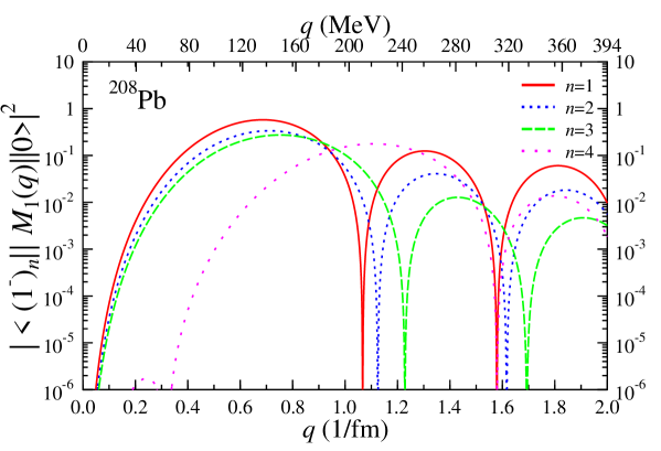
Figure 3: R.m.e. of the Coulomb multipole operator for the first 4 overtones of the ISGDR in ²⁰⁸Pb.

The expression of the squared r.m.e. of the transverse electric operator (25) reduces to

$$\mid\langle I_{f}=1^{-}\parallel\widehat{T}^{\rm E}_{\lambda}(q)\parallel I_{i}=0\rangle|^{2}=3\left[\rho_{0p}R_{0}^{3}\sum_{n}F_{\rm T}^{(n)}(q)\right]^{2}$$ (35)

where

$$F_{T}^{(n)}(q)=r_{n}\Omega_{n}\alpha_{n0}\left\{R_{0}\frac{k_{T}^{(n)}j_{1}(k_{T}^{n}R_{0})j_{0}(qR_{0})-qj_{1}(qR_{0})j_{0}(k_{T}^{(n)}R_{0})}{q^{2}-{k_{T}^{(n)}}^{2}}-\frac{3}{qk_{T}^{(n)}}j_{1}(k_{T}^{(n)}R_{0})j_{1}(qR_{0})\right\}$$ (36)

Thus, contrary to the Coulomb multipoles, the transverse multipoles are providing informations only on the vortical components of the ISGDR. The squared r.m.e. of (35) is ploted in Fig.4. The first diffraction bump dominates for the $n=$1 and 2 components of the ISGDR, whereas for $n$=3 the second bump and for $n=4$ the third bump are taking over. According to Table 1, were we listed the ratio $b_{n}/a_{n}$(vorticity/compressibility), this feature, is a consequence of the vorticity enhancement, in this higher lying states. Instead the first Coulomb diffraction bump maintains its importance in the electro-excitation of higher-lying states because the role played by the density waves is less important for these states.

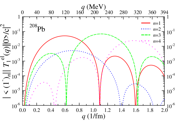
Figure 4: R.m.e. of the transverse multipole operator for the first 4 overtones of the ISGDR in ²⁰⁸Pb.

III.4 Sum rules for electron scattering

It is known that for the isoscalar electric modes simulated by operators depending only on coordinates of the particles the energy-weighted sum rules can be determined model independently and depend only on the ground-state properties of the nucleus boh75 ; deal73 ; har81 ; lipstr89 . Operators from this class are commuting with interactions not depending explicitely on the momenta of the particles. These scalar operators are simulating shape or density distortions corresponding to a given isoscalar multipolar resonance and for that reason in the literature the macroscopic images associated to these excitations are always irrotational surface or bulk compressional oscillations. Instead they are inadequate to describe distortions of the nuclear current which are not constrained by the charge-current conservation law, i.e. excitations with vortical currents. A class of sum-rules coping with both kind of distortions, i.e. of charge density and current (unconstrained by the charge-current relations) is given by the longitudinal ($L$) and transverse ($T$) intrinsic energy weighted sum-rules (EWSR) at constant three-momentum transfer $|\mbox{\boldmath$q$}|$, which are constructed by weighting the nuclear response functions torn80

$$R^{L}(\mbox{\boldmath$q$},E^{*}) = \sum_{n}^{\infty}\mid\langle n\mid\rho(\mbox{\boldmath$q$})\mid 0\rangle\mid^{2}\delta\left(E^{*}-\frac{\hbar^{2}q^{2}}{2M_{A}}-E_{n}\right)$$ (37)

$$R^{T}(\mbox{\boldmath$q$},E^{*}) = \sum_{n}^{\infty}\mid\langle n\mid\mbox{\boldmath$J$}_{\bot}(\mbox{\boldmath$q$})\mid 0\rangle\mid^{2}\delta\left(E^{*}-\frac{\hbar^{2}q^{2}}{2M_{A}}-E_{n}\right)$$ (38)

with an appropriate power of the nuclear excitation energy $E^{*}$. Summing over all excited states we obtain the intrinsic $p$-order EWSR depending on $q$

$${m_{p}^{L}}(q) = \int d{E^{*}}^{\prime}R^{L}(\mbox{\boldmath$q$},{E^{*}}^{\prime}){E^{*}}^{p}=\sum_{n}^{\infty}E_{n}^{p}\langle n\mid\rho(\mbox{\boldmath$q$})\mid 0\rangle\mid^{2}$$ (39)

$${m_{p}^{T}}(q) = \int dE^{*\prime}{R^{T}}(\mbox{\boldmath$q$},E^{*\prime}){{E}^{*\prime}}^{p}=\sum_{n}^{\infty}{E_{n}^{p}}\langle n\mid\mbox{\boldmath$J$}_{\bot}(\mbox{\boldmath$q$})\mid 0\rangle\mid^{2}$$ (40)

where $E^{*\prime}={E}^{*}-\hbar^{2}q^{2}/2M_{A}$ is the energy available for intrinsic excitations. In the above formula $\mbox{\boldmath$J$}_{\bot}(\mbox{\boldmath$q$})$ denotes the transverse component of the current operator relative to the momentum transfer$(\mbox{\boldmath$J$}_{\bot}(\mbox{\boldmath$q$})=\mbox{\boldmath$J$}(\mbox{\boldmath$q$})-\mbox{\boldmath$q$}(\mbox{\boldmath$q$}\cdot\mbox{\boldmath$J$})/\mbox{\boldmath$q$}^{2})$.

The longitudinal and transverse $p-$order energy strengths of each state can then be obtained as relative contributions to the corresponding sum-rules (39) and (40)

$$E_{n}^{p}\mid\langle n\mid\rho(\mbox{\boldmath$q$})\mid 0\rangle\mid^{2}/{{m_{p}}^{L}}(q),~{}~{}~{}~{}~{}E_{n}^{p}\mid\langle n\mid\mbox{\boldmath$J$}_{\bot}(\mbox{\boldmath$q$})\mid 0\rangle\mid^{2}/{{m_{p}}^{T}}(q)$$

In Figs.5 and 6 we represent the zeroth- and first- order strengths distributions for the longitudinal and transverse responses. In the sums only the first three overtones were included and therefore the excitation energy is truncated at 30 MeV. We see that for very low momentum transfer the $L$ and $T$ strength is mainly concentrated on the first overtone. When $q$ increases the $L$ and $T$ strengths follow a different pattern. Whilst the $L$ strength is fragmented almost ”democratically” over the three overtones, the $T$ strengths are testifying a transition from a low-$q$ regime where the first overtone dominates to a high-$q$ regime where the third overtone overtakes the predominance. For both regimes the second overtone plays a very minor role. This fact can be explained in our view by the compressibility content of this mode which is ”washed-out” in the transverse response function. In the longitudinal response the second overtone plays a more visible role.

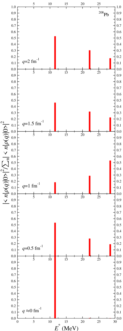
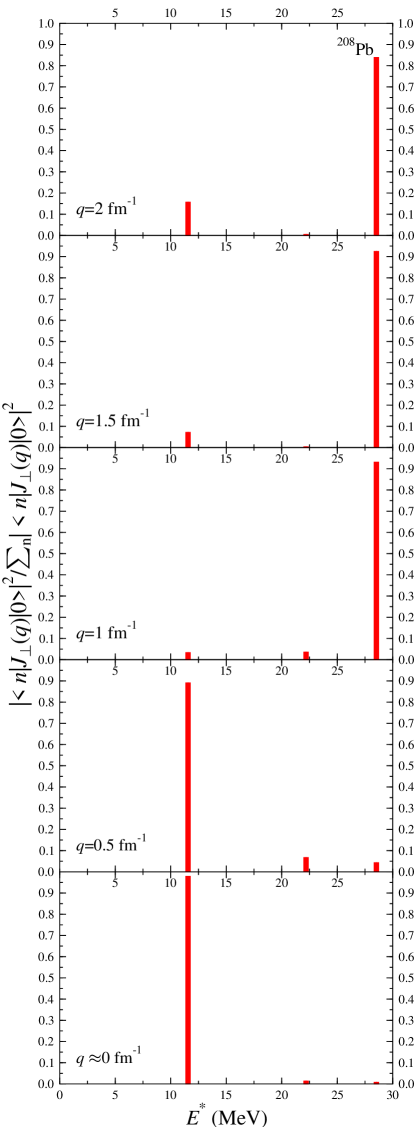
Figure 5: Zeroth-order energy strengths distributions for $\rho$ and $\mbox{\boldmath$J$}_{\perp}$. The energy cut is $(E^{*})_{\rm cut}$ = 30 MeV.

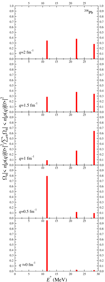
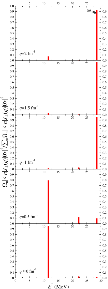
Figure 6: First-order energy strengths distributions for $\rho$ and $\mbox{\boldmath$J$}_{\perp}$. The energy cut is $(E^{*})_{\rm cut}$ = 30 MeV.

In the low-$q$ limit the ratios $m_{1}/m_{0}$ and $\sqrt{m_{3}/m_{1}}$ are expected to provide crude estimates for the mean excitation energies associated to the density or transverse density current distortions. In Table 2 we list these mean excitation energies for a series of spherical nuclei. Comparing the obtained values to the eigenvalues of the first two overtones we notice that the ratio ${m_{1}}^{L}/{m_{0}}^{L}$ gives the best estimate of the first overtone. For the second overtone the ratio $\sqrt{{m_{3}}^{T}/{m_{1}}^{T}}$ gives a rather coarse approximate. The other two ratios are falling in the vicinity of the first overtone.

Nucleus	${m_{1}}^{L}/{m_{0}}^{L}$	$\sqrt{{m_{3}}^{L}/{m_{1}}^{L}}$	${m_{1}}^{T}/{m_{0}}^{T}$	$\sqrt{{m_{3}}^{T}/{m_{1}}^{T}}$	$\hbar\Omega_{1}$	$\hbar\Omega_{2}$	$(\hbar\Omega_{1})_{\rm exp}$	$(\hbar\Omega_{2})_{\rm exp}$
	(MeV)	(MeV)	(MeV)	(MeV)	(MeV)	(MeV)	(MeV)	(MeV)
90Zr	15.44	16.29	16.86	25.53	15.28	29.34	16.20$\pm$0.80	25.70$\pm$0.701)
116Sn	14.19	14.99	15.51	23.68	14.04	26.96	14.38$\pm$0.25	25.50$\pm$0.601)
							14.70$\pm$0.80	23.00$\pm$0.602)
144Sm	13.21	14.07	14.64	23.95	13.07	25.08	14.00$\pm$0.30	24.51$\pm$0.401)
208Pb	11.68	12.44	12.96	21.19	11.56	22.19	13.26$\pm$0.30	22.20$\pm$0.301)
							12.50$\pm$0.30	22.50$\pm$0.302)

Table 2: Ratios of ISGDR sum rules for $q\longrightarrow 0$ compared to the energies of the first two overtones for ⁹⁰Zr, ¹¹⁶Sn, ¹⁴⁴Sm and ²⁰⁸Pb and with experimental latest experimental data from young04 ¹⁾ and uch03 ²⁾ for the low- and high-energy peaks .

IV Summary and Conclusion

The lower and upper component of the ISGDR, as reported by the latest experimental measurements, are explained as the first two overtones of a spherical Fermi-Fluid system with a sharp free surface corresponding to a mixture of dipole compression and vorticity oscillations.

The approach presented in this work was applied primary to the heavy spherical nucleus ²⁰⁸Pb, because in this case the sharp-edge density distribution assumption is more acceptable as would be the case for lighter nuclei for which experimental data on ISGDR are available (⁴⁰Ca, ⁹⁰Zr, ¹¹⁶Sn and ¹⁴⁴Sm) and where the diffuse surface plays an important role. In order to extend the analysis of ISGDR to these nuclei and also to exotic nuclei that are presently under intense investigations, one should adopt at first a more realistic assumption for the ground-state density distribution. In this case along with the density, other parameters of the nuclear Fermi liquid. e.g. the Lamé coefficients acquire a radial dependence and the equations of motions must be solved numerically.

In the present approach, the excitation of the ISGDR is not limited to the squeezing operator. It includes the entire momentum content in the operator $j_{1}(kr)Y_{1}({\hat{r}})$ and takes into account also its c.m. correction via constraints on the density and displacement field fluctuations. Moreover, since there is no mathematical or physical exception it considers along with the longitudinal solution also the transverse solution of the vector Helmholz equation. Conseqently the overtones of the ISGDR are mixtures of compressional and vortical velocity fields. For the second overtone, previously advocated to be of compressional nature, the nuclear Fermi-Fluid approach confirms very recent microscopical predictions cro-ring01 ; kvasil03 that are pointing toward a cohabitation of compressional and vorticity vibrations in the ISGDR states up to 30 MeV.

Naturally, a question arise : Has been gained so far any indication in experiment on the overtones with $n\geq 3$, located above the ”high-lying” ISGDR state? For the time being this question cannot be answered because the latest data reported by the College Station group young04 are providing very large uncertainties in the strength distribution for ²⁰⁸Pb beyond the second peak, i.e. at excitation energy $>3\hbar\omega$.

A study of the electromagnetic multipole transitions was undertaken and concluded that the leading term in the Coulomb form-factor is singled-out only by the density fluctuation and can be related to the rms-charge radii. In turn the leading mutipole in the transverse electric form factor, the toroidal dipole moment, results soleley from the transverse part of the velocity field. In this respect the r.m.e. of the toroidal dipole transition provide a signature of vorticity through electromagnetic probes.

The $(e,e^{\prime})$ are promising candidates for the exploration of the role of longitudinal and vortical currents of ISGDR since the separation of longitudinal (Coulomb) and electric transverse form-factor is feasible. However in such reactions it is difficult to avoid the excitation of the dominant electric dipole response, the IVGDR. It would be in this respect interesting to search for a macroscopical description that deals in a unified manner with the isoscalar and isovector electric dipole responses.

Appendix A Scalar and vector Helmholz equations

The solution of the scalar HE (10) reads

$${\cal D}=\sum_{\lambda\mu}a_{\lambda\mu}j_{\lambda}(k_{L}r)Y_{\lambda\mu}(\theta,\phi)$$ (41)

The solution of the vector HE splits into an electric(poloidal) and a magnetic(torsional) solution

$$\mbox{\boldmath$\omega$}^{\rm pol} = \sum_{\lambda\mu}b_{\lambda\mu}^{\rm el}j_{\lambda}(k_{T}r)\mbox{\boldmath$Y$}_{\lambda\lambda}^{\mu}(\theta,\phi)$$ (42)

$$\mbox{\boldmath$\omega$}^{\rm tor} = \sum_{\lambda\mu}b_{\lambda\mu}^{\rm el}\frac{1}{\sqrt{2\lambda+1}}\left(\delta_{\lambda^{\prime}\lambda-1}\sqrt{\lambda+1}-\delta_{\lambda^{\prime}\lambda+1}\sqrt{\lambda}\right)j_{\lambda^{\prime}}(k_{T}r)\mbox{\boldmath$Y$}_{\lambda\lambda^{\prime}}^{\mu}(\theta,\phi)$$ (43)

In the present study on electric resonances we are interested only in the poloidal solution. Using the properties of the spherical harmonic vectors we can derive the expression of the longitudinal and transverse displacements fields. Since $\delta\mbox{\boldmath$s$}_{L}$ results from the definition of the scalar function

$${\cal D}\equiv\nabla\cdot\delta\mbox{\boldmath$s$}=\nabla\cdot\delta\mbox{\boldmath$s$}_{L}$$ (44)

we have that

$$\delta\mbox{\boldmath$s$}_{L}=-\frac{1}{k_{L}}\sum_{\lambda\mu}a_{\lambda\mu}\frac{1}{\sqrt{2\lambda+1}}\left(\delta_{\lambda^{\prime}\lambda-1}\sqrt{\lambda^{\prime}+1}+\delta_{\lambda^{\prime}\lambda+1}\sqrt{\lambda^{\prime}}\right)j_{\lambda^{\prime}}(k_{L}r)\mbox{\boldmath$Y$}_{\lambda\lambda^{\prime}}^{\mu}(\theta,\phi)$$ (45)

Similarly, from the definition of the vorticity

$$\mbox{\boldmath$\omega$}^{\rm pol}\equiv\frac{1}{2}\nabla\times\delta\mbox{\boldmath$s$}_{T}$$ (46)

we get

$$\delta\mbox{\boldmath$s$}_{T}=\frac{i}{k_{T}}\sum_{\lambda\mu}b_{\lambda\mu}\frac{1}{\sqrt{2\lambda+1}}\left(\delta_{\lambda^{\prime}\lambda+1}\sqrt{\lambda^{\prime}}-\delta_{\lambda^{\prime}\lambda+1}\sqrt{\lambda^{\prime}-1}\right)j_{\lambda^{\prime}}(k_{T}r)\mbox{\boldmath$Y$}_{\lambda\lambda^{\prime}}^{\mu}(\theta,\phi)$$ (47)

References

- (1) H.L.Clark, Y.-W.Lui and H.Youngblood, Phys.Rev.C63, 031301(R) (2001).
- (2) H.Youngblood, Y.-W.Lui, B.John, Y.Tokimoto, H.L.Clark and X.Chen,Phys.Rev.C69, 054312 (2004).
- (3) M. Uchida et al., Phys.Lett.B557, 12 (2003).
- (4) H.P.Morsch et al.,Phys.Rev.C28, 1947 (1983).
- (5) J.J. Deal, Nucl.Phys.A 217, 210(1973).
- (6) M.N. Harakeh and A.E.L. Dieperink, Phys.Rev.C23, 2329 (1981).
- (7) J. Wambach, V.Klemt and J.Speth, Phys.Lett.B77, 245 (1978).
- (8) N. Van Giai and H. Sagawa, Nucl.Phys.A371, 1 (1981).
- (9) I. Hamamoto, H. Sagawa and X.Z. Zhang, Phys.Rev.C57, R1064 (1998).
- (10) T.S. Dumitrescu and F.E.Serr, Phys.Rev.C27, 811 (1983).
- (11) G. Coló, N. Van Giai, P.F. Bortignon and M.R. Quaglia, Phys.Lett.B485, 362 (2000).
- (12) S. Shlomo and A.I. Sanzhur, Phys.Rev.C65, 044310 (2002).
- (13) M.L. Gorelik,I.V. Safonov and M.H. Urin, Phys.Rev.C69, 054322 (2004).
- (14) D. Vretenar, A. Wandelt and P. Ring, Phys.Lett.B487, 334 (2000).
- (15) K. Woeste, Zeit.für Physik, 133, 370 (1952).
-
(16)
V.M.Kolomietz and S.Shlomo, Phys.Rev.C61,
064302, (2000)
V.M.Kolomietz and S.Shlomo, Phys.Rep.390, 133 (2004). - (17) G.Holzwarth and G.Eckardt, Nucl.Phys.A325, 1 (1979).
- (18) S.F. Semenko, Yad.Fiz.34, 639 (1981) [engl.transl.Sov.J.Nucl.Phys.34, 356(1981)].
-
(19)
V.M. Dubovik and A.A. Cheshkov, Fiz.Elem.Chastits At. Yadra
5, 792 (1974)[engl.transl. Sov.J.Part.Nucl5, 318 (1975).].
V.M. Dubovik and V.V. Tugushev, Phys.Rep.187, no.4, 145 (1990). - (20) E.B. Balbutsev and I.N.Mikhailov, J.Phys.G 14, 545 (1988).
- (21) S.I. Bastrukov, Ş.Mişicu and V.I.Sushkov, Nucl.Phys.A562, 191 (1993).
- (22) Ş. Mişicu, Dissertation, Institute for Atomic Physics (1995)(in romanian) [abridged version in engl.transl. : Ş.Mişicu, Rom.J.Phys.43, 193 (1998)].
- (23) Ş. Mişicu, J.Phys.G:Nucl.& Part.Phys.21, 669 (1995).
- (24) I.N. Mikhailov, Ch.Briançon and P.Quentin, Fiz.Elem.Chastits i At.Yadra 27, 303 (1996).
- (25) D. Vretenar, N. Paar, P. Ring and T. Niks̆ić, Phys.Rev.C65, 021301 (2001).
- (26) Ş. Mişicu and S.I.Bastrukov, Eur.Phys.J. A 13, 399 (2002).
- (27) N.Ryezayeva et al., Phys.Rev.Lett.89, 272502-1 (2002).
- (28) J. Kvasil, N.Lo Iudice, Ch.Stoyanov and P.Alexa, J.Phys.G:Nucl.& Part.Phys.29, 753 (2003).
- (29) C.-Y. Wong and N. Azziz, Phys.Rev.C 24, 2290 (1981).
- (30) Arnold Sommerfeld, Mechanik der deformierbaren Medien, Verlag Harri Deutsch, Frankfurt am Main, 1978 (english translation Mechanics of Deformable Bodies, New York, Academic Press, 1950).
- (31) J.P.Blaizot, Phys.Rep.64, no.4, 171 (1980).
- (32) Ari Ben-Menahem and Sarva Jit Singh, Seismic Waves and Sources, Springer-Verlag, New York Inc., 1981.
- (33) P.M. Morse and H. Feschbach, Methods of Theoretical Physics, Part I, Mc Graw-Hill, Part II, 1953.
- (34) S.I.Bastrukov, J.Libert and I.V.Molotsova, Int.J.Mod.Phys.E6, 89 (1997).
- (35) J.Eisenberg and W.Greiner, Nuclear Models, vol.I, North-Holland, Amsterdam, 1970.
- (36) G. Eckart, G. Holzwarth, and J.P. da Providencia, Nucl.Phys.A364, 1 (1981)
- (37) A. Bohr and B.R. Mottelson, Nuclear Structure, vol.II, W.A.Benjamin Inc., Amsterdam 1974.
-
(38)
F.E. Serr, T.S. Dumitrescu, T.Suzuki and C.H.Dasso,
Nucl.Phys.A404 , 359 (1983).
T.S. Dumitrescu, C.H. Dasso, F.E. Serr and T.Suzuki, J.Phys.G12, 349 (1986). - (39) E. Feenberg, Theory of Quantum Fluids, Academic Press, New York & London 1969.
- (40) D.G. Ravenhall and J. Wambach, Nucl.Phys.A475, 468 (1987).
- (41) H.Überall, Electron Scattering from Complex nuclei, part A, Academic Press, New York and London, 1971.
- (42) E. Lipparini and S. Stringari, Phys.Rep.175, 103 (1989).
- (43) V.Tornow et al., Nucl.Phys. A348, 157 (1980).