Study of Resonant Structures in a Deformed Mean-Field by the Contour Deformation Method in Momentum Space.

Abstract

Solution of the momentum space Schrödinger equation in the case of deformed fields is being addressed. In particular it is shown that a complete set of single particle states which includes bound, resonant and complex continuum states may be obtained by the Contour Deformation Method. This generalized basis in the complex energy plane is known as a Berggren basis. The momentum space Schrödinger equation is an integral equation which is easily solved by matrix diagonalization routines even for the case of deformed fields. The method is demonstrated for axial symmetry and a fictitious ”deformed ⁵He”, but may be extended to more general deformation and applied to truly deformed halo nuclei.

I Introduction

In nuclear physics, like in atomic physics, expansion of many-body wavefunctions on single particle bases, generated by a suitable potential has been common practice. The newly developed Gamow Shell Model Michel et al. (2004a, b); Dobaczewski et al. (2004); Michel et al. (2002, 2003); IdBetan et al. (2002, 2003, 2004); Hagen et al. (2004, 2005) starts with the Berggren completeness Berggren (1968, 1971, 1978, 1996); Lind (1993). The Gamow Shell Model has proven to be a promising tool in assessing the structure of weakly bound and unbound nuclei. The Berggren completeness is a generalized completeness which treats bound and resonant states on equal footing. The completeness is given by a discrete sum over bound and resonant states and accomponied by an integral over a non-resonant continuum of scattering states with complex energy. A complete many-body Berggren basis may then be constructed from discretized single-particle Berggren orbitals where many body Slater determinants are constructed from the discrete bound, resonant and non-resonant continuum orbitals. This is the philosophy of the Gamow Shell Model in full analogy with the standard Shell Model using a harmonic oscillator basis.

In this paper we address the problem of how to accurately calculate for resonances in deformed fields. Further, it is discussed how to obtain a complete set of states suitable for use in scattering/reaction problems, where spectral representations of Green’s functions are of great interest, and in other many-body applications. The study of resonances in deformed fields has so far only rarely been considered, and for special cases. In Ref. Kruppa et al. (2004) the solution of the angular momentum coupled Schrödinger equation was considered for a deformed Woods-Saxon. They diagonalized the deformed Hamiltonian using a Berggren basis generated from the spherical Woods-Saxon potential in position space, and compared with other methods such as an expansion in oscillator functions and a direct solution of the coupled equations. In Ref. Ferreira et al. (1997) energy levels and conditions for bound states to become resonances and resonances to become bound states were investigated for an axially deformed Woods-Saxon potential, by solving the the radial Schrödinger equation for coupled channels with outgoing asymptotics. However, the coupled channels method used in Ref. Ferreira et al. (1997) does not easily generalize to the non-resonant continuum. This implies that a complete Berggren basis in a deformed field is difficult to obtain, and all evaluated observables will become complex quantities unless the non-resonant continuum is taken properly into account. In Ref. Hagino and Giai (2004) a different approach was considered. Their aim was to propose a method to obtain scattering wave functions in the vicinity of a multi-channel resonance on the real axis, then calculate the phase shifts, and investigate whether a resonance condition is met. Further this method allows for evaluation of observables where the continuum is properly taken into account, and the observables become real quantities.

In this paper we propose an alternative method, starting with the momentum space Schrödinger equation given in Eq. (1). In Ref. Hagen et al. (2004) it was shown how a complete set of Berggren states may be obtained by an analytically continuation of the momentum space Schrödinger equation in the complex $k$-plane by utilizing the Contour-Deformation-Method (CDM). By a suitable choice of deformed integration contour $L^{+}$ we demonstrated that all physical resonances converges extremely fast with respect to number of integration points. Further it was shown that for a particular type of contour $L^{+}$, stable solutions of all physical scattering amplitudes may be obtained by a spectral representation of the Green’s function. The main difference between a momentum space approach and a position space approach (see e.g. Ref. Kruppa et al. (2004)), lies in their different discretization schemes. In momentum space, it is the Bessel completeness which is discretized, while in position space it is the completeness of the one-body problem (for example a Woods-Saxon completeness) which is discretized. The obvious advantage of the momentum space approach lies in its immediate simplicity. Firstly, the boundary conditions are automatically built into the integral equations. Secondly, the discretized Schrödinger equation is a complex symmetric matrix which is easily diagonalized, and last but not least convergence is obtained by increasing the number of integration points.

In sec. II the 1-dimensional angular momentum coupled integral equations in momentum space are derived. Sec. III briefly discusses how the integral equations may be analytically continued in the complex $k$-plane by CDM, and the relevant equations for numerical implementations are given. In Sec. IV a deformed field of Gaussian type is introduced, and a brief study of different axially symmetric deformations and multipoles is given. Sec. V derives the multipole components of the Gaussian potential in momentum space. Sec. VI gives results for single-particle resonances in the deformed Gaussian potential, and finally conclusions are given in Sec. VII.

II Momentum Space Representation of the Schrödinger Equation.

The momentum space single-particle Schödinger equation is given by,

$${\hbar^{2}\over 2\mu}k^{2}\psi_{n}({\bf k})+\int d{\bf k^{\prime}}\>V({\bf k},{\bf k^{\prime}})\psi_{n}({\bf k^{\prime}})=E_{n}\psi_{n}({\bf k}).$$ (1)

Here the notation $\psi_{n}({\bf k})=\langle{\bf k}|\psi_{n}\rangle$ and $\langle{\bf k}|V|{\bf k}^{\prime}\rangle=V({\bf k},{\bf k^{\prime}})$ has been introduced. The potential in momentum space is thus a double Fourier-transform of the potential in coordinate space, i.e.

$$V({\bf k},{\bf k^{\prime}})=\left({1\over 2\pi}\right)^{3}\int\mathrm{d}{\bf r}\int\mathrm{d}{\bf r}^{\prime}\>e^{-i{\bf k\cdot r}}V({\bf r},{\bf r}^{\prime})e^{i{\bf k}^{\prime}\cdot{\bf r}^{\prime}}.$$ (2)

Here it is assumed that the interaction potential does not contain any spin dependence. Instead of an differential equation in coordinate space (integro-differential equation for non-local potentials), the Schrödinger equation has become an integral equation in momentum space. This has many tractable features. Firstly, most realistic nucleon-nucleon interactions derived from field-theory are given explicitly in momentum space. Secondly, the boundary conditions imposed on the differential equation in coordinate space are automatically built into the integral equation. And last, but not least, integral equations are easy to numerically implement, and convergence is obtained by just increasing the number of integration points. Instead of solving the three-dimensional integral equation given in Eq. (1), an infinite set of 1-dimensional equations can be obtained by invoking a partial wave expansion. To this end the wave function $\psi_{n}({\bf k})$ is expanded in a complete set of spherical harmonics, i.e.

$$\psi_{n}({\bf k})=\sum_{lm}\psi_{nlm}(k)Y_{lm}(\hat{k}),\>\>\psi_{nlm}(k)=\int d\hat{k}Y_{lm}^{*}(\hat{k})\psi_{n}({\bf k}).$$ (3)

By inserting Eq. 3 in Eq. (1), and projecting $Y_{lm}(\hat{k})$ from the left, the three-dimensional Schrödinger Eq. (1) is reduced to an infinite set of 1-dimensional angular momentum coupled integral equations,

$$\left({\hbar^{2}\over 2\mu}k^{2}-E_{nlm}\right)\psi_{nlm}(k)=-\sum_{l^{\prime}m^{\prime}}\int_{0}^{\infty}dk^{\prime}{k^{\prime}}^{2}V_{lm,l^{\prime}m^{\prime}}(k,k^{\prime})\psi_{nl^{\prime}m^{\prime}}(k^{\prime}),$$ (4)

where the angular momentum projected potential takes the form,

$$V_{lm,l^{\prime}m^{\prime}}(k,k^{\prime})=\int\mathrm{d}{\hat{k}}\int\mathrm{d}{\hat{k}^{\prime}}\>Y_{lm}^{*}(\hat{k})V({\bf k},{\bf k^{\prime}})Y_{l^{\prime}m^{\prime}}(\hat{k}^{\prime}).$$ (5)

Here $\mathrm{d}{\hat{k}}=\mathrm{d}\theta\sin\theta\>\mathrm{d}\varphi$. In many cases the potential is given in position space, so it is convienient to establish the connection between $V_{lm,l^{\prime}m^{\prime}}(k,k^{\prime})$ and $V_{lm,l^{\prime}m^{\prime}}(r,r^{\prime})$. Inserting position space completeness in Eq. (5) gives

$$V_{lm,l^{\prime}m^{\prime}}(k,k^{\prime})=\int\mathrm{d}{\bf{r}}\int\mathrm{d}{\bf{r}^{\prime}}\>\int\mathrm{d}{\hat{k}}\int\mathrm{d}{\hat{k}^{\prime}}\>Y_{lm}^{*}(\hat{k})\langle{\bf k}|{\bf r}\rangle\langle{\bf r}|V|{\bf r}^{\prime}\rangle\langle{\bf r^{\prime}}|{\bf k}^{\prime}\rangle Y_{lm}(\hat{k}^{\prime})=$$

$$\int\mathrm{d}{\bf{r}}\int\mathrm{d}{\bf{r}^{\prime}}\>\left\{\int\mathrm{d}{\hat{k}}Y_{lm}^{*}(\hat{k})\langle{\bf k}|{\bf r}\rangle\right\}\langle{\bf r}|V|{\bf r}^{\prime}\rangle\left\{\int\mathrm{d}{\hat{k}^{\prime}}\>Y_{lm}(\hat{k}^{\prime})\langle{\bf r^{\prime}}|{\bf k}^{\prime}\rangle\right\}.$$ (6)

Since the plane waves depend only on the absolute values of position and momentum, $|{\bf k}|,|{\bf r}|$, and the angle between them, $\theta_{kr}$, they may be expanded in terms of bipolar harmonics of zero rank Biedenharn and Dam (1965), i.e.

$$e^{i{\bf k}\cdot{\bf r}}=4\pi\sum_{l=0}^{\infty}i^{l}j_{l}(kr)\left(Y_{l}(\hat{k})\cdot Y_{l}(\hat{r})\right)=\sum_{l=0}^{\infty}(2l+1)i^{l}j_{l}(kr)P_{l}(\cos\theta_{kr}).$$ (7)

The addition theorem for spherical harmonics has been used in order to write the expansion in terms of Legendre polynomials. The spherical Bessel functions, $j_{l}(z)$, are given in terms of Bessel functions of the first kind with half integer orders Gradshteyn and Ryzhik (1963); Abramowitz and Stegun (1972),

$$j_{l}(z)=\sqrt{\pi\over 2z}J_{l+1/2}(z).$$

Inserting the plane-wave expansion into the brackets of Eq. (6) yields,

$$\int\mathrm{d}{\hat{k}}Y_{lm}^{*}(\hat{k})\langle{\bf k}|{\bf r}\rangle = \left({1\over 2\pi}\right)^{3/2}4\pi i^{-l}j_{l}(kr)Y_{lm}^{*}(\hat{r}),$$

$$\int\mathrm{d}{\hat{k}^{\prime}}\>Y_{lm}(\hat{k}^{\prime})\langle{\bf r^{\prime}}|{\bf k}^{\prime}\rangle = \left({1\over 2\pi}\right)^{3/2}4\pi i^{l^{\prime}}j_{l^{\prime}}(k^{\prime}r^{\prime})Y_{l^{\prime}m^{\prime}}(\hat{r}).$$

The connection between the momentum- and position space angular momentum projected potentials is then given by,

$$V_{lm,l^{\prime}m^{\prime}}(k,k^{\prime})={2\over\pi}i^{l^{\prime}-l}\int_{0}^{\infty}dr\>r^{2}\int_{0}^{\infty}dr^{\prime}\>{r^{\prime}}^{2}j_{l}(kr)V_{lm,l^{\prime}m^{\prime}}(r,r^{\prime})j_{l^{\prime}}(k^{\prime}r^{\prime}),$$ (8)

which is known as a double Fourier-Bessel transform. The position space angular momentum projected potential is given by,

$$V_{lm,l^{\prime}m^{\prime}}(r,r^{\prime})=\int\mathrm{d}{\hat{r}}\int\mathrm{d}{\hat{r}^{\prime}}\>Y_{lm}^{*}(\hat{r})V({\bf r},{\bf r^{\prime}})Y_{l^{\prime}m^{\prime}}(\hat{r}^{\prime}).$$ (9)

No assumptions of locality/non-locality or deformation of the interaction has so far been made, and the result in Eq. (8) is general. In position space the Schrödinger equation takes form of an integro-differential equation in case of a non-local interaction. In momentum space the Schrödinger equation is an ordinary integral equation of the Fredholm type, see Eq. (4). This is a further advantage of the momentum space approach as compared to the standard position space approach.

III Analytic Continuation of the Momentum Space Schrödinger Equation by CDM.

In Ref. Hagen et al. (2004) we discussed and outlined a method which analytically continues the momentum space Schrödinger equation through the unitarity cut onto the second Riemann sheet of the complex energy plane. The method is based on deforming the integration contour and is known as the contour deformation (distortion) method (CDM). As shown in Refs Hagen et al. (2004, 2005), CDM allows for accurate calculation of a complete set of single-particle states, involving all kinds of poles of the scattering matrix. However, in Refs. Hagen et al. (2004, 2005) only spherically symmetric fields were considered. Here we wish to generalize the method to deformed fields, and therefore we write down the relevant equations for the most general case. The rules for analytic continuation of integral equation with general integral kernels are not outlined here, since they are the same as for spherically symmetric fields. We refer the reader to Ref. Hagen et al. (2004) for further details on analytically continuation of integral equations and CDM.

The 1-dimensional coupled integral equations given in Eq. (4) are analytically continued from the physical to the non-physical energy sheet by distorting the integration contour. Choosing a suitable inversion symmetric contour $L^{+}$, as discussed in Ref. Hagen et al. (2004), we end up with the analytically continued coupled integral equations,

$$\left({\hbar^{2}\over 2\mu}k^{2}-E_{nlm}\right)\psi_{nlm}(k)=-\sum_{l^{\prime}m^{\prime}}\int_{L^{+}}dk^{\prime}{k^{\prime}}^{2}V_{lm,l^{\prime}m^{\prime}}(k,k^{\prime})\psi_{nl^{\prime}m^{\prime}}(k^{\prime}).$$ (10)

Here both $k$ and $k^{\prime}$ are defined on an inversion symmetric contour $L^{+}$ in the lower half complex $k$-plane, resulting in a closed integral equation. The index $n$ represents a bound or resonant state. The eigenfunctions constitute a complete bi-orthogonal set, normalized according to the Berggren metric Berggren (1968, 1971, 1978, 1996); Lind (1993); Hagen et al. (2004, 2005). In solving Eq. (10) numerically, we choose a set of $N$ grid points in $k-$space by some quadrature rule, for example Gauss-Legendre. The integral is then discretized by $\int dk\rightarrow\sum_{i=1}^{N}w_{i}$. On the chosen grid Eq. (10) takes a complex symmetric form for bound, resonant and non-resonant continuum states $n$

$${\hbar^{2}\over 2\mu}k_{i}^{2}{\psi}_{nlm}(i)+\sum_{j}^{N}\sum_{l^{\prime}m^{\prime}}\sqrt{w_{i}w_{j}}k_{i}k_{j}V_{lm,l^{\prime}m^{\prime}}(k_{i},k_{j}){\psi}_{nl^{\prime}m^{\prime}}(j)=E_{nl}{\psi}_{nlm}(i).$$ (11)

Changing from a continuous to a discrete plane-wave basis, it becomes transparent that the coordinate wave function is an expansion in a basis of spherical-Bessel functions

$$\phi_{nlm}(r)=\sqrt{2\over\pi}\sum_{i=1}^{N}\sqrt{w_{i}}k_{i}j_{l}(k_{i}r){\psi}_{nlm}(i),$$ (12)

where ${\psi}_{nlm}(i)$ are the expansion coefficients. Defining the functions

$$f_{l}(k_{i}r)=\sqrt{2\over\pi}\sqrt{w_{i}}k_{i}j_{l}(k_{i}r),$$ (13)

and using the discrete representation of the Dirac-delta function

$$\delta(k-k^{\prime})\rightarrow{\delta_{k_{i},k_{j}}\over\sqrt{w_{i}w_{j}}},$$ (14)

we get the expansion

$$\phi_{nlm}(r)=\sum_{i=1}^{N}{\psi}_{nlm}(i)f_{l}(k_{i}r),$$ (15)

where it is easily seen that the functions $f_{l}(k_{i}r)$ are orthogonal for different $k_{i}$ and normalized

$$\int dr\>r^{2}f_{l}(k_{i}r)f_{l}(k_{j}r)=\delta_{k_{i},k_{j}},$$ (16)

$\delta_{k_{i},k_{j}}$ being the Kronecker delta. The complete and discrete set of single-particle orbits defined by this contour will then include the pole states, i.e., anti-bound, bound and resonant states, and the discretized complex continuum states defined at each point on the contour.

IV Deformed field of Gaussian type.

We consider an axially symmetric deformed Gaussian potential with no spin and tensor components. In polar coordinates it is given as

$$V(r,\theta)=V_{0}\exp\left(-r^{2}(\alpha\cos^{2}\theta+\beta\sin^{2}\theta)\right),$$ (17)

or in Cartesian coordinates,

$$V(x,y,z)=V_{0}\exp\left(-\beta(x^{2}+y^{2})\right)\exp(-\alpha z^{2}),$$ (18)

here $V_{0}$ is the strength of the potential and $\alpha$ and $\beta$ are shape parameters. Here $z$ is the symmetry axis, and the potential is reflection symmetric in the $x,y$-plane. In the case $\alpha=\beta$ the potential is just a spherical Gaussian potential. In the case $\alpha>\beta$ the potential field is contracted along the $z$-axis, and defines an oblate shape. In the case $\alpha<\beta$ the potential field is stretched out along the $z$-axis, and defines a prolate shape. Defining a deformation parameter $\delta$ by

$$\delta=1-{\alpha\over\beta},$$ (19)

Eq. (17) can be written in the form,

$$V(r,\theta;\>\beta,\delta)=V_{0}\exp(-\beta r^{2})\exp(\beta\delta r^{2}\cos^{2}\theta)=V(r;\>\beta)D(r,\theta;\>\beta,\delta).$$ (20)

Here $V(r;\>\beta)$ is a spherically symmetric formfactor and $D(r,\theta;\>\beta,\delta)$ a deformation formfactor, $D=1$ for $\delta=0$ i.e. $\alpha=\beta$. We require that the volume of the central potential, with the shape parameter $\alpha_{0}=\alpha=\beta$, is equal to the volume of the axially symmetric deformed ellipsoidal potential. This implies that the shape parameters of the non-central and central Gaussian potential satisfy the following relation,

$$\alpha\beta^{2}=\alpha_{0}^{3},$$ (21)

and the deformation parameter $\delta$ may be expressed in terms of $\alpha_{0}$ and $\beta$ by

$$\delta=1-\left({\alpha_{0}\over\beta}\right)^{3}.$$ (22)

Fig. 1 shows plots of the isocurves $V(r,\theta)=0.5$ in the $x,z$-plane for the deformation parameters $\delta=\pm 0.5$. With potential parameters $\alpha_{0}=1$ and $V_{0}=1$ for the spherically symmetric potential, $\delta=0.5$ gives the shape parameters $\alpha=2^{-2/3}$ and $\beta=2^{1/3}$ for the deformed potential, and $\delta=-0.5$ gives the parameters $\alpha=(3/2)^{2/3}$ and $\beta=(2/3)^{1/3}$, respectively. It is seen that $\delta=0.5$ corresponds to an prolate shape, for $\delta=-0.5$ the potential takes a oblate shape, the symmetry axis being the vertical $z$-axis.

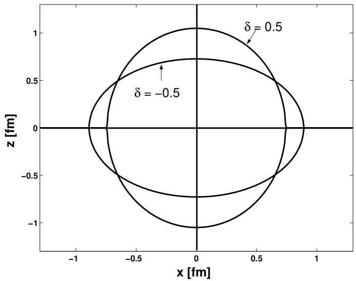
Figure 1: Plot of the ellipsoidal isocurves $V(r,\theta)=0.5$ of the deformed potential for deformation $\delta=\pm 0.5$ with potential strength $V_{0}=1$ in the $x,z$-plane. For the spherically symmetric potential a shape parameter $\alpha_{0}=1$ was chosen.

In order to assess the shape structure in more detail, it is instructive to study the multipole components of the potential. An axially symmetric potential may be expanded in terms of Legendre polynomials, i.e.

$$V(r,\theta)=\sum_{\lambda}V_{\lambda}(r)P_{\lambda}(\cos\theta).$$ (23)

Using the orthonormality properties of the Legendre polynomials, the multipole components are given by the integrals

$$V_{\lambda}(r)={(2\lambda+1)\over 2}V_{0}\exp(-\beta r^{2})\int_{-1}^{1}d\eta\>\exp(\beta\delta r^{2}\eta^{2})P_{\lambda}(\eta),$$ (24)

where $\eta=\cos(\theta)$. Here it is explicitly seen for our reflection symmetric potential, that only even multipoles give non-vanishing contributions, since the Legendre polynomials have the property

$$P_{\lambda}(-\eta)=(-1)^{\lambda}P_{\lambda}(\eta),$$

and the potential is an even function in $\eta$.

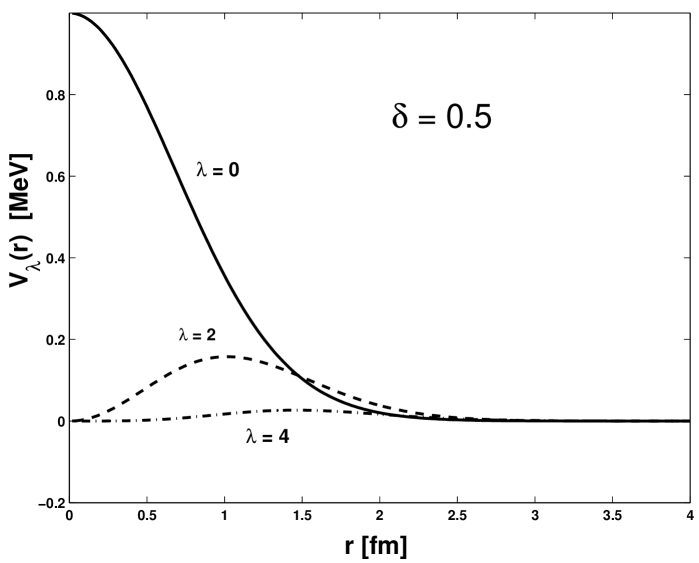
Figure 2: Plot of $\lambda=0,2,4$ multipoles of the Gaussian potential with deformation parameter $\delta=0.5$ and $\alpha_{0}=1$.

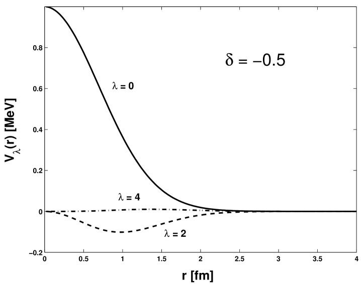
Figure 3: Plot of $\lambda=0,2,4$ multipoles of the Gaussian potential with deformation parameter $\delta=-0.5$ and $\alpha_{0}=1$.

The monopole part of the deformed Gaussian potential may be calculated analytically,

$$V_{\lambda=0}(r)={1\over 2}V_{0}\exp(-\beta r^{2})\int_{-1}^{1}d\eta\>\exp(\beta\delta r^{2}\eta^{2})={1\over 2}V_{0}\exp(-\beta r^{2})D_{0}(r),$$ (25)

where

$$D_{0}(r)={1\over 2\sqrt{\tau}}\gamma(1/2,\tau),\>\>\tau=-\beta\delta r^{2}.$$ (26)

Here $\gamma(1/2,\tau)$ is the incomplete gamma function, see e.g. Ref. Boas (1983). Figs. 2 and  3 give plots of the $\lambda=0,2,4$ multipoles of the Gaussian potential with deformation parameters $\delta=\pm 0.5$ and the potential parameters $\alpha_{0}=1$ and $V_{0}=1$. It is seen that the radial monopole distributions are more or less identical for $\delta=0.5$ and $\delta=-0.5$. Further it is seen that the deformed Gaussian potential is nearly a pure quadrupole deformation, since the $\lambda=4$ multipole is almost vanishing in both cases. This may be understood from considering the exponent of the deformed formfactor in Eq. (20), which can be rewritten in terms of the $Y_{20}(\hat{r})$ spherical harmonic.

V Multipole Components in Momentum Space.

Having discussed the shape and multipoles of the deformed Gaussian potential, we now turn to the actual solution of the Schrödinger equation for this potential. We wish to solve the partial wave decomposed momentum space Schrödinger equation given in Eq. (1), and therefore need the Gaussian deformed potential in a partial wave decomposed, momentum representation. The Fourier transformation of the deformed Gaussian potential in Eq. (18) is,

$$V(q_{x},q_{y},q_{z}) = {V_{0}\over(2\pi)^{3}}\int dx\>dy\>dz\>\exp\left(i(q_{x}x+q_{y}y+q_{z}z)\right)\exp\left(-\beta(x^{2}+y^{2})-\alpha z^{2}\right)$$ (27)

$$= {V_{0}\over 8\pi^{3/2}\beta\alpha^{1/2}}\exp\left(-{1\over 4\beta}(q_{x}^{2}+q_{y}^{2})\right)\exp\left(-{1\over 4\alpha}q_{z}^{2}\right),$$

where $q_{i}=k_{i}-k_{i}^{\prime},\>i=x,y,z$. In terms of spherical momentum space coordinates $k,\theta,\varphi$ the potential takes the form,

$$V({\bf k},{\bf k}^{\prime}) = {V_{0}\over 8\pi^{3/2}\beta\alpha^{1/2}}\exp\left(-{1\over 4\beta}(k^{2}\sin^{2}\theta+{k^{\prime}}^{2}\sin^{2}\theta^{\prime})-{1\over 4\alpha}(k\cos\theta-{k^{\prime}}\cos\theta^{\prime})^{2}\right)$$ (28)

$$\times \exp\left({1\over 2\beta}kk^{\prime}\sin\theta\sin\theta^{\prime}\cos\left(\varphi-\varphi^{\prime}\right)\right).$$

Due to axial symmetry the dependence of the potential on the azimuthal angles $\varphi,\varphi^{\prime}$ is only on the difference $\omega=\varphi-\varphi^{\prime}$. The potential may therefore be expanded in a complete set of harmonics, i.e.

$$V({\bf k},{\bf k^{\prime}})=\sum_{\mu=-\infty}^{\infty}V_{\mu}(\tilde{k},\tilde{k}^{\prime})\exp(i\mu\omega),$$ (29)

here $\tilde{k}=(k,\theta)$. The harmonics $\exp(i\mu\omega)$ obey the orthogonality relation

$$\int_{-\pi}^{\pi}d\omega\>\exp(-i\mu\omega)\exp(i\mu^{\prime}\omega)=2\pi\delta_{\mu,\mu^{\prime}},$$ (30)

the $\mu$’th harmonic of the potential is therefore given by the integral

$$V_{\mu}(\tilde{k},\tilde{k}^{\prime})={1\over 2\pi}\int_{-\pi}^{\pi}d\omega\>\exp(-i\mu\omega)V({\bf k},{\bf k}^{\prime}).$$ (31)

From Eq. (28) it is seen, that for the integral over $\omega$, we have to consider the following integral,

$$I_{\mu}(y)={1\over 2\pi}\int_{-\pi}^{\pi}d\omega\>\exp(-i\mu\omega)\exp(y\cos\omega)={1\over\pi}\int_{0}^{\pi}d\omega\>\cos(\mu\omega)\exp(y\cos\omega),$$ (32)

where we have introduced the variable

$$y={1\over 2\beta}kk^{\prime}\sin\theta\sin\theta^{\prime}.$$

The integral in Eq. (32) is just the definition of the modified Bessel function of the 1’st kind (see e.g. Abramowitz and Stegun (1972)). The $\mu$’th harmonic of the potential is thus of analytic form, and given by,

$$V_{\mu}(\tilde{k},\tilde{k}^{\prime})={V_{0}\over 8\pi^{3/2}\beta\alpha^{1/2}}\times$$

$$\exp\left(-{1\over 4\beta}(k\sin\theta-{k^{\prime}}\sin\theta^{\prime})^{2}-{1\over 4\alpha}(k\cos\theta-{k^{\prime}}\cos\theta^{\prime})^{2}\right)\exp(-y)I_{\mu}(y).$$ (33)

Inserting the expansion of the potential given in Eq. (29) into the momentum space Schrödinger Eq. (1) and projecting the equation on the harmonics $\exp(i\mu\omega)$, the three-dimensional integral equation has been reduced to an infinite set of two-dimensional integral equations. The $\mu$’th integral equation is easily solved as a matrix diagonalization problem with dimension $N_{r}\times N_{\theta}$. Here $N_{r}$ is the number of integration points for the radial integral and $N_{\theta}$ the number of integration points for the angle integral. However, the Schrödinger equation can be further reduced to a coupled set of one-dimensional integral equations by projecting on spherical harmonics (see Eq. (4)). The angular momentum projected potential in Eq. (28) then takes the form,

$$V_{lm,l^{\prime}m^{\prime}}(k,k^{\prime})=\int\mathrm{d}{\hat{k}}\int\mathrm{d}{\hat{k}^{\prime}}\>Y_{lm}^{*}(\hat{k})\left\{\sum_{\mu=-\infty}^{\infty}V_{\mu}(\tilde{k},\tilde{k}^{\prime})\exp(i\mu\omega)\right\}Y_{l^{\prime}m^{\prime}}(\hat{k}^{\prime})$$

$$=2\pi\int_{0}^{\pi}d\theta\>\sin\theta\int_{0}^{\pi}d\theta^{\prime}\>\sin\theta^{\prime}\bar{P}_{lm}(\cos\theta)V_{m}(\tilde{k},\tilde{k}^{\prime})\bar{P}_{l^{\prime}m}(\cos\theta^{\prime})\>\delta_{m,m^{\prime}},$$ (34)

where $\bar{P}_{lm}(x)$ are the normalized associated Legendre polynomial,

$$\bar{P}_{lm}(x)=\left\{{2l+1(l-m)!\over 2(l+m)!}\right\}^{1/2}P_{lm}(x).$$ (35)

In our calculations we start with the angular momentum projected potential given in Eq. (34). In numerical calculations the multipole expansion in angular momentum $l$ has to be truncated at some $l_{\mathrm{max}}$ and the Hamiltonian matrix to be diagonalized is,

$$H^{m\pi}=\left[\begin{array}[]{ccc}H^{m\pi}(l_{1},l_{1})&\ldots&H^{m\pi}(l_{1},l_{\mathrm{max}})\\ \vdots&&\vdots\\ H^{m\pi}(l_{\mathrm{max}},l_{1})&\ldots&H^{m\pi}(l_{\mathrm{max}},l_{\mathrm{max}})\end{array}\right].$$ (36)

Here $m$ and $\pi$ are the angular momentum projection and parity, respectively, which are good quantum numbers in case of axial symmetry. The allowed values of $l$ are even and odd for positive and negative parity states, respectively. Each submatrix $H^{m\pi}(l,l^{\prime})$ in Eq. (36) has matrix elements given by,

$$H^{m\pi}_{i,j}(l,l^{\prime})={\hbar^{2}\over 2\mu}k_{i}^{2}\delta_{i,j}\delta_{l,l^{\prime}}+\sqrt{w_{i}w_{j}}k_{i}k_{j}V_{lm,l^{\prime}m}(k_{i},k_{j}).$$ (37)

The rank of each submatrix $H^{m\pi}(l,l^{\prime})$ are determined by the total number of integration points used in the discretization of the integration contour $L^{+}$ in the coupled momentum space Schrödinger equation, given in Eq. (10). The results reported in this work, used the same number of integration points for each coupled equation, so the total rank of the matrix to be diagonalized is $N\times N_{l}$, where $N$ is the total number of integration points and $N_{l}$ the total number of angular momentum coupled integral equations given in Eq. (10). Diagonalizing the complex symmetric matrix (36), we obtain a complete set of states within the chosen discretization space. The basis may be utilized in different spectral represenations used in scattering theory or in Gamow-Shell-Model calculations involving deformed fields.

In all calculations reported below, we used a discretized contour $L^{+}$ defined by a rotation $\theta$ and a translation $C$ in the complex $k$-plane, see Fig. 4. In Ref. Hagen et al. (2004) it was shown that this type of contour allows for a stable numerical solutions of the scattering amplitude (or $t-$matrix), by using a spectral representation of the Green’s function. In physical scattering, the energy is given along the real axis. By defining a basis with continuum energies given along the contour depicted in Fig. 4, the problem with poles of the Green’s function are eliminated, see Ref. Hagen et al. (2004) for more details.

Figure 4: Sketch of the contour $L^{+}$ in the complex $k$-plane. The contour is specified by a rotation angle $\theta$ and a translation $C$ in the fourth quadrant of the complex $k$-plane.

The total number of integration points is given by $N=N_{R}+N_{T}$, where $N_{R}$ is the number of points along the rotated line defined by $\theta$ and $N_{T}$ is the number of points along the translated line defined by $C$. In numerical calculations $k_{\mathrm{max}}$ (see Fig. 4) should be chosen large enough, so that the calculated wave functions and energies do not change with increasing $k_{\mathrm{max}}$. In our calculations we used $k_{\mathrm{max}}=6\mathrm{fm}^{-1}$.

VI Formation of single-particle resonances in a deformed Gaussian potential.

As a model study we consider the Gaussian potential given in Eq. (17), which in the spherically symmetric case reproduces the $J^{\pi}={3/2^{-}_{1}}$ resonance in ⁵He. The $J^{\pi}={3/2^{-}_{1}}$ resonance, to be associated with the single-particle orbit $p_{3/2}$, is experimentally known to have a width of $\Gamma\approx 0.60$ MeV.

In our calculations we used the following parameters for the spherically symmetric Gaussian given in Eq. (17),

$$V_{0}=-53.5\mathrm{MeV},\>\>\alpha_{0}=0.188\mathrm{fm}^{-2}.$$ (38)

As a check of our momentum space approach, we compared our results for the spherical limit with the results obtained with the computer program GAMOW .and. K. F. Pàl .and. Z. Balogh (1982). For the spherical Gaussian potential, GAMOW gives a bound state for the $l^{\pi}=0^{+}$ channel with energy $E=-14.9044$MeV, and a resonance for the $l^{\pi}=1^{-}$ channel with energy $E=0.7268-0.3096i$MeV. Here the nucleon spin $s=1/2$ is neglected since the energy levels are degenerate for $j=l\pm 1/2$, which follows from the spin independence of the Gaussian potential. Our momentum space calculations were able to exactly reproduce these results with a total number of discretization points $N=25$. This comparison of two different methods, provided us with a check of our codes and our derivation of the momentum space equations.

In order to obtain converged results for the deformed case, we investigate the convergence with respect to total number angular momentum coupled equations, see Eq. (36), and with respect to the total number of integration points used in discretization of each coupled integral equation given in Eq.(10). First, convergence with respect to total number angular momentum coupled equations in Eq. (36) is considered. We fixed the number of integration points to $N=N_{R}+N_{T}=20+30=50$, this is large enough to ensure convergence with respect to number of discretization points. For bound states we used a real contour $L^{+}$, i.e. $\theta=0$ and the real $k-$axis was discretized with 50 points. In the case of resonant states we used a complex contour $L^{+}$ defined by a rotation $\theta=\pi/4$ and a translation $C=\sin(\pi/4)\times 0.4\mathrm{fm}^{-1}\sim-0.29\mathrm{fm}^{-1}$ in the complex $k$-plane (see Fig. 4).

Table 1 gives the convergence of the $m^{\pi}=0^{+}$ ground state energy, for deformation parameters $\delta=\pm 0.9$. For $\delta=-0.9$, convergence is quickly reached, with $l_{\mathrm{max}}=4$. For $\delta=0.9$, convergence is considerably slower. It is seen that the deformation $\delta=0.9$ affects the bound state most, and the ground state becomes less bound $E=-12.1$MeV, for the prolate deformation. On the other hand, the oblate deformation $\delta=-0.9$ has little effect on the ground state energy $E=-14.7$MeV.

	$\delta=0.9$		$\delta=-0.9$
$l_{\mathrm{max}}$	Re[E]	Im[E]	Re[E]	Im[E]
0	-10.5843	0.	-14.4816	0.
2	-11.9041	0.	-14.6533	0.
4	-12.0741	0.	-14.6551	0.
6	-12.0953	0.	-14.6551	0.
8	-12.0979	0.	-14.6551	0.
10	-12.0983	0.	-14.6551	0.

Table 1: Convergence of groundstate, $m^{\pi}=0^{+}$, for deformation parameters $\delta=\pm 0.9$ as the number of partial waves increases. In the spherically symmetric case $\delta=0$ the $l^{\pi}=0^{+}$ Gaussian potential supports a bound state at energy $E=-14.9044$MeV.

This may be understood by considering the monopole term of the potential, which is the main component in the multipole expansion in Eq. (23). In Fig. 5 a plot of the monopole part of the Gaussian potential with deformation parameters $\delta=\pm 0.9$ is given, together with a plot of the spherically symmetric potential. It is seen that the monopole term for the $\delta=-0.9$ potential is more or less identical to the spherically symmetric potential (slightly less attractive), on the other hand the monopole term for the $\delta=0.9$ potential is less attractive for $r<4$fm, but more attractive at large distances $r>4$fm. From this one may conclude that the ground state of the $\delta=-0.9$ potential will be more bound than for the $\delta=0.9$ potential, since the ground state is deeply bound and the wave function will be mainly located in the interior part of the potential.

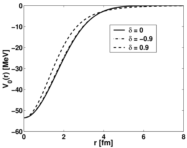
Figure 5: Plot of the monopole part of the Gaussian potential with deformation parameters $\delta=0$ and $\delta=\pm 0.9$.

The resonant orbit $l^{\pi}=1^{-}$ in the spherically symmetric potential is split into two non-degenerate orbits ( $m^{\pi}=0^{-}$ and $m^{\pi}=1^{-}$) in the case of an axially symmetric deformation. This is a characteristic of axially deformed potentials. Table 2 gives the convergence of the $m^{\pi}=0^{-}$ and $m^{\pi}=1^{-}$ excited negative parity states in the Gaussian potential, for deformation parameters $\delta=\pm 0.5$. In all cases a satisfactory convergence is obtained with $l_{\mathrm{max}}=5$. For the states with vanishing angular momentum projection along the $z$-axis ( $m=0$ ), it is seen that for $\delta=0.5$ ( prolate deformation ) the $l^{\pi}=1^{-}$ state has become a bound state with energy $E=-0.680$MeV. For zero angular momentum projection, the particle moves in an orbit along the $z$-axis. So in the case of a prolate deformation, where the field is stretched out along the $z$-axis, a particle moving in this orbit will “feel” the field more strongly than compared with the spherically symmetric field, and it will become more bound. This explains also why the particle with $m=0$ becomes more unbound in the case of the oblate deformation $\delta=-0.5$, see Columns 6 and 7 of Table 2.

	$\delta=0.5$				$\delta=-0.5$
	$m^{\pi}=0^{-}$		$m^{\pi}=1^{-}$		$m^{\pi}=0^{-}$		$m^{\pi}=1^{-}$
$l_{\mathrm{max}}$	Re[E]	Im[E]	Re[E]	Im[E]	Re[E]	Im[E]	Re[E]	Im[E]
1	-0.5282	0.	1.4865	-1.0177	1.5402	-1.0701	0.3815	-0.1139
3	-0.6772	0.	1.4419	-0.9631	1.5170	-1.0404	0.3602	-0.1042
5	-0.6802	0.	1.4410	-0.9621	1.5168	-1.0402	0.3601	-0.1041
7	-0.6803	0.	1.4410	-0.9620	1.5168	-1.0402	0.3601	-0.1041
9	-0.6803	0.	1.4410	-0.9620	1.5168	-1.0402	0.3601	-0.1041

Table 2: Convergence of the $m^{\pi}=0^{-}$ and $m^{\pi}=1^{-}$ energies, for deformation parameters $\delta=\pm 0.5$ with increasing number of partial waves. In the spherically symmetric case ($\delta=0$) the $l^{\pi}=1^{-}$ Gaussian potential supports a resonance state at energy $E=0.7268-0.3096i$MeV.

	$\delta=0.5$				$\delta=-0.5$
	$m^{\pi}=0^{-}$		$m^{\pi}=1^{-}$		$m^{\pi}=0^{-}$		$m^{\pi}=1^{-}$
$l_{\mathrm{max}}$	Re[$\psi_{l}^{2}$ ]	Im[$\psi_{l}^{2}$]	Re[$\psi_{l}^{2}$ ]	Im[$\psi_{l}^{2}$]	Re[$\psi_{l}^{2}$ ]	Im[$\psi_{l}^{2}$]	Re[$\psi_{l}^{2}$ ]	Im[$\psi_{l}^{2}$]
1	0.9947	0.	0.9982	2.31E-03	0.9992	1.1E-03	0.9993	3.E-04
3	5.7E-03	0.	1.8E-03	-2.3E-03	8.E-04	-1.1E-03	7.E-04	-3.E-04
5	5.E-05	0.	2.E-05	-2.E-05	3.E-06	-3.E-06	2.E-06	-9.E-07
7	6.E-07	0.	3.E-07	-2.E-07	2.E-08	-1.E-08	9.E-09	-4.E-09
9	8.E-09	0.	4.E-09	-3.E-09	9.E-11	-7.E-11	4.E-11	-2.E-11

Table 3: Convergence of the $m^{\pi}=0^{-}$ and $m^{\pi}=1^{-}$ squared amplitudes of the wave functions for each partial wave $l$, for deformation parameters $\delta=\pm 0.5$.

For the $m=1$ case the opposite takes place. In the case of $\delta=0.5$ the particle becomes more unbound, while for $\delta=-0.5$ the particle becomes more bound. By considering the dipole ($l=1$) term of the wave function, the particle moves in an orbit making $\pi/4$ degrees with the $z$-axis. From this it may be understood that the particle gains more binding in the case of an oblate deformation $\delta=-0.5$ and becomes more un-physical in the opposite case $\delta=0.5$ ( see columns 4,5,8 and 9 of table 2).

In table 3 the squared amplitudes of the wave functions are given for each partial wave $l$. It is seen that in all cases that the squared amplitudes for the $l=1$ component of the total wave function, is nearly equal to the norm of the total wave function, while all other partial wave amplitudes are vanishing small. In this sense one may say that the orbital angular momentum is approximately a “good” quantum number.

Having investigated the convergence with respect to number of angular momentum coupled equations, we now consider convergence with respect to number of discretization points along the contour $L^{+}$, for the negative parity states. For the energies in Tables 2 and 3, we reached satisfactory convergence with $l_{\mathrm{max}}=7$. In considering convergence with respect to integration points, we then fix the maximum number of coupled equation to $l_{\mathrm{max}}=7$. Table 4 reports the convergence of the odd parity energies in the deformed Gaussian potential given in Eq. (28), with deformation parameters $\delta=\pm 0.5$.

		$\delta=0.5$				$\delta=-0.5$
		$m^{\pi}=0^{-}$		$m^{\pi}=1^{-}$		$m^{\pi}=0^{-}$		$m^{\pi}=1^{-}$
$N_{R}$	$N_{T}$	Re[E]	Im[E]	Re[E]	Im[E]	Re[E]	Im[E]	Re[E]	Im[E]
5	10	-0.6777	0.0000	1.4392	-0.9680	1.5150	-1.0472	0.3576	-0.1091
10	10	-0.6777	0.0000	1.4401	-0.9656	1.5150	-1.0448	0.3577	-0.1091
10	15	-0.6803	0.0000	1.4411	-0.9621	1.5170	-1.0403	0.3601	-0.1043
10	20	-0.6803	0.0000	1.4410	-0.9620	1.5168	-1.0402	0.3601	-0.1041
10	25	-0.6803	0.0000	1.4410	-0.9620	1.5168	-1.0402	0.3601	-0.1041
15	25	-0.6803	0.0000	1.4410	-0.9620	1.5168	-1.0402	0.3601	-0.1041
15	30	-0.6803	0.0000	1.4410	-0.9620	1.5168	-1.0402	0.3601	-0.1041
20	30	-0.6803	0.0000	1.4410	-0.9620	1.5168	-1.0402	0.3601	-0.1041

Table 4: Convergence of the $m^{\pi}=0^{-}$ and $m^{\pi}=1^{-}$ energies with increasing number of discretization points along the contour $L^{+}$. Here deformation parameters $\delta=\pm 0.5$ were used, and $l_{\mathrm{max}}=7$.

It is seen that one obtains convergence with a total number of integration points given by $N=N_{R}+N_{T}=10+20=30$. Note also that with $N=15$ points, we have satisfactory results. For $N=30$ and $N_{l}=4$ (only four coupled equations for $l_{\mathrm{max}}=7$ due to conservation of parity) the total dimension of the matrix in Eq. (36) is $dim=120$, which is diagonalized extremely fast with any diagonalization routine suitable for complex symmetric matrices.

Having determined convergence properties of the odd and even parity states in the deformed Gaussian potential, we now study how the different states behave over a large range of deformations. In figure (6) a plot of the bound state energy of the $m^{\pi}=0^{+}$ state is given for the deformation parameter $\delta$ taking values between $-0.9$ and $0.9$. It is seen that the position of the bound state varies much more strongly for a prolate deformation ($\delta>0$), than for an oblate deformation.

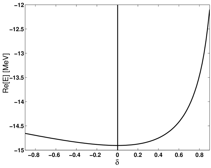
Figure 6: Bound state trajectory for the $m^{\pi}=0^{+}$ state in the deformed Gaussian potential. Energy is plotted as function of deformation parameter $\delta$.

Fig. 7 shows a plot of the real (solid lines) and imaginary part (dashed lines) of the $m^{\pi}=0^{-}$ and $m^{\pi}=1^{-}$ states for the deformation parameter $\delta$ taking values between $-0.9$ and $0.9$.

The value for $\delta$ in which the $m^{\pi}=0^{-}$ resonant state becomes a bound state is given when the real energy trajectory meets the imaginary energy trajectory for $\mathrm{Re}[E]<0$, i.e. $\mathrm{Im}[E]=\mathrm{Re}[E]$. Here the splitting of the $l^{\pi}=1^{-}$ resonant level with respect to the angular momentum projection $m$ is clearly seen. It is also seen that the energy of the $m^{\pi}=0^{-}$ and the $m^{\pi}=1^{-}$ state behave in opposite manner for $\delta>0$ and for $\delta<0$. The $m^{\pi}=0^{-}$ resonance for $\delta=0$ becomes a bound state for $\delta>0.3$. For $\delta<0$ the $m^{\pi}=0^{-}$ resonance moves further down in the lower half complex $k$-plane. On the other hand, it is seen that the $m^{\pi}=1^{-}$ resonance state does not become a bound state for the values of $\delta$ considered, $\delta\in(-0.9,0.9)$. For $\delta\in(-0.9,0.2)$ the $m^{\pi}=1^{-}$ resonance energy displays a weak variation from the $\delta=0$ energy, and slowly moves towards the scattering threshold $E=0$, for $\delta\rightarrow-0.9$. On the other hand, as $\delta\rightarrow 0.9$ the imaginary part of the energy dives into the lower half complex energy plane, and the resonance state becomes strongly unphysical.

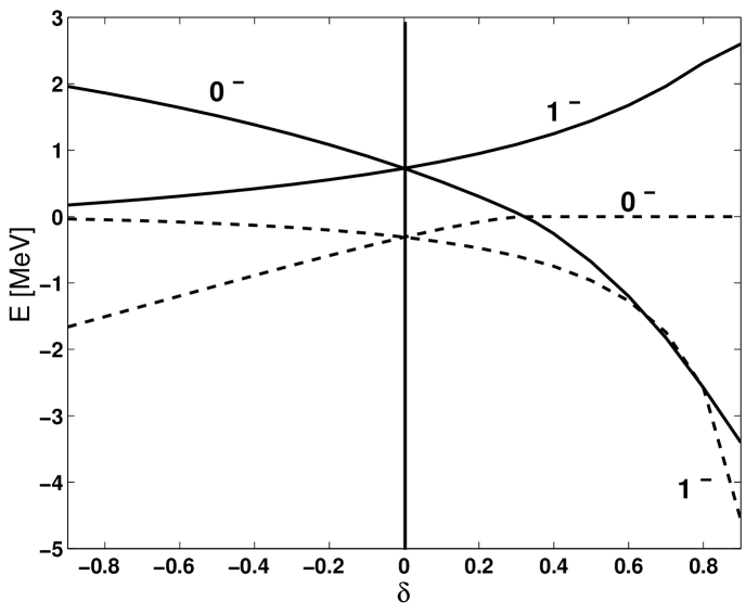
Figure 7: Real (solid lines) and imaginary parts (dashed lines) of the $m^{\pi}=0^{-}$ and the $m^{\pi}=1^{-}$ state energies in the deformed Gaussian potential as the deformation parameter $\delta$ is varied between $-0.9$ and $0.9$.

VII Conclusion.

In this work, we have demonstrated that the Contour Deformation Method may be generalized to the case of deformed potentials. CDM is applied to the momentum space Schrödinger equation, allowing for stable and converged solutions of physical resonances. In addition a complete set of Berggren states is obtained, which may be used in the construction of a many-body Berggren basis. The most obvious advantage of this momentum space approach, as compared to its position space analog, is that the boundary conditions of all kinds of states, i.e. bound, resonant and continuum, are automatically taken care of since we are dealing with integral equations instead of integro-differential equations. The method is demonstrated for axial symmetry and a fictitious ”deformed ⁵He”, but may be extended to more general deformation and applied to truly deformed halo nuclei. Such applications as to ⁸Li, ⁹Be and ¹¹Be will be discussed elsewhere.

References

- Michel et al. (2004a) N. Michel, W. Nazarewicz, and M. Płoszajczak, Phys. Rev. C 70, 064313 (2004a).
- Michel et al. (2004b) N. Michel, W. Nazarewicz, M. Płoszajczak, and J. Rotureau, nucl-th/0401036 (2004b).
- Dobaczewski et al. (2004) J. Dobaczewski, N. Michel, W. Nazarewicz, M. Płoszajczak, and M. V. Stoitsov, nucl-th/0401034 (2004).
- Michel et al. (2002) N. Michel, W. Nazarewicz, M. Ploszajczak, and K. Bennaceur, Phys. Rev. Lett. 89, 042502 (2002).
- Michel et al. (2003) N. Michel, W. Nazarewicz, M. Ploszajczak, and J. Okołowicz, Phys. Rev. C 67, 054311 (2003).
- IdBetan et al. (2002) R. IdBetan, R. J. Liotta, N. Sandulescu, and T. Vertse, Phys. Rev. Lett. 89, 042501 (2002).
- IdBetan et al. (2003) R. IdBetan, R. J. Liotta, N. Sandulescu, and T. Vertse, Phys. Rev. C 67, 014322 (2003).
- IdBetan et al. (2004) R. IdBetan, R. J. Liotta, N. Sandulescu, and T. Vertse, Phys. Lett. B 584, 48 (2004).
- Hagen et al. (2004) G. Hagen, J. S. Vaagen, and M. Hjorth-Jensen, J. Phys. A: Math. Gen. 37, 8991 (2004).
- Hagen et al. (2005) G. Hagen, M. Hjorth-Jensen, and J. S. Vaagen, Phys. Rev. C 71, 044314 (2005).
- Berggren (1968) T. Berggren, Nucl. Phys. A 109, 265 (1968).
- Berggren (1971) T. Berggren, Nucl. Phys. A 169, 353 (1971).
- Berggren (1978) T. Berggren, Phys. Lett. B 73, 389 (1978).
- Berggren (1996) T. Berggren, Phys. Lett. B 373, 1 (1996).
- Lind (1993) P. Lind, Phys. Rev. C 47, 1903 (1993).
- Kruppa et al. (2004) A. T. Kruppa, N. Michel, and W. Nazarewicz, CP726, Nuclear Physics, Large and Small: International Conference on Microscopic Studies of Collective Phenomena p. 7 (2004).
- Ferreira et al. (1997) L. Ferreira, E. Maglione, and R. J. Liotta, Phys. Rev. Lett. 78, 1640 (1997).
- Hagino and Giai (2004) K. Hagino and N. V. Giai, Nucl. Phys. A 735, 55 (2004).
- Biedenharn and Dam (1965) L. C. Biedenharn and H. V. Dam, Quantum Theory of Angular Momentum : A Collection of Reprints and Original Papers (New York : Academic Press, 1965).
- Gradshteyn and Ryzhik (1963) I. S. Gradshteyn and I. M. Ryzhik, Table of Integrals Series and Products (Academic Press Inc., 1963), 4th ed.
- Abramowitz and Stegun (1972) M. Abramowitz and I. A. Stegun, Handbook of Mathematical Functions (Dover Publications, Inc., New York, 1972).
- Boas (1983) M. L. Boas, Mathematical Methods in the Physical Sciences (John Wiley and Sons, Inc, 1983), 2nd ed.
- .and. K. F. Pàl .and. Z. Balogh (1982) T. V. .and. K. F. Pàl .and. Z. Balogh, Comput. Phys. Commun. 27, 309 (1982).