Relativistic eikonal description of $A(p,pN)$ reactions

Abstract

The authors present a relativistic and cross-section factorized framework for computing quasielastic $A(p,pN)$ observables at intermediate and high energies. The model is based on the eikonal approximation and can accomodate both optical potentials and the Glauber method for dealing with the initial- and final-state interactions (IFSI). At lower nucleon energies, the optical-potential philosophy is preferred, whereas at higher energies the Glauber method is more natural. This versatility in dealing with the IFSI allows one to describe $A(p,pN)$ reactions in a wide energy range. Most results presented here use optical potentials as this approach is argued to be the optimum choice for the kinematics of the experiments considered in the present paper. The properties of the IFSI factor, a function wherein the entire effect of the IFSI is contained, are studied in detail. The predictions of the presented framework are compared with two kinematically different experiments. First, differential cross sections for quasielastic proton scattering at $1$ GeV off ¹²C, ¹⁶O, and ⁴⁰Ca target nuclei are computed and compared to data from PNPI. Second, the formalism is applied to the analysis of a ⁴He$(p,2p)$ experiment at $250$ MeV. The optical-potential calculations are found to be in good agreement with the data from both experiments, showing the reliability of the adopted model in a wide energy range.

I Introduction

Quasielastic nucleon knockout reactions have been extensively investigated with the aim of obtaining precise information on nuclear structure. The present work focuses on exclusive proton-induced $A(p,2p)$ and $A(p,pn)$ processes, whereby the residual A-1 nucleus is left in the discrete part of its energy spectrum. A sketch of the $A(p,2p)$ reaction is given in Fig. 1. For a historical overview of the research into proton-induced nucleon emission off nuclear targets the reader is referred to Refs. jacob66 ; jacob73 ; kitching85 .

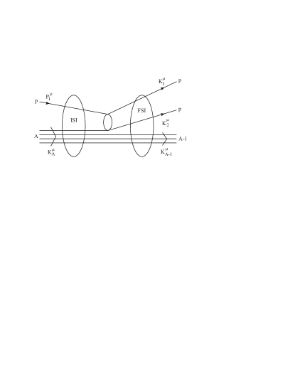
Figure 1: Schematic representation of the $A(p,2p)$ reaction. The incoming proton undergoes “soft” initial-state interactions with the target before knocking out a bound proton through the primary high-momentum-transfer $pp$ scattering. Both the scattered and the ejected proton suffer final-state interactions while leaving the nucleus. The scattered and the ejected proton are detected in coincidence, while the residual nucleus remains unobserved.

In quasielastic $A(p,pN)$ scattering the projectile is elastically scattered from a single bound nucleon in the target nucleus, resulting in the struck nucleon being knocked out of the target nucleus. This relatively simple reaction mechanism of one “hard” nucleon-nucleon collision is obscured by the “soft” initial- and final-state interactions (IFSI) of the incident and two outgoing nucleons with the nuclear medium. Consequently, every model for $A(p,2p)$ and $A(p,pn)$ reactions has two issues to address : first, the description of the “hard” wide-angle scattering that leads to the ejection of the struck nucleon and second, the distorting mechanisms of the “soft” small-angle IFSI.

Concerning the treatment of the “hard” $NN$ scattering part, essentially two methods exist. A so-called “cross-section factorized” approximation jacob66 ; chant77 can be adopted so that the nucleon-nucleon scattering cross section enters as a multiplicative factor in the differential $A(p,pN)$ cross section. Some results of exclusive $A(p,2p)$ measurements interpreted with this cross-section factorized form can be found in Refs. kullander71 ; bhowmik74 ; bengtsson78 ; kitching80 ; oers82 ; carman99 . The inclusion of spin-dependence in the description of the IFSI, however, breaks this factorization scheme. In that situation an alternative technique can be used : the amplitude factorized form of the cross section chant83 . In this approach, the two-body $NN$ interaction can be approximated by the interpolation of phase shifts SAID from free elastic $NN$ scattering. Various phenomenological forms to fit the amplitudes have also been used in the past. Traditionally, the nucleon-nucleon scattering matrix has been parametrized in terms of five Lorentz invariants mcneil ; horowitz ; maxwell , a method usually dubbed as the IA1 model or the SPVAT (scalar, pseudoscalar, vector, axial vector, tensor) form of the $NN$ scattering matrix. Differential cross section calculations adopting these five-term representations have been reported in Refs maxwellcooper ; ikebata95 ; mano98 ; miller98 ; neveling02 . It should be noted, however, that although the SPVAT form gives reasonable predictions of $A(p,pN)$ observables, it is, in principle, not correct, as a five-term parametrization of the relativistic $NN$ scattering matrix is inherently ambiguous adams84 . Tjon and Wallace tjon85 have shown that a complete expansion of the $NN$ scattering matrix (commonly called the IA2 model) contains $44$ independent invariant amplitudes. To date, the only calculations employing this general Lorentz invariant representation have been performed in the context of the relativistic plane wave impulse approximation (RPWIA), i.e., a model which ignores all IFSI mechanisms vanderventel04 .

The IFSI effects are typically computed by means of the distorted wave impulse approximation (DWIA) theoretical framework jackson65 ; chant77 ; chant83 ; kitching85 . Generally, in a DWIA approach the scattering wave functions of the incoming and two outgoing nucleons are generated by solving the Schrödinger or Dirac equation with complex optical potentials. Parametrizations for these optical potentials are usually not gained from basic grounds, but are obtained by fitting elastic nucleon-nucleus scattering data. Several optical-potential parameter sets nadasen81 ; oers82 ; schwandt82 ; madland87 ; cooper87 ; cooper88 ; hama90 ; cooper93 have been used in the description of quasifree proton scattering off nuclei. In the past, both nonrelativistic and relativistic DWIA versions kullander71 ; bhowmik74 ; kitching80 ; antonuk81 ; oers82 ; samanta86 ; cowley91 ; cowley95 ; ikebata95 ; miller98 ; cowley98 ; mano98 ; carman99 ; neveling02 ; maxwellcooper have proven successful in predicting $A(p,pN)$ cross sections over a wide energy range ($76$–$600$ MeV) and for a whole scope of target nuclei.

Most of the available calculations for the exclusive $A(p,pN)$ process addressed incident proton kinetic energies of a few hundred MeV. In this work we aim at extending the formalism to scattering in the GeV energy regime. As a matter of fact, the majority of DWIA frameworks rely on partial-wave expansions of the exact solution to the scattering problem, an approach which becomes increasingly cumbersome at higher energies. In this energy range the eikonal approximation mccauley58 ; joachain75 , which belongs to the class of high-energy semiclassical methods, offers a valid alternative for describing the IFSI. Nonrelativistic eikonal studies of the $A(p,2p)$ reaction used in combination with optical potentials can be found in Refs. jacob66 ; kullander71 ; bengtsson78 .

In this paper we propose a relativistic and cross-section factorized formalism based on the eikonal approximation for computing exclusive $A(p,pN)$ cross sections at incident proton energies in the few hundred MeV to GeV range. The eikonal formalism is implemented relativistically in combination with optical potentials cooper93 , as well as with Glauber theory glauber70 ; wallace75 ; yennie71 , which is a multiple-scattering extension of the eikonal approximation. The two frameworks only differ in the way they treat the IFSI. The main focus will be on the optical-potential approach, as this method turns out to be the most suitable for the description of the IFSI for the kinematical settings discussed in this work.

The paper is organized as follows. In Secs. II.1 and II.2 the factorized cross section is derived in the RPWIA formalism. Thereafter, the different methods to deal with the IFSI are developed in Sec. II.3. Sec. III is devoted to a presentation of optical-potential and Glauber results for the IFSI factor. This is a function which accounts for all IFSI effects when computing the $A(p,pN)$ observables. The optical-potential predictions of our model are compared with cross section data that have been collected at PNPI and TRIUMF in Sec. IV. First, we present our calculations for the ¹²C, ¹⁶O, and ⁴⁰Ca$(p,2p)$ and $(p,pn)$ PNPI data for $1$ GeV incoming proton energies belostotsky87 . Second, the cross sections for ⁴He$(p,2p)$ scattering at $250$ MeV are compared to the TRIUMF data by van Oers et al. oers82 . Finally, Sec. V states our conclusions.

II $A(p,2p)$ formalism

In this section the formalism for the description of $A(p,2p)$ reactions is outlined. The generalization to $A(p,pn)$ reactions is straightforward. We conform to the conventions of Bjorken and Drell bjorken64 for the $\gamma$ matrices and the Dirac spinors, and take $\hbar=c=1$.

II.1 $A(p,2p)$ differential cross section and matrix element

The four-momenta of the incident and scattered proton are denoted as $P^{\mu}_{1}(E_{p1},\vec{p}_{1})$ and $K^{\mu}_{1}(E_{k1},\vec{k}_{1})$. The proton momenta $\vec{p}_{1}$ and $\vec{k}_{1}$ define the scattering plane. The four-momentum transfer is given by $(\omega,\vec{q})\equiv q^{\mu}=P^{\mu}_{1}-K^{\mu}_{1}=K_{A-1}^{\mu}+K_{2}^{\mu}-K_{A}^{\mu}$, where $K_{A}^{\mu}(E_{A},\vec{k}_{A})$, $K_{A-1}^{\mu}(E_{A-1},\vec{k}_{A-1})$, and $K_{2}^{\mu}(E_{k2},\vec{k}_{2})$ are the four-momenta of the target nucleus, residual nucleus, and the ejected proton. The standard convention $Q^{2}\equiv-q_{\mu}q^{\mu}=\left|\vec{q}\right|^{2}-\omega^{2}\geq 0$ is followed for the four-momentum transfer.

In the laboratory frame, the fivefold differential cross section can be written as

$$\left(\frac{d^{5}\sigma}{dE_{k1}d\Omega_{1}d\Omega_{2}}\right)=\frac{M_{p}^{3}M_{A-1}}{(2\pi)^{5}M_{A}}\frac{k_{1}k_{2}}{p_{1}}f_{rec}^{-1}\>\overline{\sum_{if}}\left|{\cal M}_{fi}^{(p,2p)}\right|^{2}\;.$$ (1)

Here, ${\cal M}_{fi}^{(p,2p)}$ is the invariant matrix element which reflects the transition between the initial and final states. The hadronic recoil factor is given by

$$f_{rec}=\frac{E_{A-1}}{E_{A}}\left|1+\frac{E_{k2}}{E_{A-1}}\left(1-\frac{\vec{q}\cdot\vec{k}_{2}}{k_{2}^{2}}\right)\right|=\left|1+\frac{\omega k_{2}-qE_{k2}\cos\theta_{k_{2}q}}{M_{A}k_{2}}\right|\;,$$ (2)

with the energy transfer $\omega=E_{p1}-E_{k1}=E_{A-1}+E_{k2}-E_{A}$, the three-momentum transfer $\vec{q}=\vec{p}_{1}-\vec{k}_{1}=\vec{k}_{A-1}+\vec{k}_{2}-\vec{k}_{A}$, and $\theta_{k_{2}q}$ the angle between $\vec{k}_{2}$ and $\vec{q}$.

The $A(p,2p)$ matrix element is given by

$${\cal M}_{fi}^{(p,2p)}=\left<K^{\mu}_{1}\>m_{s1f},\;K^{\mu}_{2}\>m_{s2f},\;\mbox{A-1}\>(K_{A-1}^{\mu},\>J_{R}\>M_{R})\right|\widehat{\mathcal{O}}^{(2)}\left|P^{\mu}_{1}\>m_{s1i},\;A\>(K_{A}^{\mu},\;0^{+},\;g.s.)\right>\;,$$ (3)

where

$$\widehat{\mathcal{O}}^{(2)}=\sum_{i<j=0}^{A}O\left(\vec{r}_{i},\vec{r}_{j}\right)$$ (4)

is the unknown two-body operator describing the high-momentum transfer “hard” $pp$ scattering, $\left|A\>(K_{A}^{\mu},\;0^{+},\;g.s.)\right>$ the ground state of the even-even target nucleus and $\left|\mbox{A-1}\>(K_{A-1}^{\mu},\>J_{R}\>M_{R})\right>$ the discrete state in which the residual nucleus is left. In coordinate space the matrix element takes on the form

$${\cal M}_{fi}^{(p,2p)} = \int d\vec{r}_{0}\int d\vec{r}_{1}\int d\vec{r}_{2}\ldots\int d\vec{r}_{A}\left(\Psi^{\vec{k}_{1},m_{s1f},\vec{k}_{2},m_{s2f}}_{A+1}\left(\vec{r}_{0},\vec{r}_{1},\vec{r}_{2},\ldots,\vec{r}_{A}\right)\right)^{\dagger}\widehat{\mathcal{O}}^{(2)}$$ (5)

$$\times\>\Psi^{\vec{p}_{1},m_{s1i},gs}_{A+1}\left(\vec{r}_{0},\vec{r}_{1},\vec{r}_{2},\ldots,\vec{r}_{A}\right)\;.$$

For the sake of brevity of the notations, only the spatial coordinates are explicitly written.

II.2 Relativistic plane wave impulse approximation

In this section, the $A(p,2p)$ matrix element of Eq. (5) will be analyzed in the RPWIA. In this approach, only one hard collision between the projectile and a bound nucleon is assumed to occur, knocking the bound nucleon out of the target nucleus. The modelling of the “soft” IFSI processes, which affect both the incoming and outgoing protons, will be considered in Sec. II.3.

In evaluating the $A(p,2p)$ matrix element of Eq. (5), a mean-field approximation for the nuclear wave functions is adopted. We also assume factorization between the “hard” $NN$ coupling and the nuclear dynamics. For reasons of conciseness, the forthcoming derivations are explained for the $A=3$ case. The generalization to arbitrary mass number $A$ is rather straightforward.

The antisymmetrized (A+1)-body wave function in the initial state is of the Slater determinant form

$$\Psi^{\vec{p}_{1},m_{s1i},gs}_{A+1}\left(\vec{r}_{0},\vec{r}_{1},\vec{r}_{2},\vec{r}_{3}\right)=\frac{1}{\sqrt{(A+1)!}}\left|\begin{array}[]{cccc}\phi_{\vec{p}_{1}m_{s1i}}\left(\vec{r}_{0}\right)&\phi_{\alpha_{1}}\left(\vec{r}_{0}\right)&\phi_{\alpha_{2}}\left(\vec{r}_{0}\right)&\phi_{\alpha_{3}}\left(\vec{r}_{0}\right)\\ \phi_{\vec{p}_{1}m_{s1i}}\left(\vec{r}_{1}\right)&\phi_{\alpha_{1}}\left(\vec{r}_{1}\right)&\phi_{\alpha_{2}}\left(\vec{r}_{1}\right)&\phi_{\alpha_{3}}\left(\vec{r}_{1}\right)\\ \phi_{\vec{p}_{1}m_{s1i}}\left(\vec{r}_{2}\right)&\phi_{\alpha_{1}}\left(\vec{r}_{2}\right)&\phi_{\alpha_{2}}\left(\vec{r}_{2}\right)&\phi_{\alpha_{3}}\left(\vec{r}_{2}\right)\\ \phi_{\vec{p}_{1}m_{s1i}}\left(\vec{r}_{3}\right)&\phi_{\alpha_{1}}\left(\vec{r}_{3}\right)&\phi_{\alpha_{2}}\left(\vec{r}_{3}\right)&\phi_{\alpha_{3}}\left(\vec{r}_{3}\right)\end{array}\right|\;.$$ (6)

Details on the bound-state single-particle wave functions $\phi_{\alpha_{i}}\left(\vec{r},\vec{\sigma}\right)$ entering this mean-field (A+1)-body wave function can be found in Appendix A. The wave function of the incoming proton is given by a relativistic plane wave

$$\phi_{\vec{k}m_{s}}\left(\vec{r}\right)\equiv\sqrt{\frac{E+M}{2M}}\left[\begin{array}[]{c}1\\ \frac{1}{E+M}\vec{\sigma}\cdot\hat{\vec{p}}\end{array}\right]e^{i\vec{k}\cdot\vec{r}}\chi_{\frac{1}{2}m_{s}}=e^{i\vec{k}\cdot\vec{r}}\>u(\vec{k},m_{s})\;.$$ (9)

The (A+1)-body wave function in the final state reads

$$\Psi^{\vec{k}_{1},m_{s1f},\vec{k}_{2},m_{s2f}}_{A+1}\left(\vec{r}_{0},\vec{r}_{1},\vec{r}_{2},\vec{r}_{3}\right)=\frac{1}{\sqrt{(A+1)!}}\left|\begin{array}[]{cccc}\phi_{\vec{k}_{1}m_{s1f}}\left(\vec{r}_{0}\right)&\phi_{\vec{k}_{2}m_{s2f}}\left(\vec{r}_{0}\right)&\phi_{\alpha_{2}}\left(\vec{r}_{0}\right)&\phi_{\alpha_{3}}\left(\vec{r}_{0}\right)\\ \phi_{\vec{k}_{1}m_{s1f}}\left(\vec{r}_{1}\right)&\phi_{\vec{k}_{2}m_{s2f}}\left(\vec{r}_{1}\right)&\phi_{\alpha_{2}}\left(\vec{r}_{1}\right)&\phi_{\alpha_{3}}\left(\vec{r}_{1}\right)\\ \phi_{\vec{k}_{1}m_{s1f}}\left(\vec{r}_{2}\right)&\phi_{\vec{k}_{2}m_{s2f}}\left(\vec{r}_{2}\right)&\phi_{\alpha_{2}}\left(\vec{r}_{2}\right)&\phi_{\alpha_{3}}\left(\vec{r}_{2}\right)\\ \phi_{\vec{k}_{1}m_{s1f}}\left(\vec{r}_{3}\right)&\phi_{\vec{k}_{2}m_{s2f}}\left(\vec{r}_{3}\right)&\phi_{\alpha_{2}}\left(\vec{r}_{3}\right)&\phi_{\alpha_{3}}\left(\vec{r}_{3}\right)\end{array}\right|\;.$$ (10)

Relative to the target nucleus ground state written in Eq. (6), the wave function of Eq. (10) refers to the situation whereby the struck proton resides in a state “$\alpha_{1}$”, leaving the residual A-1 nucleus as a hole state in that particular single-particle level. The outgoing protons are represented by relativistic plane waves.

Since both the initial and the final wave functions are fully antisymmetrized, one can choose the operator $\widehat{\mathcal{O}}^{(2)}$ to act on two particular coordinates ($\vec{r}_{0}$ and $\vec{r}_{1}$). Without any loss of generality, the $A(p,2p)$ matrix element of Eq. (5) can be written as

$${\cal M}_{fi}^{(p,2p)} = \frac{A(A+1)}{2}\frac{1}{(A+1)!}\int d\vec{r}_{0}\int d\vec{r}_{1}\int d\vec{r}_{2}\int d\vec{r}_{3}$$ (11)

$$\times\>\sum_{k,l\in\left\{\vec{k}_{1}m_{s1f},\vec{k}_{2}m_{s2f}\right\}}\;\;\sum_{m,n\in\left\{\alpha_{2},\alpha_{3}\right\}}\;\;\sum_{o,p\in\left\{\vec{p}_{1}m_{s1i},\alpha_{1}\right\}}\;\;\sum_{q,r\in\left\{\alpha_{2},\alpha_{3}\right\}}$$

$$\times\>\epsilon_{klmn}\epsilon_{opqr}\phi_{k}^{\dagger}\left(\vec{r}_{0}\right)\phi_{l}^{\dagger}\left(\vec{r}_{1}\right)\phi_{m}^{\dagger}\left(\vec{r}_{2}\right)\phi_{n}^{\dagger}\left(\vec{r}_{3}\right)$$

$$\times\>O\left(\vec{r}_{0},\vec{r}_{1}\right)\phi_{o}\left(\vec{r}_{0}\right)\phi_{p}\left(\vec{r}_{1}\right)\phi_{q}\left(\vec{r}_{2}\right)\phi_{r}\left(\vec{r}_{3}\right)\;,$$

with $\epsilon_{ijkl}$ the Levi-Civita tensor. In the RPWIA,

$$\int d\vec{r}_{0}\int d\vec{r}_{1}\int d\vec{r}_{2}\phi_{k}^{\dagger}\left(\vec{r}_{0}\right)\phi_{l}^{\dagger}\left(\vec{r}_{1}\right)\phi_{m}^{\dagger}\left(\vec{r}_{2}\right)O\left(\vec{r}_{0},\vec{r}_{1}\right)\phi_{o}\left(\vec{r}_{0}\right)\phi_{p}\left(\vec{r}_{1}\right)\phi_{q}\left(\vec{r}_{2}\right)$$

$$=\delta_{mq}\int d\vec{r}_{0}\int d\vec{r}_{1}\int d\vec{r}_{2}\phi_{k}^{\dagger}\left(\vec{r}_{0}\right)\phi_{l}^{\dagger}\left(\vec{r}_{1}\right)O\left(\vec{r}_{0},\vec{r}_{1}\right)\phi_{o}\left(\vec{r}_{0}\right)\phi_{p}\left(\vec{r}_{1}\right)\left|\phi_{q}\left(\vec{r}_{2}\right)\right|^{2}\;.$$ (12)

Inserting this expression in Eq. (11) one obtains

$${\cal M}_{fi}^{(p,2p)} = \frac{A(A+1)}{2}\frac{1}{(A+1)!}\int d\vec{r}_{0}\int d\vec{r}_{1}\int d\vec{r}_{2}\int d\vec{r}_{3}$$ (13)

$$\times\>\sum_{k,l\in\left\{\vec{k}_{1}m_{s1f},\vec{k}_{2}m_{s2f}\right\}}\;\;\sum_{o,p\in\left\{\vec{p}_{1}m_{s1i},\alpha_{1}\right\}}\;\;\sum_{m,n\in\left\{\alpha_{2},\alpha_{3}\right\}}$$

$$\times\>\epsilon_{klmn}\epsilon_{opmn}\phi_{k}^{\dagger}\left(\vec{r}_{0}\right)\phi_{l}^{\dagger}\left(\vec{r}_{1}\right)\left|\phi_{m}\left(\vec{r}_{2}\right)\right|^{2}\left|\phi_{n}\left(\vec{r}_{3}\right)\right|^{2}O\left(\vec{r}_{0},\vec{r}_{1}\right)\phi_{o}\left(\vec{r}_{0}\right)\phi_{p}\left(\vec{r}_{1}\right)\;.$$

There are $\left(A-1\right)!$ possible choices (permutations) for the indices $m$, $n$, …, all giving the same contribution to the matrix element. Accordingly, the above expression can be rewritten as

$${\cal M}_{fi}^{(p,2p)} = \frac{1}{2}\int d\vec{r}_{0}\int d\vec{r}_{1}\int d\vec{r}_{2}\int d\vec{r}_{3}\sum_{k,l\in\left\{\vec{k}_{1}m_{s1f},\vec{k}_{2}m_{s2f}\right\}}\;\;\sum_{o,p\in\left\{\vec{p}_{1}m_{s1i},\alpha_{1}\right\}}$$ (14)

$$\times\>\epsilon_{kl\alpha_{2}\alpha_{3}}\epsilon_{op\alpha_{2}\alpha_{3}}\phi_{k}^{\dagger}\left(\vec{r}_{0}\right)\phi_{l}^{\dagger}\left(\vec{r}_{1}\right)\left|\phi_{\alpha_{2}}\left(\vec{r}_{2}\right)\right|^{2}\left|\phi_{\alpha_{3}}\left(\vec{r}_{3}\right)\right|^{2}O\left(\vec{r}_{0},\vec{r}_{1}\right)\phi_{o}\left(\vec{r}_{0}\right)\phi_{p}\left(\vec{r}_{1}\right)\;.$$

Because the bound-state wave functions are normalized to unity ($\int d\vec{r}\left|\phi_{\alpha}\left(\vec{r}\right)\right|^{2}=1$) and $O\left(\vec{r}_{0},\vec{r}_{1}\right)=O\left(\vec{r}_{1},\vec{r}_{0}\right)$, the matrix element can be further simplified to

$${\cal M}_{fi}^{(p,2p)} = \int d\vec{r}_{0}\int d\vec{r}_{1}\left(\phi_{\vec{k}_{1}m_{s1f}}^{\dagger}\left(\vec{r}_{0}\right)\phi_{\vec{k}_{2}m_{s2f}}^{\dagger}\left(\vec{r}_{1}\right)-\phi_{\vec{k}_{2}m_{s2f}}^{\dagger}\left(\vec{r}_{0}\right)\phi_{\vec{k}_{1}m_{s1f}}^{\dagger}\left(\vec{r}_{1}\right)\right)$$ (15)

$$\times\>O\left(\vec{r}_{0},\vec{r}_{1}\right)\phi_{\vec{p}{1}m_{s1i}}\left(\vec{r}_{0}\right)\phi_{\alpha_{1}}\left(\vec{r}_{1}\right)\;,$$

including a direct and an exchange term.

Substitution of the general form of the scattering operator $O\left(\vec{r}_{0},\vec{r}_{1}\right)=\int\frac{d\vec{p}}{(2\pi)^{3}}e^{i\vec{p}\cdot(\vec{r}_{1}-\vec{r}_{0})}\widehat{F}$, with $\widehat{F}$ the $NN$ scattering amplitude in momentum space, in the above expression (15) leads to

$$\int\frac{d\vec{p}}{(2\pi)^{3}}\int d\vec{r}_{0}\int d\vec{r}_{1}e^{-i\vec{k}_{1}\cdot\vec{r}_{0}}u^{\dagger}(\vec{k}_{1},m_{s1f})e^{-i\vec{k}_{2}\cdot\vec{r}_{1}}u^{\dagger}(\vec{k}_{2},m_{s2f})e^{i\vec{p}\cdot(\vec{r}_{1}-\vec{r}_{0})}\widehat{F}\>e^{i\vec{p}_{1}\cdot\vec{r}_{0}}u(\vec{p}_{1},m_{s1i})\phi_{\alpha_{1}}\left(\vec{r}_{1}\right)$$

$$=u^{\dagger}(\vec{k}_{1},m_{s1f})u^{\dagger}(\vec{k}_{2},m_{s2f})\>\widehat{F}\>u(\vec{p}_{1},m_{s1i})\phi_{\alpha_{1}}\left(\vec{p}_{m}\right)$$ (16)

for the direct term and a similar expression for the exchange term. Here $\phi_{\alpha}\left(\vec{p}\right)$ is the relativistic wave function for the bound nucleon in momentum space (for details see Appendix A) and $\vec{p}_{m}=\vec{k}_{1}+\vec{k}_{2}-\vec{p}_{1}$ is the missing momentum. In order to arrive at a cross-section factorized expression for Eq. (1), the quasielastic off-shell proton-proton scattering matrix element will be related to the free on-shell proton-proton cross section. For this purpose, we insert the completeness relation

$$\sum_{s}\left[u(\vec{p}_{m},s)\bar{u}(\vec{p}_{m},s)-v(\vec{p}_{m},s)\bar{v}(\vec{p}_{m},s)\right]=1$$ (17)

in

$${\cal M}_{fi}^{(p,2p)}=u^{\dagger}(\vec{k}_{1},m_{s1f})u^{\dagger}(\vec{k}_{2},m_{s2f})\>\widehat{F}\>u(\vec{p}_{1},m_{s1i})\phi_{\alpha_{1}}\left(\vec{p}_{m}\right)\>-\>\left(\vec{k}_{1}m_{s1f}\leftrightarrow\vec{k}_{2}m_{s2f}\right)\;,$$ (18)

and obtain the following expression for the matrix element

$${\cal M}_{fi}^{(p,2p)} = \sum_{s}\left({\cal M}_{fi}^{pp}\right)_{m_{s1i},s,m_{s1f},m_{s2f}}\>\bar{u}(\vec{p}_{m},s)\phi_{\alpha_{1}}\left(\vec{p}_{m}\right)$$ (19)

$$-\>\textrm{negative-energy projection term}\;.$$

Here, ${\cal M}_{fi}^{pp}$ is the matrix element for free $pp$ scattering

$$\left({\cal M}_{fi}^{pp}\right)_{m_{s1i},m_{s2i},m_{s1f},m_{s2f}} = u^{\dagger}(\vec{k}_{1},m_{s1f})u^{\dagger}(\vec{k}_{2},m_{s2f})\>\widehat{F}\>u(\vec{p}_{1},m_{s1i})u(\vec{p}_{2},m_{s2i})$$ (20)

$$-\>\left(\vec{k}_{1}m_{s1f}\leftrightarrow\vec{k}_{2}m_{s2f}\right)\;.$$

Factorization breaks down, even when IFSI are disregarded, owing to the negative-energy projection term. To recover factorization, the negative-energy projection term is neglected in the remainder of this work

$${\cal M}_{fi}^{(p,2p)}\approx\sum_{s}\left({\cal M}_{fi}^{pp}\right)_{m_{s1i},s,m_{s1f},m_{s2f}}\>\bar{u}(\vec{p}_{m},s)\phi_{\alpha_{1}}\left(\vec{p}_{m}\right)\;.$$ (21)

Using the expression of the relativistic bound-nucleon wave function in momentum space given in Appendix A, the $\bar{u}\>\phi_{\alpha}$ contraction in Eq. (21) reduces to caballero98

$$\bar{u}(\vec{p},s)\>\phi_{\alpha}\left(\vec{p}\right)=\left(-i\right)^{l}(2\pi)^{3/2}\sqrt{\frac{\bar{E}+M_{p}}{2M_{p}}}\>\alpha_{n\kappa}\left(p\right)\>\chi_{\frac{1}{2}s}^{\dagger}{\cal Y}_{\kappa m}(\Omega_{p})\;,$$ (22)

where $\bar{E}=\sqrt{p^{2}+M_{p}^{2}}$, $\chi_{\frac{1}{2}s}^{\dagger}{\cal Y}_{\kappa m}$ indicates the spin projection of the spin spherical harmonic ${\cal Y}_{\kappa m}(\Omega_{p})$ on a spin state $\chi_{\frac{1}{2}s}$, and the radial function in momentum space $\alpha_{n\kappa}$ is given by

$$\alpha_{n\kappa}\left(p\right)=g_{n\kappa}(p)-\frac{p}{\bar{E}+M_{p}}S_{\kappa}\;f_{n\kappa}(p)\;,$$ (23)

with $g_{n\kappa}$ and $f_{n\kappa}$ the Bessel transforms of the standard upper and lower radial functions of the bound-nucleon wave function in coordinate space (see Appendix A for details) and $S_{\kappa}=\kappa/\left|\kappa\right|$.

Upon squaring Eq. (21), the $pp$ and nuclear bound-state parts get coupled by the summation over the intermediate spins $s$ and $s^{\prime}$ :

$$\left|{\cal M}_{fi}^{(p,2p)}\right|^{2} \approx \sum_{s,s^{\prime}}\left({\cal M}_{fi}^{pp}\right)_{m_{s1i},s,m_{s1f},m_{s2f}}^{*}\>\left({\cal M}_{fi}^{pp}\right)_{m_{s1i},s^{\prime},m_{s1f},m_{s2f}}$$ (24)

$$\times\>\left(\bar{u}(\vec{p}_{m},s)\phi_{\alpha_{1}}\left(\vec{p}_{m}\right)\right)^{*}\bar{u}(\vec{p}_{m},s^{\prime})\phi_{\alpha_{1}}\left(\vec{p}_{m}\right)\;.$$

After summation over $m$, the struck nucleon’s generalized angular momentum quantum number, the square of $\bar{u}(\vec{p}_{m},s)\phi_{\alpha_{1}}\left(\vec{p}_{m}\right)$ yields a $\delta_{ss^{\prime}}$, i.e., becomes diagonal in $s$. Thereby, use is made of the following identity

$$\sum_{m}\left(\chi_{\frac{1}{2}s}^{\dagger}{\cal Y}_{\kappa m}\right)^{*}\chi_{\frac{1}{2}s^{\prime}}^{\dagger}{\cal Y}_{\kappa m}=\frac{2j+1}{8\pi}\delta_{ss^{\prime}}\;.$$ (25)

This leads to the decoupling between the $pp$ scattering and the bound-state part in the matrix element :

$$\overline{\sum_{if}}\left|{\cal M}_{fi}^{(p,2p)}\right|^{2} \approx (2\pi)^{3}\frac{2j+1}{8\pi}\left|\tilde{\alpha}_{n\kappa}\left(p_{m}\right)\right|^{2}$$ (26)

$$\times\>\overline{\sum}_{m_{s1i},m_{s1f},m_{s2f}}\sum_{s}\left|\left({\cal M}_{fi}^{pp}\right)_{m_{s1i},s,m_{s1f},m_{s2f}}\right|^{2}\;,$$

with

$$\tilde{\alpha}_{n\kappa}\left(p\right)=\sqrt{\frac{\bar{E}+M_{p}}{2M_{p}}}\alpha_{n\kappa}\left(p\right)\;.$$ (27)

The last factor in Eq. (26) can be related to the free $pp$ scattering center-of-mass cross section

$$\left(\frac{d\sigma^{pp}}{d\Omega}\right)_{\textrm{c.m.}}=\frac{M_{p}^{4}}{(2\pi)^{2}s}\frac{1}{2}\overline{\sum}_{m_{s1i},m_{s1f},m_{s2f}}\sum_{s}\left|\left({\cal M}_{fi}^{pp}\right)_{m_{s1i},s,m_{s1f},m_{s2f}}\right|^{2}\;,$$ (28)

so that the RPWIA differential $A(p,2p)$ cross section of Eq. (1) can be written in the cross-section factorized form

$$\left(\frac{d^{5}\sigma}{dE_{k1}d\Omega_{1}d\Omega_{2}}\right)^{\textrm{RPWIA}}\approx\frac{sM_{A-1}}{M_{p}M_{A}}\frac{k_{1}k_{2}}{p_{1}}f_{rec}^{-1}\>\frac{2j+1}{4\pi}\left|\tilde{\alpha}_{n\kappa}\left(p_{m}\right)\right|^{2}\left(\frac{d\sigma^{pp}}{d\Omega}\right)_{\textrm{c.m.}}\;.$$ (29)

Here, $s$ is the Mandelstam variable for the $pp$ scattering, not to be confused with the intermediate spin from the preceding Eqs. (17)–(26). In the numerical calculations which will be presented in the forthcoming sections, the free proton-proton cross section $\left(\frac{d\sigma^{pp}}{d\Omega}\right)_{\textrm{c.m.}}$ is obtained from the SAID code SAID .

II.3 Treatment of the IFSI

It is well known that the factorized RPWIA result of Eq. (29) adopts an oversimplified description of the reaction mechanism. The momentum distribution $\frac{2j+1}{4\pi}\left|\tilde{\alpha}_{n\kappa}\left(p_{m}\right)\right|^{2}$, which represents the probability of finding a proton in the target nucleus with missing momentum $\vec{p}_{m}$, will be modified by the scatterings of the incoming and outgoing protons in the nucleus. Therefore it is necessary to incorporate the effects of these IFSI in the model.

First, in Sec. II.3.1, the differential $A(p,2p)$ cross section is written in a factorized form taking IFSI effects into account. Next, the relativistic eikonal methods used for dealing with the IFSI effects in this work, are discussed in depth. Two methods will be used. The relativistic optical model eikonal approximation (ROMEA) is the subject of Sec. II.3.2, whereas the relativistic multiple-scattering Glauber approximation (RMSGA) is discussed in Sec. II.3.3.

II.3.1 Factorization assumption and the distorted momentum distribution

In both versions of the relativistic eikonal framework for $A(p,pN)$ reactions presented here (ROMEA and RMSGA), the antisymmetrized initial- and final-state (A+1)-body wave functions,

$$\Psi^{\vec{p}_{1},m_{s1i},gs}_{A+1}\left(\vec{r}_{0},\vec{r}_{1},\ldots,\vec{r}_{A}\right)={\widehat{\mathcal{A}}}\Biggl{[}{\widehat{\mathcal{S}}_{p1}\left(\vec{r}_{0},\vec{r}_{2},\ldots,\vec{r}_{A}\right)}\>e^{i\vec{p}_{1}\cdot\vec{r}_{0}}\>u(\vec{p}_{1},m_{s1i})\>\Psi^{gs}_{A}\left(\vec{r}_{1},\vec{r}_{2},\ldots,\vec{r}_{A}\right)\Biggr{]}$$ (30)

and

$$\Psi^{\vec{k}_{1},m_{s1f},\vec{k}_{2},m_{s2f}}_{A+1}\left(\vec{r}_{0},\vec{r}_{1},\ldots,\vec{r}_{A}\right)={\widehat{\mathcal{A}}}\Biggl{[}{\widehat{\mathcal{S}}_{k1}^{\dagger}\left(\vec{r}_{0},\vec{r}_{2},\ldots,\vec{r}_{A}\right)}\>e^{i\vec{k}_{1}\cdot\vec{r}_{0}}\>u(\vec{k}_{1},m_{s1f})$$

$$\times\>{\widehat{\mathcal{S}}_{k2}^{\dagger}\left(\vec{r}_{1},\vec{r}_{2},\ldots,\vec{r}_{A}\right)}\>e^{i\vec{k}_{2}\cdot\vec{r}_{1}}\>u(\vec{k}_{2},m_{s2f})\>\Psi_{\mbox{A-1}}^{J_{R}\;M_{R}}\left(\vec{r}_{2},\ldots,\vec{r}_{A}\right)\Biggr{]}\;,$$ (31)

differ from their respective RPWIA expressions of Eqs. (6) and (10) through the presence of the operators $\widehat{\mathcal{S}}_{p1}$, $\widehat{\mathcal{S}}_{k1}$, and $\widehat{\mathcal{S}}_{k2}$. These define the accumulated effect of all interactions that the incoming and emerging protons undergo in their way into and out of the target nucleus.

Since the IFSI violate factorization, some additional approximations are in order. First, only central IFSI are considered, i.e., spin-orbit contributions are omitted. Further, the zero-range approximation is adopted for the “hard” $NN$ interaction, allowing one to replace the coordinates of the two interacting protons ($\vec{r}_{0}$ and $\vec{r}_{1}$) by one single collision point in the distorting functions $\widehat{\mathcal{S}}_{p1}$, $\widehat{\mathcal{S}}_{k1}$, and $\widehat{\mathcal{S}}_{k2}$. This leads to the distorted momentum-space wave function

$$\phi_{\alpha_{1}}^{D}\left(\vec{p}_{m}\right)=\int d\vec{r}e^{-i\vec{p}_{m}\cdot\vec{r}}\phi_{\alpha_{1}}\left(\vec{r}\right)\mathcal{S}_{IFSI}\left(\vec{r}\right)\;,$$ (32)

similar to Eq. (48), but with the additional IFSI factor

$$\mathcal{S}_{IFSI}(\vec{r}) = \int d\vec{r}_{2}\ldots\int d\vec{r}_{A}\left|\phi_{\alpha_{2}}\left(\vec{r}_{2}\right)\right|^{2}\ldots\left|\phi_{\alpha_{A}}\left(\vec{r}_{A}\right)\right|^{2}{\widehat{\mathcal{S}}_{k1}\left(\vec{r},\vec{r}_{2},\ldots,\vec{r}_{A}\right)}$$ (33)

$$\times\>{\widehat{\mathcal{S}}_{k2}\left(\vec{r},\vec{r}_{2},\ldots,\vec{r}_{A}\right)}\>{\widehat{\mathcal{S}}_{p1}\left(\vec{r},\vec{r}_{2},\ldots,\vec{r}_{A}\right)}$$

accounting for the soft IFSI effects.

Now, along the lines of vignote04 , it is natural to define a distorted wave amplitude

$$\psi^{D}\left(\vec{p}_{m}\right)=\bar{u}(\vec{p}_{m},s)\phi_{\alpha_{1}}^{D}\left(\vec{p}_{m}\right)\;,$$ (34)

so that the distorted momentum distribution is given by the square of this amplitude,

$$\rho^{D}\left(\vec{p}_{m}\right)=\frac{1}{(2\pi)^{3}}\sum_{m}\sum_{s}\left|\psi^{D}\left(\vec{p}_{m}\right)\right|^{2}\;.$$ (35)

This distorted momentum distribution has the following properties. First, it takes into account the distortions for the incoming and outgoing protons. Second, it reduces to the plane wave momentum distribution $\frac{2j+1}{4\pi}\left|\tilde{\alpha}_{n\kappa}\left(p_{m}\right)\right|^{2}$ in the plane wave limit when assuming that $\phi_{\alpha_{1}}\left(\vec{p}_{m}\right)$ satisfies the relation

$$\frac{\vec{\sigma}\cdot\vec{p}}{\bar{E}+M_{p}}\phi^{u}=\phi^{d}$$ (36)

between the upper and lower components.

Using the ansatz (35) for the distorted momentum distribution, the differential $A(p,2p)$ cross section can be cast in the form

$$\left(\frac{d^{5}\sigma}{dE_{k1}d\Omega_{1}d\Omega_{2}}\right)^{D}\approx\frac{sM_{A-1}}{M_{p}M_{A}}\frac{k_{1}k_{2}}{p_{1}}f_{rec}^{-1}\>\rho^{D}\left(\vec{p}_{m}\right)\left(\frac{d\sigma^{pp}}{d\Omega}\right)_{\textrm{c.m.}}\;.$$ (37)

It differs from the RPWIA expression (29) through the introduction of a “distorted” momentum distribution $\rho^{D}$.

II.3.2 Relativistic optical model eikonal approximation

As shown for example in Refs. amado83 ; debruyne00 , in the relativistic eikonal limit the scattering wave function of a nucleon with energy $E=\sqrt{k^{2}+M^{2}}$ and spin state $\left|\frac{1}{2}m_{s}\right>$ subject to a scalar ($V_{s}$) and a vector potential ($V_{v}$) takes on the form

$$\psi_{\vec{k},m_{s}}^{(+)}=\sqrt{\frac{E+M}{2M}}\left[\begin{array}[]{c}1\\ \frac{1}{E+M+V_{s}-V_{v}}\vec{\sigma}\cdot\hat{\vec{p}}\end{array}\right]e^{i\vec{k}\cdot\vec{r}}e^{iS(\vec{r})}\chi_{\frac{1}{2}m_{s}}\;,$$ (38)

where the eikonal phase $S(\vec{b},z)$ reads

$$iS(\vec{b},z)=-i\frac{M}{K}\int_{-\infty}^{z}dz\,^{\prime}\,\biggl{[}V_{c}(\vec{b},z\,^{\prime})+V_{so}(\vec{b},z\,^{\prime})[\vec{\sigma}\cdot(\vec{b}\times\vec{K})-iKz\,^{\prime}]\biggr{]}\;,$$ (39)

with $\vec{r}\equiv(\vec{b},z)$ and the average momentum $\vec{K}$ pointing along the $z$-axis. The central and spin-orbit potentials $V_{c}$ and $V_{so}$ in the above expression are determined by $V_{s}$ and $V_{v}$ and their derivatives. In general, a fraction of the strength from the incident beam is removed from the elastic channel into the inelastic ones. These inelasticities are commonly implemented by means of the imaginary part of the optical potential.

In evaluating the IFSI effects, three approximations are introduced. First, the dynamical enhancement of the lower component of the scattering wave function (38), which is due to the combination of the scalar and vector potentials, is neglected. Second, the impulse operator $\hat{\vec{p}}$ is replaced by the asymptotic momentum $\vec{k}$ of the nucleon. As mentioned before, the spin-orbit potential $V_{so}$ is also omitted.

As a result, the effects of the interactions of the incoming and outgoing protons with the residual nucleus are implemented in the distorted momentum-space wave function of Eq. (32) through the following phase factors

$$\widehat{\mathcal{S}}_{p1}\left(\vec{r}\right)=e^{-i\frac{M_{p}}{p_{1}}\int_{-\infty}^{z_{p_{1}}}dz\,V_{c}(\vec{b}_{p_{1}},z)}\;,$$ (40a)

$$\widehat{\mathcal{S}}_{k1}\left(\vec{r}\right)=e^{-i\frac{M_{p}}{k_{1}}\int_{z_{k_{1}}}^{+\infty}dz\,^{\prime}\,V_{c}(\vec{b}_{k_{1}},z\,^{\prime})}\;,$$ (40b)

$$\widehat{\mathcal{S}}_{k2}\left(\vec{r}\right)=e^{-i\frac{M_{p}}{k_{2}}\int_{z_{k_{2}}}^{+\infty}dz\,^{\prime\prime}\,V_{c}(\vec{b}_{k_{2}},z\,^{\prime\prime})}\;,$$ (40c)

with the $z$-axes of the different coordinate systems lying along the trajectories of the respective particles ($z$ along the direction of the incoming proton $\vec{p}_{1}$, $z\,^{\prime}$ along the trajectory of the scattered proton $\vec{k}_{1}$, and $z\,^{\prime\prime}$ along the path of the ejected nucleon $\vec{k}_{2}$) and $(\vec{b}_{p_{1}},z_{p_{1}})$, $(\vec{b}_{k_{1}},z_{k_{1}})$, and $(\vec{b}_{k_{2}},z_{k_{2}})$ the coordinates of the collision point $\vec{r}$ in the respective coordinate systems. The geometry of the scattering process is illustrated in Fig. 2. The integration limits guarantee that the incoming proton only undergoes ISI up to the point where the “hard” $NN$ collision occurs and the outgoing protons are only subject to FSI after this “hard” collision.

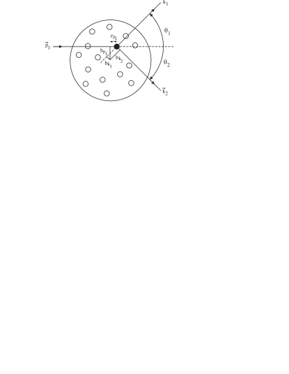
Figure 2: Geometry of the scattering process. The vectors $\vec{b}_{p_{1}}$, $\vec{b}_{k_{1}}$, and $\vec{b}_{k_{2}}$ are the impact parameters for each of the three paths for a collision occurring at $\vec{r}$. $z_{p_{1}}$, $z_{k_{1}}$, and $z_{k_{2}}$ are the $z$ coordinates of the collision point in the respective coordinate systems. $\theta_{1}$ and $\theta_{2}$ are the angles of the outgoing nucleons relative to the incoming proton direction.

It is worth remarking that the eikonal IFSI operators of Eq. (40c) are one-body operators, i.e., they do not depend on the coordinates $\left(\vec{r}_{2},\vec{r}_{3},\ldots,\vec{r}_{A}\right)$ of the residual nucleons. The normalization of the bound-state wave functions simplifies the IFSI factor (33) considerably to $\mathcal{S}_{IFSI}(\vec{r})={\widehat{\mathcal{S}}_{k1}\left(\vec{r}\right)}\>{\widehat{\mathcal{S}}_{k2}\left(\vec{r}\right)}\>{\widehat{\mathcal{S}}_{p1}\left(\vec{r}\right)}$ in the ROMEA case.

In the numerical calculations, we have employed the global $S-V$ parametrizations of Cooper et al. cooper93 and the optical potential of van Oers et al. oers82 to describe the PNPI and TRIUMF data, respectively. Hereafter, the $A(p,2p)$ calculations which adopt Eq. (40c) as a starting basis are labeled the relativistic optical model eikonal approximation (ROMEA).

II.3.3 Relativistic multiple-scattering Glauber approximation

In the ROMEA approach, all the IFSI effects are parametrized in terms of mean-field like optical potentials, i.e., the IFSI are seen as a scattering of the nucleon with the residual nucleus as a whole. As the energy increases, shorter distances are probed and the scattering with the individual nucleons becomes more relevant. For proton kinetic energies $T_{p}\geq 1$ GeV, the highly inelastic and diffractive character of the underlying elementary proton-nucleon scattering cross sections makes the Glauber approach glauber70 ; wallace75 ; yennie71 more natural. This method reestablishes the link between proton-nucleus interactions and the elementary proton-proton and proton-neutron scattering. It essentially relies on the eikonal, or, equivalently, the small-angle approximation and the assumption of consecutive cumulative scatterings of a fast nucleon on a composite target containing “frozen” point scatterers (nucleons).

In relativistic Glauber theory, the scattering wave function of a nucleon with energy $E=\sqrt{k^{2}+M^{2}}$ and spin state $\left|\frac{1}{2}m_{s}\right>$ reads debruyne02 ; ryckebusch03

$$\psi_{\vec{k},m_{s}}^{(+)}=\sqrt{\frac{E+M}{2M}}{\widehat{\mathcal{S}}}\left[\begin{array}[]{c}1\\ \frac{1}{E+M}\vec{\sigma}\cdot\hat{\vec{p}}\end{array}\right]e^{i\vec{k}\cdot\vec{r}}\chi_{\frac{1}{2}m_{s}}\;.$$ (41)

The operator ${\widehat{\mathcal{S}}}$ implements the subsequent elastic or “mildly inelastic” collisions of the fast nucleon with the “frozen” spectator nucleons

$${\widehat{\mathcal{S}}\left(\vec{r},\vec{r}_{2},\vec{r}_{3},\ldots,\vec{r}_{A}\right)}\equiv\prod_{j=2}^{A}\left[1-\Gamma\left(\vec{b}-\vec{b_{j}}\right)\theta\left(z-z_{j}\right)\right]\;,$$ (42)

where $\theta\left(z-z_{j}\right)$ ensures that the nucleon only interacts with other nucleons if they are localized in its forward propagation path. Given the diffractive nature of $pN$ collisions at GeV energies, the profile function $\Gamma\left(\vec{b}\right)$ for central elastic $pN$ scattering is parametrized in a functional form of the type

$$\Gamma\left(\vec{b}\right)=\frac{{\sigma^{tot}_{pN}}\left(1-i{\epsilon_{pN}}\right)}{4\pi\beta_{pN}^{2}}\>exp\left(-\frac{\vec{b}^{2}}{2\beta_{pN}^{2}}\right)\;.$$ (43)

At lower energies that part of the profile function proportional to $\epsilon_{pN}$ is non-Gaussian and makes significant contributions to nuclear scattering. Rather than Eq. (43) a parametrization in terms of the Arndt $NN$ phases SAID is appropriate at lower energies. For the calculations presented here, which address higher energies, the Gaussian-like real part of $\Gamma\left(\vec{b}\right)$ is the dominant contributor and the use of Eq. (43) is justified. The parameters in Eq. (43) can be determined directly from elementary nucleon-nucleon scattering experiments and include the total $pN$ cross sections $\sigma^{tot}_{pN}$, the slope parameters $\beta_{pN}$, and the ratios of the real to the imaginary part of the scattering amplitude $\epsilon_{pN}$. We obtained these Glauber parameters through interpolation of the data base available from the Particle Data Group pdg (for more details, see Ref. ryckebusch03 ). As in the ROMEA framework, only the central spin-independent contribution is retained and the impulse operator is replaced by the nucleon momentum.

The Glauber operators in Eq. (33) take the following form

$$\widehat{\mathcal{S}}_{p1}\left(\vec{r},\vec{r}_{2},\vec{r}_{3},\ldots,\vec{r}_{A}\right)=\prod_{j=2}^{A}\left[1-\Gamma\left(\vec{b}-\vec{b_{j}}\right)\theta\left(z-z_{j}\right)\right]\;,$$ (44a)

$$\widehat{\mathcal{S}}_{k1}\left(\vec{r},\vec{r}_{2},\vec{r}_{3},\ldots,\vec{r}_{A}\right)=\prod_{j=2}^{A}\left[1-\Gamma\left(\vec{b}\,^{\prime}-\vec{b_{j}}\,^{\prime}\right)\theta\left(z_{j}\,^{\prime}-z\,^{\prime}\right)\right]\;,$$ (44b)

$$\widehat{\mathcal{S}}_{k2}\left(\vec{r},\vec{r}_{2},\vec{r}_{3},\ldots,\vec{r}_{A}\right)=\prod_{j=2}^{A}\left[1-\Gamma\left(\vec{b}\,^{\prime\prime}-\vec{b_{j}}\,^{\prime\prime}\right)\theta\left(z_{j}\,^{\prime\prime}-z\,^{\prime\prime}\right)\right]\;,$$ (44c)

where $\vec{r}$ denotes the collision point and $\left(\vec{r}_{2},\vec{r}_{3},\ldots,\vec{r}_{A}\right)$ are the positions of the frozen spectator protons and neutrons in the target. The $(\vec{b},z)$, $(\vec{b}\,^{\prime},z\,^{\prime})$, and $(\vec{b}\,^{\prime\prime},z\,^{\prime\prime})$ coordinate systems are defined as in the previous section. The step functions make sure that the incoming proton can only interact with the spectator nucleons which it encounters before the “hard” collision and the outgoing protons can only interact with the spectator nucleons which they find in their forward propagation paths.

Contrary to ROMEA, the Glauber IFSI operators of Eq. (44c) are genuine $A$-body operators, so the integration over the coordinates of the spectator nucleons in Eq. (33) has to be carried out explicitly. This makes the numerical evaluation of the Glauber IFSI factor very challenging. Standard numerical integration techniques were adopted to evaluate the IFSI factor and no additional approximations, such as the commonly used thickness-function approximation, were introduced.

Henceforth, we refer to calculations based on Eq. (44c) as the relativistic multiple-scattering Glauber approximation (RMSGA).

III Numerical results for the IFSI factor

In this section, results for the IFSI factor (33) are given for the knockout of nucleons from the Fermi level in ¹²C, ¹⁶O, and ⁴⁰Ca, at an incident energy $T_{p1}=1$ GeV and a scattered proton kinetic energy $T_{k1}=870$ MeV. Thereby, we adopt coplanar scattering angles $(\theta_{1},\theta_{2})=(13.4^{\circ},67^{\circ})$ on opposite sides of the incident beam, i.e., kinematics corresponding with the PNPI experiment of Ref. belostotsky87 . All IFSI effects are included in the IFSI factor $\mathcal{S}_{IFSI}(\vec{r})$. Note that in the absence of initial- and final-state interactions the real part of the IFSI factor equals one, whereas the imaginary part vanishes identically.

The $A(p,2p)$ IFSI factor is a function of three independent variables $(r,\theta,\phi)$. The $z$-axis is chosen along the direction of the incoming beam $\vec{p}_{1}$, the $y$-axis lies along $\vec{p}_{1}\times\vec{k}_{1}$ and the $x$-axis lies in the scattering plane defined by the proton momenta $\vec{p}_{1}$ and $\vec{k}_{1}$. $\theta$ and $\phi$ denote the polar and azimuthal angles with respect to the $z$-axis and the $x$-axis, respectively. The radial coordinate $r$ represents the distance relative to the center of the target nucleus.

III.1 $\theta$ dependence

To gain a better insight into the dependence of the IFSI factor on $r$, $\theta$, and $\phi$, we calculated the contribution of the three distorting functions $\widehat{\mathcal{S}}_{p1}$, $\widehat{\mathcal{S}}_{k1}$, and $\widehat{\mathcal{S}}_{k2}$ to the IFSI factor. In Figs. 3 and 4 results are displayed for the computed real and imaginary part of $\mathcal{S}_{IFSI}(r,\theta,\phi=0)$, for proton emission from the Fermi level in ¹²C. The results were computed within the ROMEA framework, using the EDAD1 optical-potential parametrization of cooper93 .

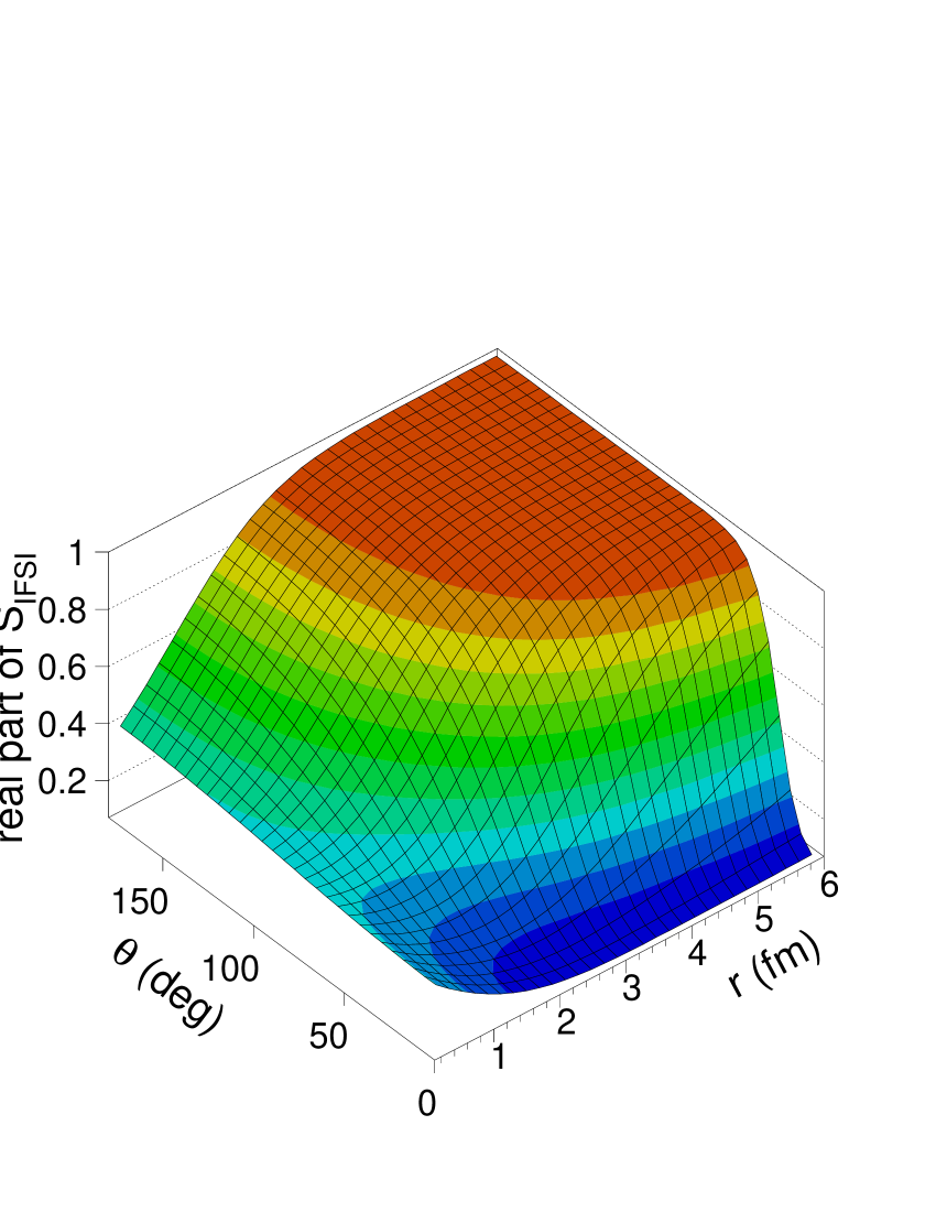
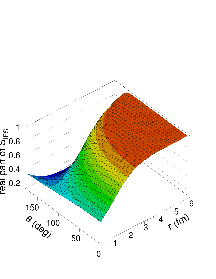
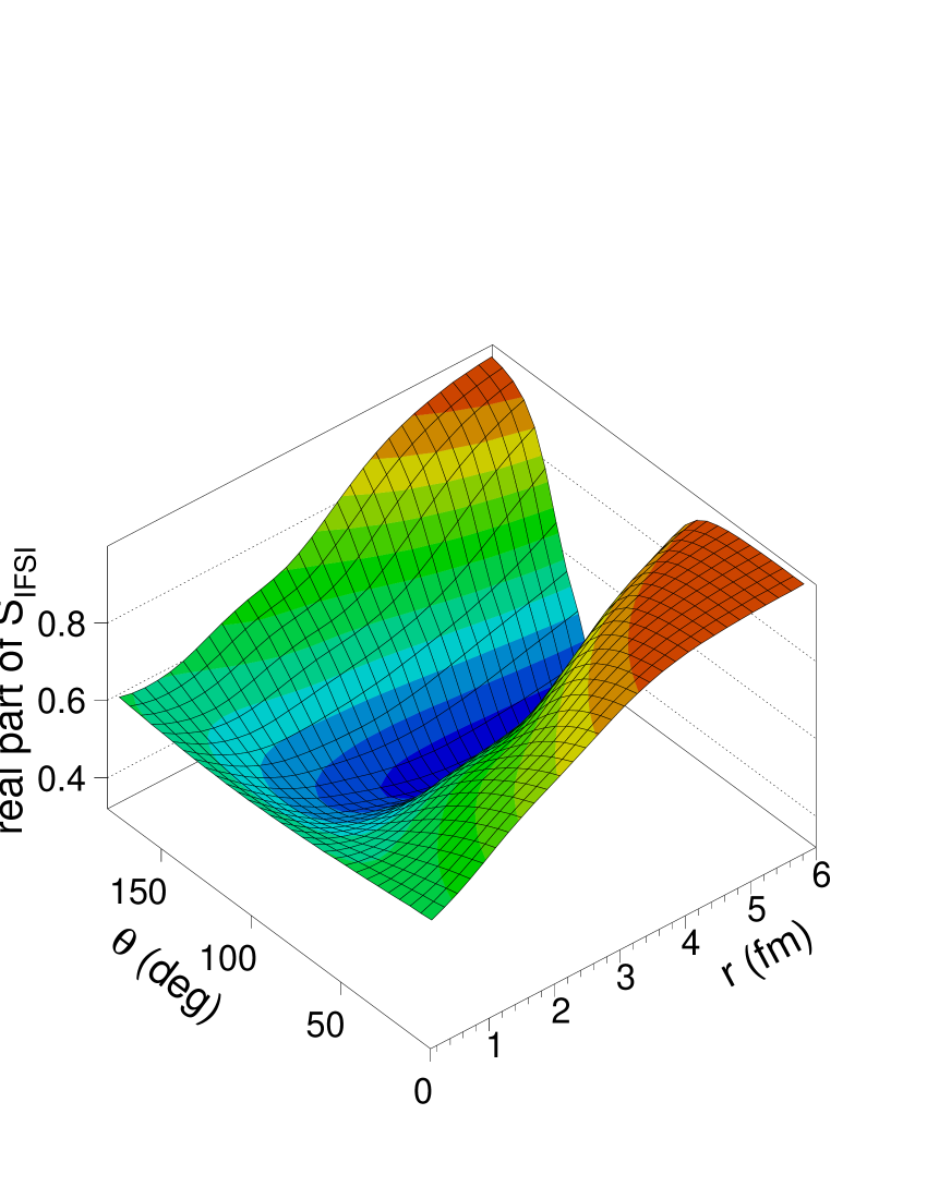
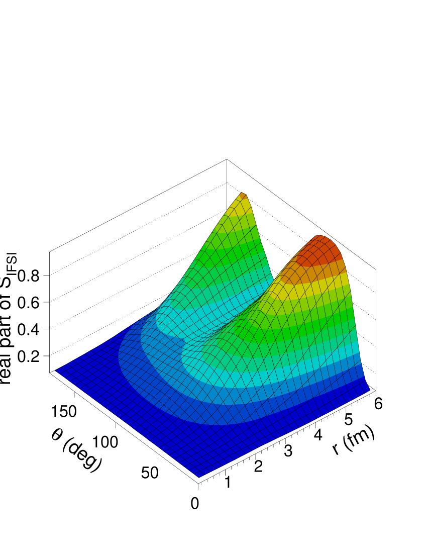
Figure 3: (Color online) The radial and polar-angle dependence of the real part of the IFSI factor $\mathcal{S}_{IFSI}$ in the scattering plane ($\phi=0^{\circ}$) for proton knockout from the Fermi level in ¹²C. The upper left panel is the contribution from the impinging proton ($\widehat{\mathcal{S}}_{p1}$), while the upper right panel shows the effect of the FSI of the scattered proton ($\widehat{\mathcal{S}}_{k1}$). In the bottom left figure, the effect of the FSI of the ejected proton ($\widehat{\mathcal{S}}_{k2}$) is presented and the bottom right figure shows the complete IFSI factor ($\widehat{\mathcal{S}}_{k1}\>\widehat{\mathcal{S}}_{k2}\>\widehat{\mathcal{S}}_{p1}$). The kinematics was $T_{p1}=1$ GeV, $T_{k1}=870$ MeV, $\theta_{1}=13.4^{\circ}$, and $\theta_{2}=67^{\circ}$.

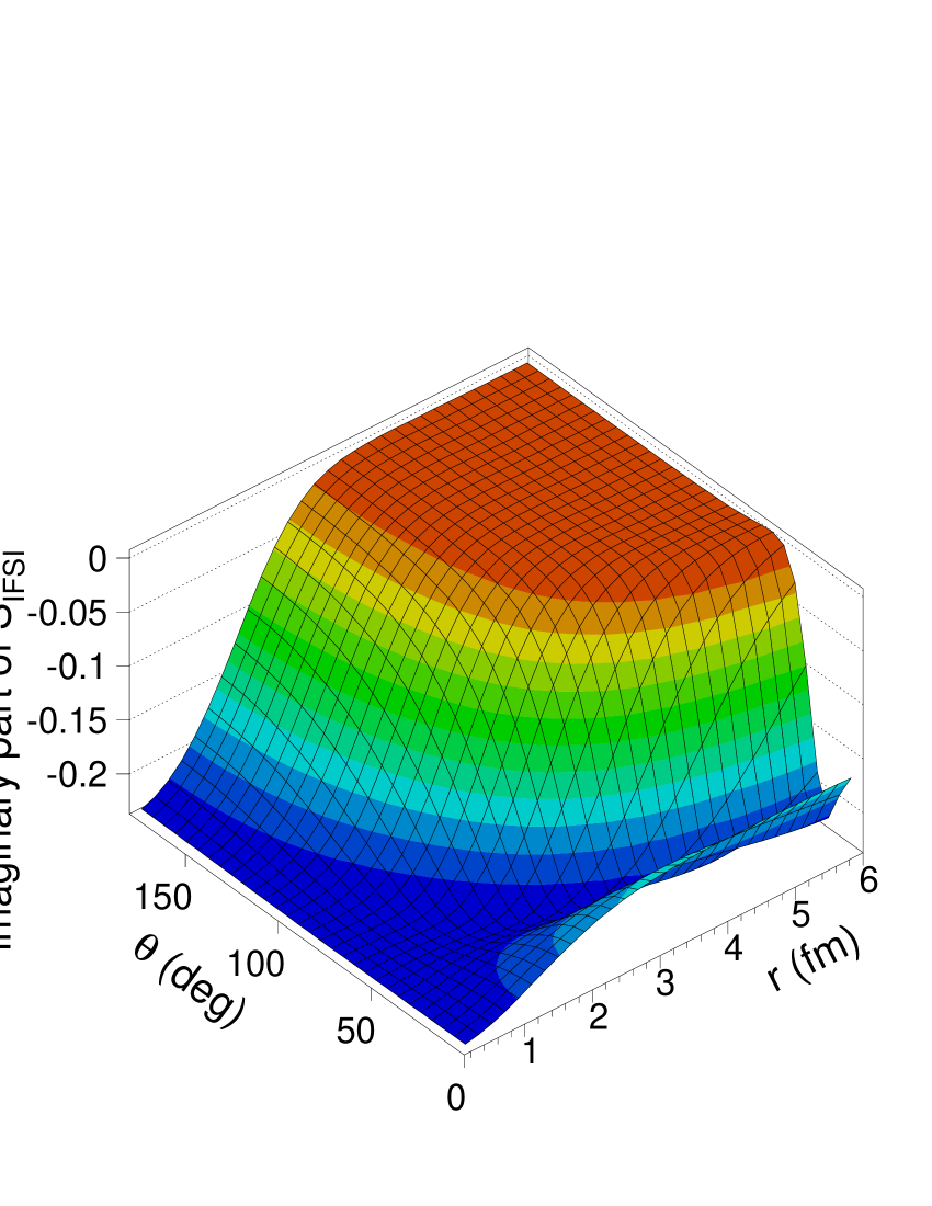
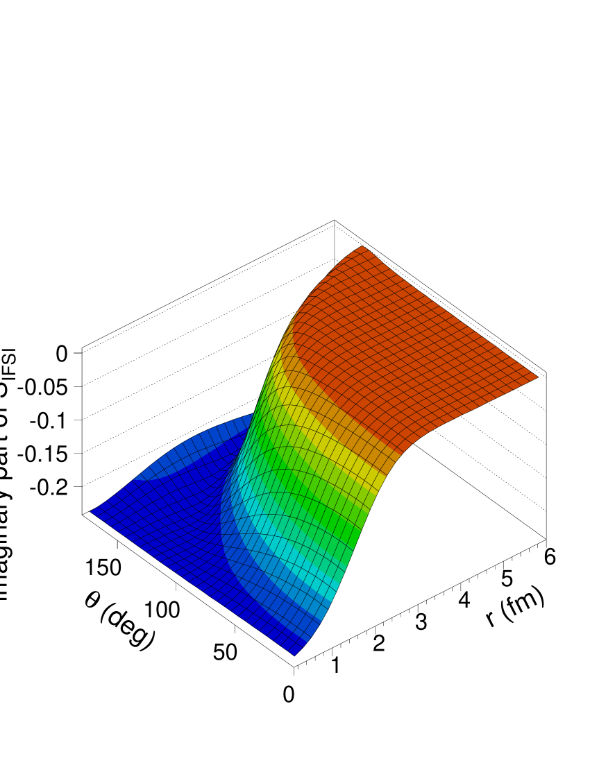
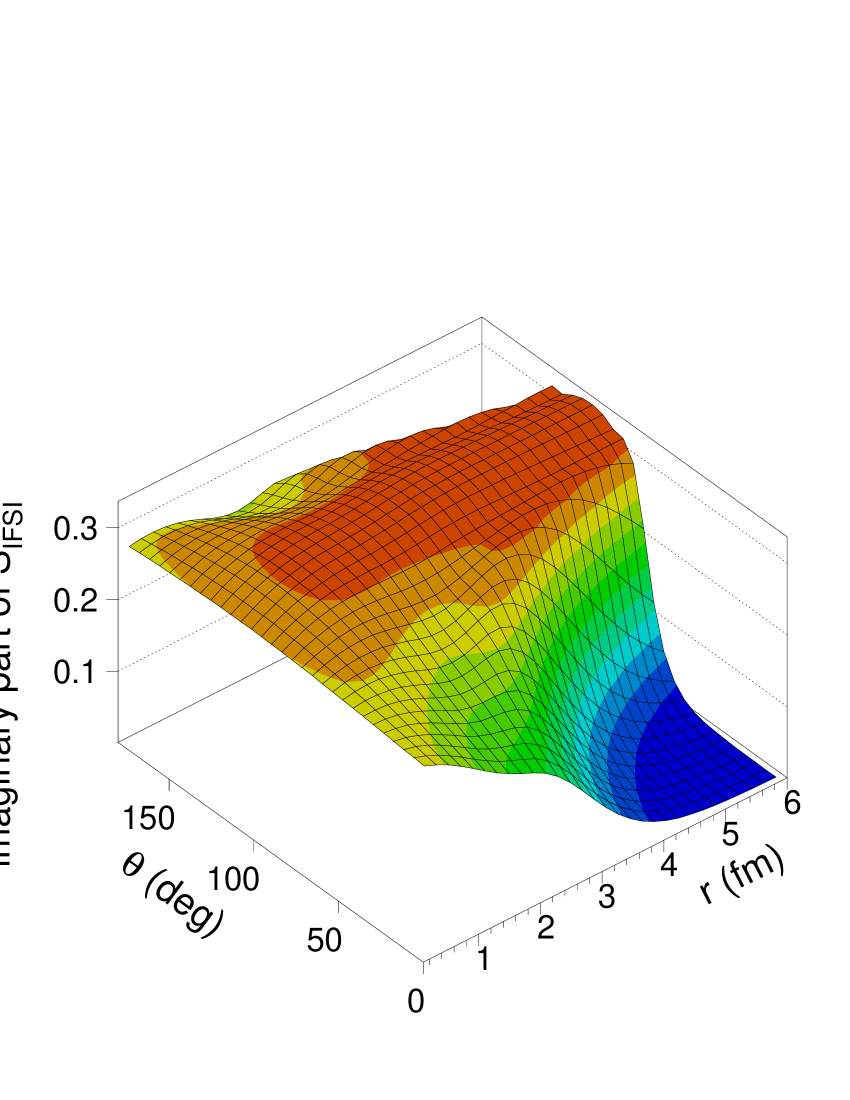
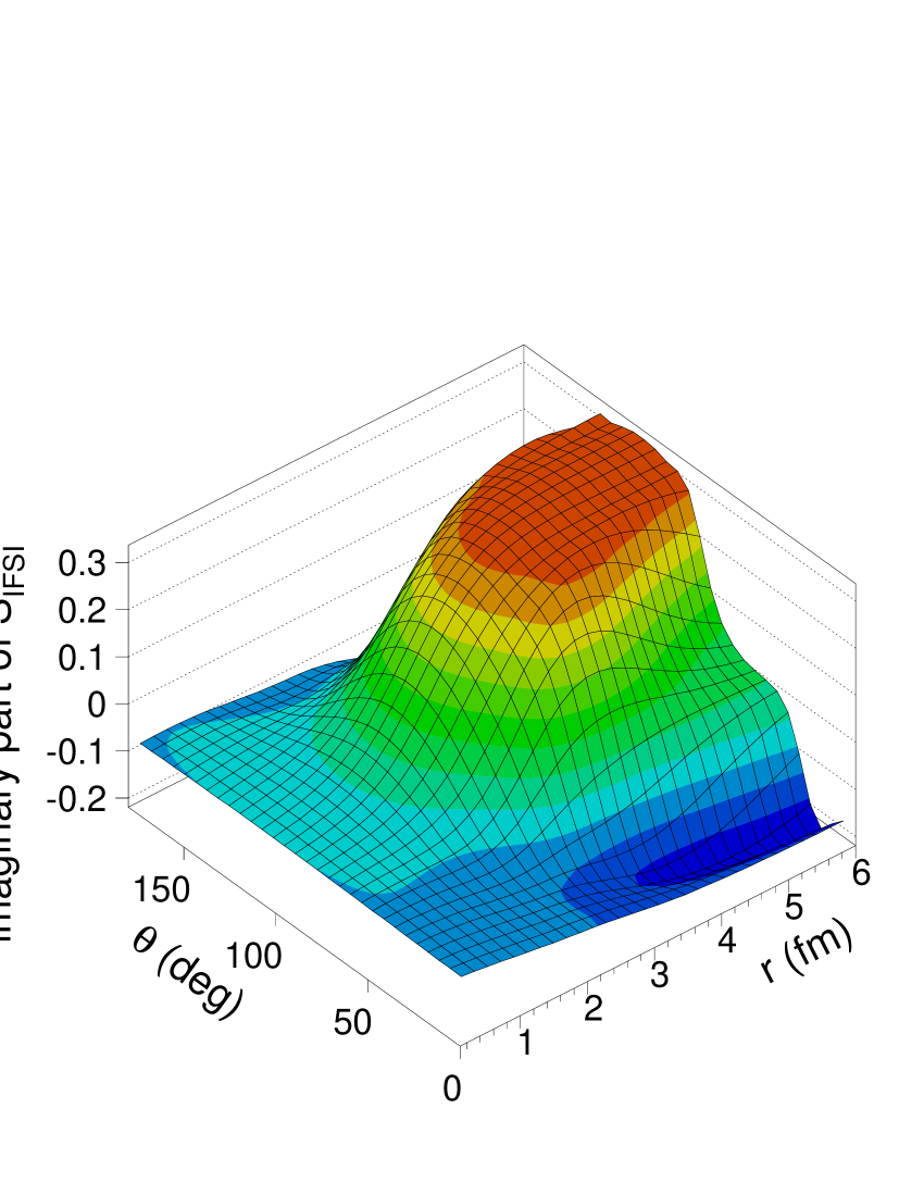
Figure 4: (Color online) As in Fig. 3 but now for the imaginary part of the IFSI factor.

The $\theta$ dependence can be interpreted as follows. For a given $r$, the distance that the incoming proton travels through the target nucleus before colliding “hard” with a target nucleon, decreases with increasing angle $\theta$. As a consequence, small values of $\theta$ induce the largest ISI. For the FSI of the scattered proton, the opposite holds true and $\theta=180^{\circ}$ for a large $r$ value corresponds to an event whereby the “hard” collision transpires at the outskirts of the nucleus and the scattered proton has to travel through the whole nucleus before it becomes asymptotically free, thus giving rise to the smallest (largest) values for the real (imaginary) part of the IFSI factor. Unlike the scattered proton, which moves almost collinear to the $z$-axis, the ejected nucleon leaves the nucleus under a large scattering angle $\theta_{2}$. Hence, the FSI are minimal for $\theta$ close to $0^{\circ}$ or $180^{\circ}$ and maximal for $\theta$ around $180^{\circ}-\theta_{2}$. Finally, the $\theta$ dependence of the complete IFSI factor is the result of the interplay between the three distorting effects, with the strongest scattering and absorption observed at $\theta$ close to $0^{\circ}$, $180^{\circ}-\theta_{2}$, and $180^{\circ}$.

III.2 $r$ dependence

Figure 5 displays the real part of the IFSI factor as a function of $r$ at various values of $\theta$. The ROMEA calculations were performed for the same kinematics as in Figs. 3 and 4, and use the EDAI optical-potential fit of cooper93 .

Figure 5: The radial dependence of the real part of the IFSI factor $\mathcal{S}_{IFSI}$ in the scattering plane ($\phi=0^{\circ}$) for neutron knockout from the Fermi level in ⁴⁰Ca. The upper left, upper right, and bottom left panels display $\widehat{\mathcal{S}}_{p1}$, $\widehat{\mathcal{S}}_{k1}$, and $\widehat{\mathcal{S}}_{k2}$, respectively, while the complete IFSI factor is shown in the bottom right picture.

Turning first to the upper left panel, it can be inferred from the picture that the ISI effects increase with growing $r$ for $\theta=0^{\circ}$. For $\theta=45^{\circ}$ and increasing $r$, initially, the growing distance the proton has to travel through the nucleus leads to a decrease of the real part of $\widehat{\mathcal{S}}_{p1}$. This is followed by an increase for larger $r$ up to $\widehat{\mathcal{S}}_{p1}=1$. This reduction in ISI effects with increasing $r$ is brought about by the incoming proton’s path through the nucleus moving away from the nuclear interior and closer to the less dense nuclear surface. The other curves of the upper left figure illustrate a general trend for $90^{\circ}\leq\theta\leq 180^{\circ}$ : as $r$ increases, the real part of the IFSI factor grows correspondingly. As can be appreciated from Fig. 5 as well as from the previous figures, the global behavior of the $\widehat{\mathcal{S}}_{k1}$ factor describing the scattered proton’s FSI can be related to that of the ISI factor $\widehat{\mathcal{S}}_{p1}$ through the substitution $\theta\rightarrow 180^{\circ}-\theta$. This approximate symmetry can be attributed to the small scattering angle $\theta_{1}$, i.e., the scattered proton leaves the nucleus almost parallel to the incoming proton’s direction. In the bottom left panel, the additional curve ($\theta=115^{\circ}$, i.e., close to $180^{\circ}-\theta_{2}$) represents the situation of maximal FSI of the ejected nucleon. For this $\theta$ value, the path of the ejected nucleon passes through the center of the nucleus and the distance travelled through the nucleus increases with $r$. Accordingly, the real part of $\widehat{\mathcal{S}}_{k2}$ is a monotonously decreasing function of $r$. The other extreme is the $\theta=0^{\circ}$ case where increasing $r$ means less FSI. For the other $\theta$ values, the absorption reaches its maximum for some intermediate $r$ value. Again, the combination of $\widehat{\mathcal{S}}_{p1}$, $\widehat{\mathcal{S}}_{k1}$, and $\widehat{\mathcal{S}}_{k2}$ determines the total IFSI factor with the strongest attenuation predicted in the nuclear interior.

III.3 $\phi$ dependence

The dependence of the IFSI factor on the azimuthal angle of the collision point is quite straightforward. One representative result is displayed in Fig. 6. Here, $\cos\phi\geq 0$ ($\cos\phi\leq 0$) refers to a situation where the “hard” $NN$ collision occurs in the upper (lower) hemisphere with respect to the $yz$-plane (see Fig. 2 for a collision point located in the upper hemisphere). Due to the cylindrical symmetry about the $z$-axis, the factor describing the ISI of the incoming proton is independent of $\phi$. Regarding the scattered proton, we observe the least FSI in the upper hemisphere, since the proton then avoids passing through the highly absorbing nuclear interior. For the ejected nucleon, the contrary applies and the strongest FSI effects are found for $\phi=0^{\circ}$. As the $xz$-plane is defined as the scattering plane, the IFSI factor possesses the symmetry $\mathcal{S}_{IFSI}(r,\theta,2\pi-\phi)=\mathcal{S}_{IFSI}(r,\theta,\phi)$ for coplanar scattering.

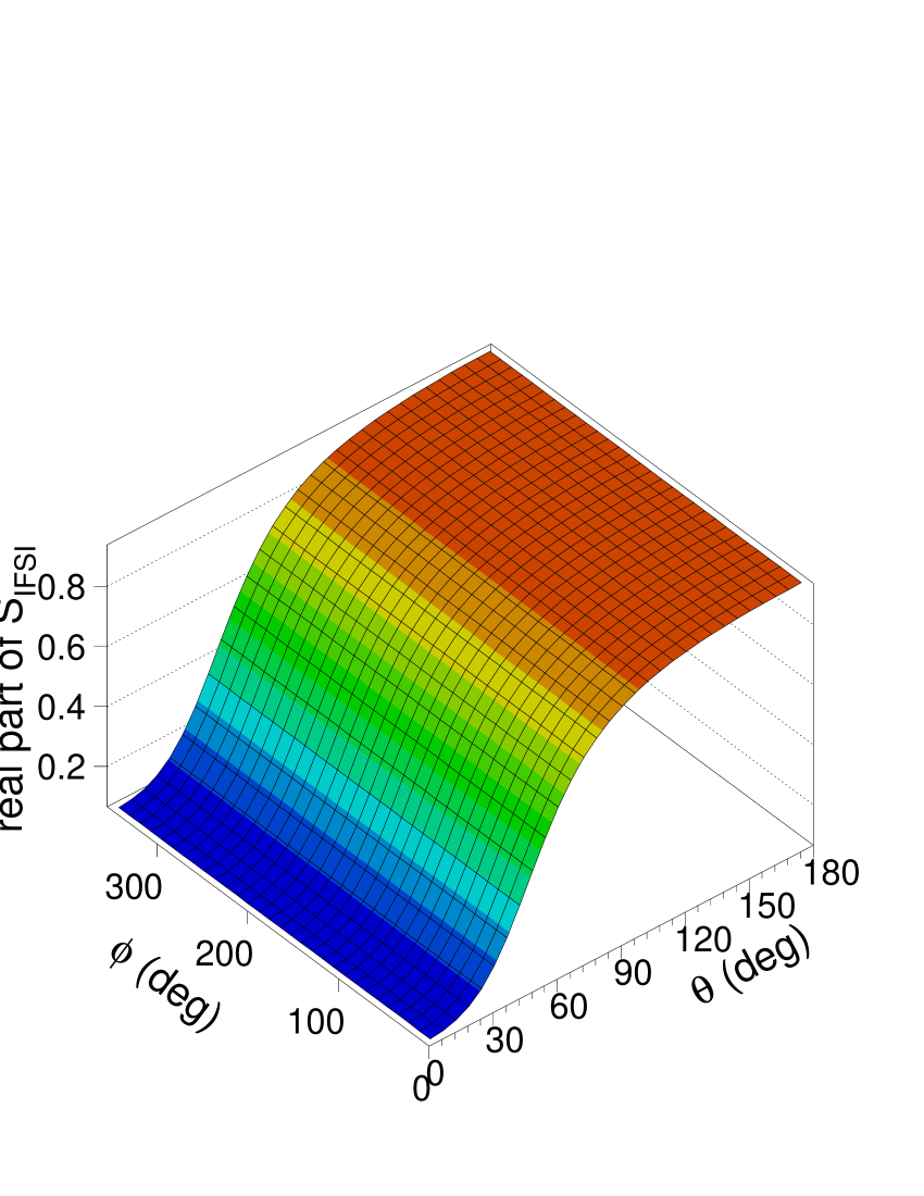
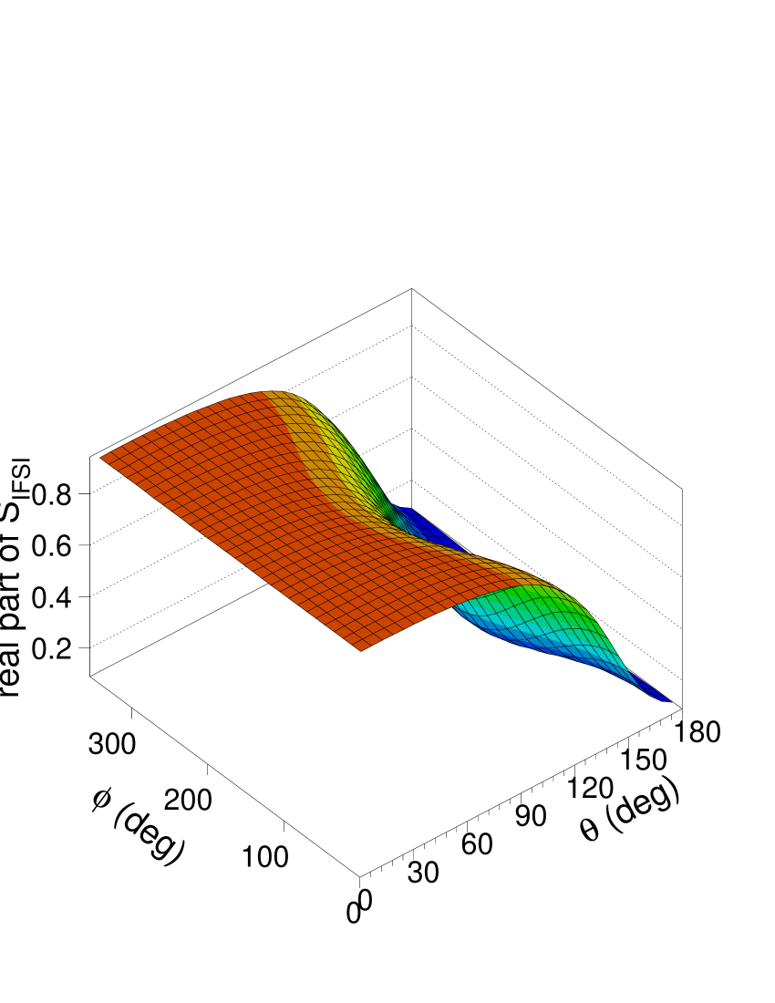
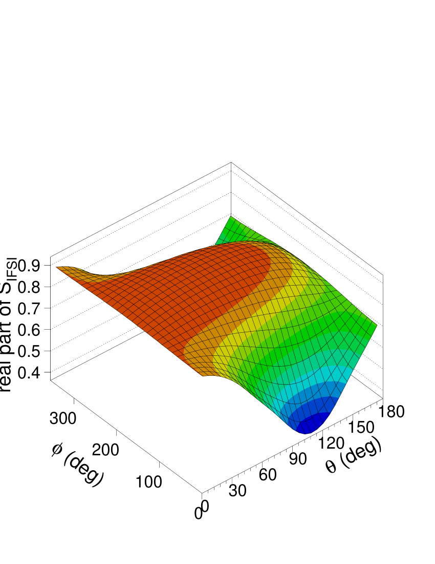
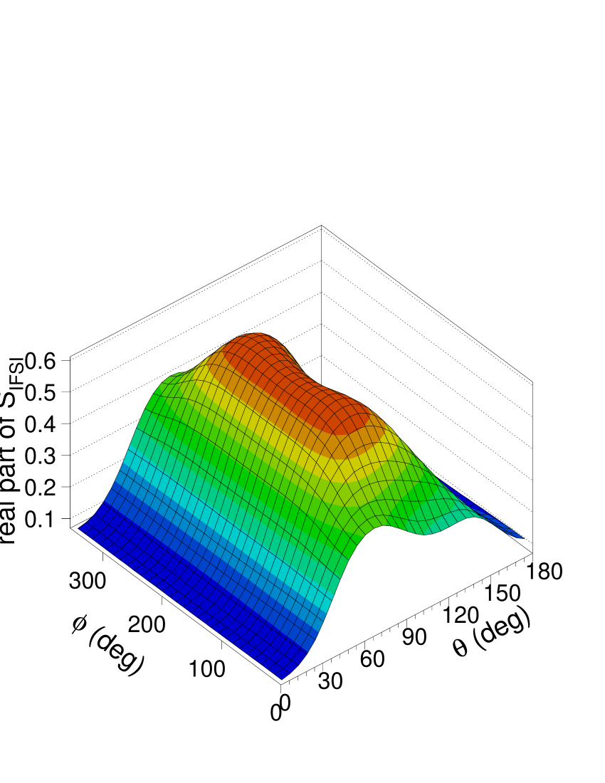
Figure 6: (Color online) The polar- and azimuthal-angle dependence of the real part of $\mathcal{S}_{IFSI}(r=3~{}fm,\theta,\phi)$ for proton knockout from the Fermi level in ¹⁶O. Kinematics as in Fig. 3. ROMEA calculation with the EDAD2 optical potential cooper93 . As in the previous figures, the upper left, upper right, and bottom left panels represent the effect of the ISI of the incoming proton, the FSI of the scattered proton, and the FSI of the struck nucleon, respectively, whereas the bottom right figure displays the complete IFSI factor.

III.4 Level and $A$ dependence

Results for the emission from levels other than the Fermi level have not been plotted here, as it turns out that the IFSI factors hardly depend on the single-particle level in which the struck nucleon resides. The peculiar spatial characteristics of the different single-particle orbits have an impact on the observables, though. Indeed, the distorted momentum-space wave function $\phi_{\alpha_{1}}^{D}$ of Eq. (32) is determined by the values of the IFSI factor folded with a relativistic bound-state wave function $\phi_{\alpha_{1}}\left(\vec{r}\right)$. As the particles experience less IFSI close to the nuclear surface, one obtains a stronger reduction of the quasifree cross section for nucleon knockout from a level which has a larger fraction of its density in the nuclear interior. This will become apparent in Fig. 7, but even more so in Sec. IV.1.

Figure 7 shows a function $\delta\left(r\right)$ which represents the contribution of the nuclear region with radial coordinate $r$ to the differential cross section. The procedure to calculate this function is similar to the method exposed in Ref. hatanaka97 and is developed in Appendix B. Comparison of the upper and lower panels illustrates that IFSI mechanisms make the $A(p,2p)$ cross sections reflect surface mechanisms, unlike the $A(e,e^{\prime}p)$ reaction where the weakly interacting electron probes the entire nuclear volume and only the outgoing proton interacts with the residual system. Apart from the shift to higher $r$, the IFSI brings about a strong reduction in the magnitude of the cross sections, whereby the Fermi level is least affected. Even though $\delta\left(r\right)$ is concentrated in the surface region, the average density seen through this reaction still amounts to $0.069$ fm^-3 ($0.080$ fm^-3) or $32\%$ ($45\%$) of the central density in the case of $1s_{1/2}$ knockout from ¹²C (⁴⁰Ca). In the case of emission from the Fermi level, on the other hand, the average density is only $12\%$ ($13\%$) of the central density for a ¹²C (⁴⁰Ca) target.

Figure 7: Contribution to the $A(p,2p)$ cross section $\delta\left(r\right)$ as a function of $r$. The upper figures present the results obtained after setting the IFSI factor $\mathcal{S}_{IFSI}(\vec{r})$ equal to one in Eq. (B), whereas in the lower panels the ROMEA calculations using the EDAD1 optical potential are depicted. The dashed (dot-dashed) curves show the result for emission from the Fermi (lowest-lying $1s_{1/2}$) level. The baryon density $\rho\left(r\right)$ is also shown (solid curve). The ordinate is given for $\rho\left(r\right)$. The $\delta\left(r\right)$ are plotted in units of fm² up to an arbitrary scaling factor. The kinematics was $T_{p1}=1$ GeV, $T_{k1}=870$ MeV, $\theta_{1}=13.4^{\circ}$, and $\theta_{2}=67^{\circ}$.

Also, the IFSI factors for neutron emission are almost identical to the corresponding IFSI factors for proton knockout and, as expected, the overall effect of IFSI is more pronounced for heavier target nuclei.

III.5 Comparison between ROMEA and RMSGA calculations

In this subsection, we investigate the sensitivity of the computed IFSI factors to the adopted parametrizations for the optical potentials and compare the ROMEA results with the RMSGA predictions. As can be seen in Fig. 8, the IFSI factor depends on whether $A$-dependent (EDAD1/EDAD2) or $A$-independent (EDAI) fits for the potentials are selected, but the global features are comparable. Figure 9, as contrasted to Fig. 3, demonstrates that the RMSGA method adequately describes the ISI of the incoming proton and the FSI of the scattered proton. However, the discrepancies between ROMEA and RMSGA become significant in the calculation of the FSI of the ejected nucleon (note the different scales in the bottom left panels of Figs. 3 and 9), and therefore also in the complete IFSI factor. The noted difference is attributed to the low ejectile kinetic energy ($T_{k2}\approx 114$ MeV for the specific case of Fig. 9, and comparable values for knockout from other levels and other nuclei). At such low energies, the RMSGA predictions are not realistic due to the underlying approximations, mostly the postulation of linear trajectories and frozen spectator nucleons. So, for the kinematics discussed here, the ROMEA method is to be preferred over the RMSGA one, as the latter overestimates the distortion for the low-energetic ejectile nucleon.

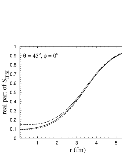
Figure 8: The sensitivity of the real part of the complete IFSI factor for neutron knockout from ¹²C to the adopted choice for the parametrization of the optical potentials. Results of ROMEA calculations with the EDAD1 (solid curve), EDAD2 (dashed curve), and EDAI (dot-dashed curve) optical potentials are shown. Kinematics as in Fig. 3.

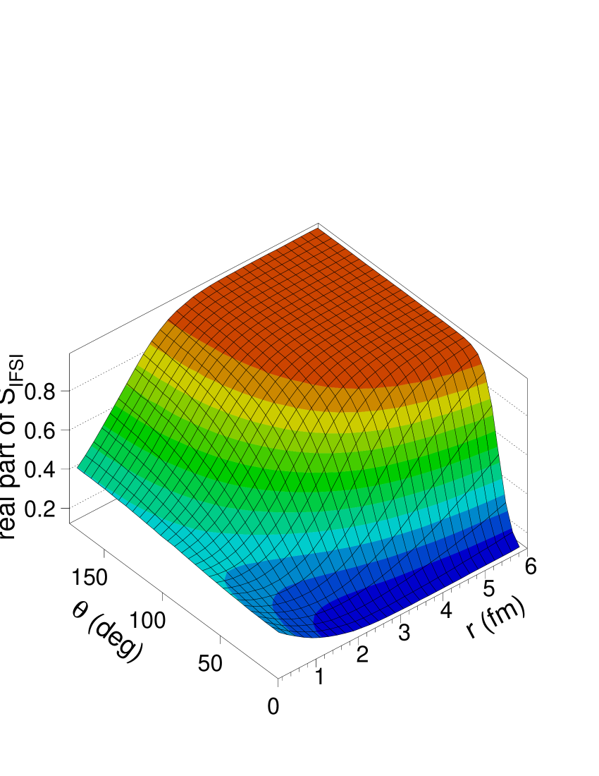
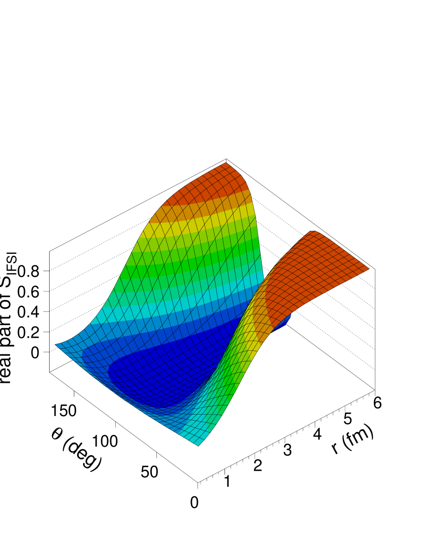
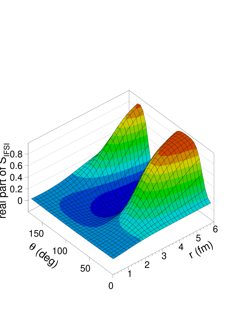
Figure 9: (Color online) As in Fig. 3 but now using the RMSGA method.

IV Numerical results for $A(p,pN)$ differential cross sections

IV.1 The PNPI experiment

The PNPI experiment belostotsky87 was carried out with an incident proton beam of energy $1$ GeV. The scattered proton was detected at $\theta_{1}=13.4^{\circ}$ with a kinetic energy between $800$ and $950$ MeV, while the knocked-out nucleon was observed at $\theta_{2}=67^{\circ}$ having a kinetic energy below $200$ MeV.

Figures 10–12 display a selection of differential cross section results as a function of the kinetic energy of the most energetic nucleon in the final state. The EDAI optical potential cooper93 was used for the ROMEA calculations. The other parametrizations of Ref. cooper93 produce similar predictions, whereas the RMSGA approach fails to give an adequate description of the data because of the low kinetic energy of the ejected nucleon. Since the experiment of Ref. belostotsky87 only measured relative cross sections, the ROMEA results were normalized to the experimental data.

Figure 10: Differential cross section for the ¹²C$(p,2p)$ reaction. The solid curve represents the ROMEA calculation, whereas the dashed curve is the plane wave result reduced by the indicated factor. The ROMEA results are normalized to the data. Data points are from Ref. belostotsky87 . The magnitude of the experimental error bars is estimated to be of the order of $5$–$10\%$.

Figure 11: As in Fig. 10 but for the ¹⁶O$(p,pn)$ reaction.

Figure 12: As in Fig. 10 but for the ⁴⁰Ca$(p,pn)$ reaction.

The ROMEA calculations reproduce the shapes of the measured differential cross sections. Furthermore, comparison of the RPWIA and ROMEA calculations shows that the effect of the IFSI is twofold. First, IFSI result in a reduction of the RPWIA cross section that is both level and $A$ dependent. From the figures it is clear that ejection of a nucleon from a deeper lying level leads to stronger initial- and final-state distortions. This reflects the fact that the incoming and outgoing nucleons encounter more obstacles when a deeper lying bound nucleon is probed. The $A$ dependence also conforms with our expectations, i.e., the IFSI effects are larger for heavier nuclei. Besides the attenuation, the IFSI also make the measured missing momentum different from the initial momentum of the struck nucleon. As can be inferred from Fig. 13, this momentum shift leads to an asymmetry between the positive and negative missing-momentum side of the momentum distribution. Note that positive missing momentum corresponds to $p_{m_{x}}=k_{1}\sin\theta_{1}+k_{2}\sin\theta_{2}\cos\phi_{2}>0$.

Figure 13: The ¹²C$(p,2p)$ momentum distribution for the $1p_{3/2}$ state as a function of the missing momentum. The solid (dashed) curve are ROMEA (RPWIA) calculations.

IV.2 The TRIUMF ⁴He$(p,2p)$ experiment

Finally, we present some results for the ⁴He$(p,2p)$ reaction at an incident proton energy of $250$ MeV. Figure 14 compares the data from the TRIUMF experiment oers82 with ROMEA calculations using the optical potential of van Oers et al. oers82 . The typical shape for knockout of an $s$-state proton is reproduced by the ROMEA predictions. This fair agreement of the ROMEA results with the data demonstrates that our ROMEA model also works satisfactorily at lower incident energies.

Figure 14: Differential cross section for the ⁴He$(p,2p)$ reaction at the angle pairs $(40^{\circ},40^{\circ})$ and $(45^{\circ},35^{\circ})$ at $250$ MeV. The solid (dashed) curves refer to ROMEA (RPWIA) results. The data are from Ref. oers82 .

V Conclusions

A relativistic and cross-section factorized framework to describe the IFSI in quasielastic $A(p,pN)$ reactions has been outlined. The model, which relies on the eikonal approximation, can use either optical potentials or Glauber multiple-scattering theory to deal with IFSI. Thanks to the freedom of choice between these two substantially different techniques, our model is expected to be applicable at both intermediate and high incident energies.

The properties of the IFSI factor have been investigated for an incident proton energy of $1$ GeV. Not surprisingly, the strongest attenuation occurs in the nuclear interior and heavier target nuclei are found to induce larger IFSI effects. Also, the surface-peaked character of the $A(p,pN)$ reaction was clearly established to be a consequence of the IFSI. Whereas the different types of optical-potential sets contained in Ref. cooper93 yield comparable IFSI factors, the RMSGA calculations exhibit an unrealistic behavior for these kinematics.

The ROMEA model has been used to calculate cross sections for the kinematics of two different experiments : quasielastic proton scattering from ¹²C, ¹⁶O, and ⁴⁰Ca at $1$ GeV, and ⁴He$(p,2p)$ scattering at $250$ MeV. The predictions are shown to reproduce the shape of the data reasonably well at both incoming energies, thereby providing support for the wide applicability range of our model.

Although the RMSGA approach was deemed unsuitable for the kinematics discussed here, it should prove useful when trying to describe nuclear transparency data. Work in this direction is in progress.

Appendix A Relativistic bound-state wave functions

For spherically symmetric potentials, the solutions $\phi_{\alpha}\left(\vec{r}\right)$ to a single-particle Dirac equation have the form Walecka2001

$$\phi_{\alpha}\left(\vec{r},\vec{\sigma}\right)\equiv\phi_{n\kappa m}\left(\vec{r},\vec{\sigma}\right)=\left[\begin{array}[]{c}i\frac{G_{n\kappa}(r)}{r}\;{\cal Y}_{\kappa m}(\Omega,\vec{\sigma})\\ -\frac{F_{n\kappa}(r)}{r}\;{\cal Y}_{-\kappa m}(\Omega,\vec{\sigma})\end{array}\right]\;,$$ (45)

where $n$ denotes the principal, $\kappa$ and $m$ the generalized angular momentum quantum numbers. The ${\cal Y}_{\pm\kappa m}$ are the spin spherical harmonics and determine the angular and spin parts of the wave function,

$${\cal Y}_{\kappa m}(\Omega,\vec{\sigma})=\sum_{m_{l}m_{s}}\left<lm_{l}\frac{1}{2}m_{s}\mid jm\right>Y_{lm_{l}}(\Omega)\chi_{\frac{1}{2}m_{s}}(\vec{\sigma})\;,$$

$${\cal Y}_{-\kappa m}(\Omega,\vec{\sigma})=\sum_{m_{l}m_{s}}\left<\bar{l}m_{l}\frac{1}{2}m_{s}\mid jm\right>Y_{\bar{l}m_{l}}(\Omega)\chi_{\frac{1}{2}m_{s}}(\vec{\sigma})\;,$$ (46)

with

$$j=|\kappa|-\frac{1}{2}\;,\hskip 22.76228ptl=\left\{\begin{array}[]{ll}\kappa,&\kappa>0\\ -(\kappa+1),&\kappa<0\end{array}\right.\;,\hskip 22.76228pt\bar{l}=2j-l=\left\{\begin{array}[]{ll}\kappa-1,&\kappa>0\\ -\kappa,&\kappa<0\end{array}\right.\;.$$ (47)

The Fourier transform of the relativistic bound-nucleon wave function is given by

$$\phi_{\alpha}\left(\vec{p}\right)=\int d\vec{r}e^{-i\vec{p}\cdot\vec{r}}\phi_{\alpha}\left(\vec{r}\right)=\left(-i\right)^{l}(2\pi)^{3/2}\left[\begin{array}[]{c}g_{n\kappa}(p)\;{\cal Y}_{\kappa m}(\Omega_{p})\\ -S_{\kappa}\;f_{n\kappa}(p)\;{\cal Y}_{-\kappa m}(\Omega_{p})\end{array}\right]\;,$$ (48)

with $S_{\kappa}=\kappa/\left|\kappa\right|$. The radial functions $g_{n\kappa}$ and $f_{n\kappa}$ in momentum space are obtained from their counterparts in coordinate space :

$$g_{n\kappa}(p)=i\;\sqrt{\frac{2}{\pi}}\int_{0}^{\infty}r^{2}dr\;\frac{G_{n\kappa}(r)}{r}j_{l}(pr)\;,$$ (49a)

$$f_{n\kappa}(p)=i\;\sqrt{\frac{2}{\pi}}\int_{0}^{\infty}r^{2}dr\;\frac{F_{n\kappa}(r)}{r}j_{\bar{l}}(pr)\;,$$ (49b)

with $j_{l}(pr)$ the spherical Bessel function of the first kind.

Appendix B Radial contribution to the $A(p,pN)$ cross section

The differential $A(p,pN)$ cross section (37) is proportional to the distorted momentum distribution $\rho^{D}$ of Eq. (35). When approximating the completeness relation (17) as

$$\sum_{s}u(\vec{p}_{m},s)\bar{u}(\vec{p}_{m},s)\approx 1\;,$$ (50)

i.e., neglecting the negative-energy term as in Sec. II.2, this amounts to

$$\left(\frac{d^{5}\sigma}{dE_{k1}d\Omega_{1}d\Omega_{2}}\right)^{D}\propto\sum_{m}\overline{\phi_{\alpha_{1}}^{D}}\>\phi_{\alpha_{1}}^{D}\;.$$ (51)

Thus, with $D\left(r\right)$ defined as

$$D\left(r\right)\equiv\int d\Omega\>r^{2}\>e^{-i\vec{p}_{m}\cdot\vec{r}}\>\phi_{\alpha_{1}}\left(\vec{r}\right)\>\mathcal{S}_{IFSI}\left(\vec{r}\right)\;,$$ (52)

the function

$$\delta\left(r_{1}\right) \equiv \sum_{m}\frac{1}{\Delta R}\Biggl{[}\int_{0}^{\infty}dr\>\overline{D}\left(r\right)\int_{0}^{\infty}dr\>D\left(r\right)-\Biggr{.}$$

$$\Biggl{.}\Bigl{(}\int_{0}^{r_{1}}dr\>\overline{D}\left(r\right)+\int_{r_{1}+\Delta R}^{\infty}dr\>\overline{D}\left(r\right)\Bigr{)}\Bigl{(}\int_{0}^{r_{1}}dr\>D\left(r\right)+\int_{r_{1}+\Delta R}^{\infty}dr\>D\left(r\right)\Bigr{)}\Biggr{]}$$

$$= \sum_{m}\bigl{(}\overline{D}\left(r_{1}\right)\>\phi_{\alpha_{1}}^{D}+\overline{\phi_{\alpha_{1}}^{D}}\>D\left(r_{1}\right)\bigr{)}$$

represents the contribution of an infinitesimal interval in $r$ around $r_{1}$ to the $A(p,pN)$ cross section. This procedure also enables us to estimate the average density seen through this reaction as

$$\overline{\rho}\equiv\frac{\int_{0}^{\infty}\rho\left(r\right)\>\delta\left(r\right)\>dr}{\int_{0}^{\infty}\delta\left(r\right)\>dr}\;.$$ (54)

References

- (1) G. Jacob and Th. A. J. Maris, Rev. Mod. Phys. 38, 121 (1966).
- (2) G. Jacob and Th. A. J. Maris, Rev. Mod. Phys. 45, 6 (1973).
- (3) P. Kitching, W. J. McDonald, Th. A. J. Maris, and C. A. Z. Vasconcellos, Adv. Nucl. Phys. 15, 43 (1985).
- (4) N. S. Chant and P. G. Roos, Phys. Rev. C 15, 57 (1977).
- (5) S. Kullander, F. Lemeilleur, P. U. Renberg, G. Landaud, J. Yonnet, B. Fagerström, A. Johansson, and G. Tibell, Nucl. Phys. A173, 357 (1971).
- (6) R. K. Bhowmik, C. C. Chang, P. G. Roos, and H. D. Holmgren, Nucl. Phys. A226, 365 (1974).
- (7) R. Bengtsson, T. Berggren, and Ch. Gustafsson, Phys. Rep. 41, 191 (1978).
- (8) P. Kitching, C. A. Miller, W. C. Olsen, D. A. Hutcheon, W. J. McDonald, and A. W. Stetz, Nucl. Phys. A340, 423 (1980).
- (9) W. T. H. van Oers, B. T. Murdoch, B. K. S. Koene, D. K. Hasell, R. Abegg, D. J. Margaziotis, M. B. Epstein, G. A. Moss, L. G. Greeniaus, J. M. Greben, J. M. Cameron, J. G. Rogers, and A. W. Stetz, Phys. Rev. C 25, 390 (1982).
- (10) D. S. Carman, L. C. Bland, N. S. Chant, T. Gu, G. M. Huber, J. Huffman, A. Klyachko, B. C. Markham, P. G. Roos, P. Schwandt, and K. Solberg, Phys. Lett. B452, 8 (1999).
- (11) N. S. Chant and P. G. Roos, Phys. Rev. C 27, 1060 (1983).
- (12) R. A. Arndt, I. I. Strakovsky, and R. L. Workman, Phys. Rev. C 62, 034005 (2000); Scattering Analysis Interactive Dial-in Program (SAID), http://gwdac.phys.gwu.edu/.
- (13) J. A. McNeil, L. Ray, and S. J. Wallace, Phys. Rev. C 27, 2123 (1983); J. A. McNeil, J. R. Shepard, and S. J. Wallace, Phys. Rev. Lett. 50, 1439 (1983); J. R. Shepard, J. A. McNeil, and S. J. Wallace, ibid. 50, 1443 (1983).
- (14) C. J. Horowitz, Phys. Rev. C 31, 1340 (1985); C. J. Horowitz and M. J. Iqbal, ibid. 33, 2059 (1986); D. P. Murdock and C. J. Horowitz, ibid. 35, 1442 (1987); C. J. Horowitz and D. P. Murdock, ibid. 37, 2032 (1988).
- (15) O. V. Maxwell, Nucl. Phys. A600, 509 (1996); A638, 747 (1998); O. V. Maxwell and E. D. Cooper, ibid. A656, 231 (1999).
- (16) E. D. Cooper and O. V. Maxwell, Nucl. Phys. A493, 468 (1989); O. V. Maxwell and E. D. Cooper, ibid. A513, 584 (1990); A565, 740 (1993); A574, 819 (1994); A603, 441 (1996).
- (17) Y. Ikebata, Phys. Rev. C 52, 890 (1995).
- (18) J. Mano and Y. Kudo, Prog. Theor. Phys. 100, 91 (1998).
- (19) C. A. Miller, K. H. Hicks, R. Abegg, M. Ahmad, N. S. Chant, D. Frekers, P. W. Green, L. G. Greeniaus, D. A. Hutcheon, P. Kitching, D. J. Mack, W. J. McDonald, W. C. Olsen, R. Schubank, P. G. Roos, and Y. Ye, Phys. Rev. C 57, 1756 (1998).
- (20) R. Neveling, A. A. Cowley, G. F. Steyn, S. V. Förtsch, G. C. Hillhouse, J. Mano, and S. M. Wyngaardt, Phys. Rev. C 66, 034602 (2002).
- (21) D. L. Adams and M. Bleszynski, Phys. Lett. B136, 10 (1984).
- (22) J. A. Tjon and S. J. Wallace, Phys. Rev. C 32, 1667 (1985).
- (23) B. I. S. van der Ventel and G. C. Hillhouse, Phys. Rev. C 69, 024618 (2004).
- (24) D. F. Jackson and T. Berggren, Nucl. Phys. 62, 353 (1965).
- (25) A. Nadasen, P. Schwandt, P. P. Singh, W. W. Jacobs, A. D. Bacher, P. T. Debevec, M. D. Kaitchuck, and J. T. Meek, Phys. Rev. C 23, 1023 (1981).
- (26) P. Schwandt, H. O. Meyer, W. W. Jacobs, A. D. Bacher, S. E. Vigdor, M. D. Kaitchuck, and T. R. Donoghue, Phys. Rev. C 26, 55 (1982).
- (27) D. G. Madland, Los Alamos National Laboratory Report LA-UR-87-3382 (unpublished).
- (28) E. D. Cooper, B. C. Clark, R. Kozack, S. Shim, S. Hama, J. I. Johansson, H. S. Sherif, R. L. Mercer, and B. D. Serot, Phys. Rev. C 36, R2170 (1987).
- (29) E. D. Cooper, B. C. Clark, S. Hama, and R. L. Mercer, Phys. Lett. B206, 588 (1988).
- (30) S. Hama, B. C. Clark, E. D. Cooper, H. S. Sherif, and R. L. Mercer, Phys. Rev. C 41, 2737 (1990).
- (31) E. D. Cooper, S. Hama, B. C. Clark, and R. L. Mercer, Phys. Rev. C 47, 297 (1993).
- (32) L. Antonuk, P. Kitching, C. A. Miller, D. A. Hutcheon, W. J. McDonald, G. C. Neilson, and W. C. Olsen, Nucl. Phys. A370, 389 (1981).
- (33) C. Samanta, N. S. Chant, P. G. Roos, A. Nadasen, J. Wesick, and A. A. Cowley, Phys. Rev. C 34, 1610 (1986).
- (34) A. A. Cowley, J. J. Lawrie, G. C. Hillhouse, D. M. Whittal, S. V. Förtsch, J. V. Pilcher, F. D. Smit, and P. G. Roos, Phys. Rev. C 44, 329 (1991).
- (35) A. A. Cowley, G. J. Arendse, J. A. Stander, and W. A. Richter, Phys. Lett. B359, 300 (1995).
- (36) A. A. Cowley, G. J. Arendse, R. F. Visser, G. F. Steyn, S. V. Förtsch, J. J. Lawrie, J. V. Pilcher, T. Noro, T. Baba, K. Hatanaka, M. Kawabata, N. Matsuoka, Y. Mizuno, M. Nomachi, K. Takahisa, K. Tamura, Y. Yuasa, H. Sakaguchi, T. Itoh, H. Takeda, and Y. Watanabe, Phys. Rev. C 57, 3185 (1998).
- (37) G. P. McCauley and G. E. Brown, Proc. Phys. Soc. London 71, 893 (1958).
- (38) C. J. Joachain, Quantum Collision Theory (Elsevier, Amsterdam, 1975).
- (39) R. J. Glauber and G. Matthiae, Nucl. Phys. B21, 135 (1970).
- (40) S. J. Wallace, Phys. Rev. C 12, 179 (1975).
- (41) D. R. Yennie, in Hadronic Interactions of Electrons and Photons, edited by J. Cummings and D. Osborn (Academic Press, New York, 1971), p. 321.
- (42) S. L. Belostotsky, Yu. V. Dotsenko, N. P. Kuropatkin, O. V. Miklukho, V. N. Nikulin, O. E. Prokofiev, Yu. A. Scheglov, V. E. Starodubsky, A. Yu. Tsaregorodtsev, A. A. Vorobyov, and M. B. Zhalov, in Proceedings of the International Symposium on Modern Developments in Nuclear Physics (Novosibirsk, 1987), p. 191.
- (43) J. D. Bjorken and S. D. Drell, Relativistic Quantum Mechanics (McGraw-Hill, New York, 1964).
- (44) J. A. Caballero, T. W. Donnelly, E. Moya de Guerra, and J. M. Udías, Nucl. Phys. A632, 323 (1998).
- (45) J. R. Vignote, M. C. Martínez, J. A. Caballero, E. Moya de Guerra, and J. M. Udías, Phys. Rev. C 70, 044608 (2004).
- (46) R. D. Amado, J. Piekarewicz, D. A. Sparrow, and J. A. McNeil, Phys. Rev. C 28, 1663 (1983).
- (47) D. Debruyne, J. Ryckebusch, W. Van Nespen, and S. Janssen, Phys. Rev. C 62, 024611 (2000).
- (48) D. Debruyne, J. Ryckebusch, S. Janssen, and T. Van Cauteren, Phys. Lett. B527, 62 (2002).
- (49) J. Ryckebusch, D. Debruyne, P. Lava, S. Janssen, B. Van Overmeire, and T. Van Cauteren, Nucl. Phys. A728, 226 (2003).
- (50) K. Hagiwara et al., Phys. Rev. D 66, 010001 (2002), http://pdg.lbl.gov.
- (51) K. Hatanaka, M. Kawabata, N. Matsuoka, Y. Mizuno, S. Morinobu, M. Nakamura, T. Noro, A. Okihana, K. Sagara, K. Takahisa, H. Takeda, K. Tamura, M. Tanaka, S. Toyama, H. Yamazaki, and Y. Yuasa, Phys. Rev. Lett. 78, 1014 (1997).
- (52) J. D. Walecka, Electron Scattering for Nuclear and Nucleon Structure (Cambridge University Press, Cambridge, 2001).