Dispersion Theory and the Low Energy Constants for Neutral Pion Photoproduction

Abstract

The relativistic amplitudes of pion photoproduction are evaluated by dispersion relations at $t=const$. The imaginary parts of the amplitudes are taken from the MAID model covering the absorption spectrum up to center-of-mass energies $W=2.2$ GeV. For sub-threshold kinematics the amplitudes are expanded in powers of the two independent variables $\nu$ and $t$ related to energy and momentum transfer. Subtracting the loop corrections from this power series allows one to determine the counter terms of covariant baryon chiral perturbation theory. The proposed continuation of the amplitudes into the unphysical region provides a unique framework to derive the low-energy constants to any given order as well as an estimate of the higher order terms by global properties of the absorption spectrum.

1 Introduction

In a recent contribution we studied the Fubini-Furlan-Rossetti (FFR) sum rule, which relates the anomalous magnetic moment to single-pion photoproduction on the nucleon Pas05 . This sum rule was derived on the basis of current algebra and PCAC in the chiral limit of massless pions Fub66 . It requires a continuation of the production amplitude to the threshold kinematics of massless pions, which is of course outside of the physical region. We evaluated the FFR sum rule by dispersion relations (DRs) at $t=const$, using the imaginary parts of the MAID model MAID as input for the dispersion integrals. As was to be expected, we obtained large corrections to the sum rule in the physical threshold region due to the finite pion mass. However, the FFR sum rule was found to be closely obeyed by the production amplitude in the unphysical region close to the threshold for massless pions.

Our further discussion is facilitated by a look at the Mandelstam plane shown in fig. 1 for the isovector photon. The two independent kinematical variables are chosen to be $\nu$ and $t$, related to energy and momentum transfer, respectively (see section 2 for a detailed discussion). The physical region lies between the solid lines labeled $\theta=0$ (forward scattering) and $\theta=180^{\circ}$ (backward scattering), which meet at the production threshold described by $\nu=\nu_{\rm{thr}}\approx M_{\pi}$ and $t=t_{\rm{thr}}\approx-M_{\pi}^{2}$, where $M_{\pi}$ is the pion mass. In the case of a massless pion the threshold moves to the origin of the Mandelstam plane, and it is the pion production amplitude at this point that is related to the anomalous magnetic moment by the FFR sum rule.

The triangle near the origin is the region where no production can take place. It is bounded by the dotted lines $s=(M_{N}+M_{\pi})^{2}$ and, for the isovector photon, $t=9M_{\pi}^{2}$. In the former case, the variable $s$ indicates the square of the center-of-mass (c.m.) energy in the “s-channel” $\gamma+N\to\pi+N$, which has to be large enough to produce a pion and a nucleon with mass $M_{N}$. The other boundary refers to the crossed or “t-channel” $\gamma+\pi\to N\bar{N}$ whose lowest inelasticity is due to the reaction $\gamma+\pi\to 3\pi$ requiring a c.m. energy of at least three pion masses.

Whereas the production amplitudes in the described triangle can be defined as real functions, they become complex outside of the triangles due to rescattering or competing reactions, and therefore the boundaries are lines of singularities for these functions. Further singularities appear for intermediate one-nucleon and one-pion states in the form of pole terms, e.g., $s=M_{N}^{2}$ and $t=M_{\pi}^{2}$. Since these pole terms are well known we subtract them from the full amplitudes and refer to the remaining terms as the dispersive amplitudes. These amplitudes can then be expanded in a real power series in $\nu$ and $t$, with a convergence radius given by the onset of pion-nucleon rescattering or the opening of two- and three-pion t-channel reactions for the isoscalar and isovector photon, respectively.

It is the aim of our present paper to derive the power series for the pion photoproduction amplitudes with MAID05 as an input for the imaginary parts, and thus to provide a framework that determines the low-energy constants (LECs) of chiral effective field theories by global properties of the nucleon’s excitation spectrum.

The general structure of the relativistic amplitudes was already discussed in the early 1990’s in the context of a then existing puzzle for neutral pion photoproduction at threshold Bec90 . By explicitly calculating the pion loop diagrams, Bernard et al. Ber91 showed that the Taylor coefficients of the expansion in $\nu$ and $t$ were divergent in the limit of massless pions, which invalidated the proofs for a low-energy theorem that was based on non-singular coefficients in the chiral limit. Since there appeared to be complications in the power counting for the relativistic theory, the problem was then reformulated in heavy baryon chiral perturbation theory (HBChPT), which allowed for a strict correspondence between the loop expansion and the expansion in small external momenta and quark (or pion) masses. Being based on a $1/M_{N}$ expansion, the framework of HBChPT leads however to shifts of the pole positions, with the result of a spurious behavior of the amplitudes in the unphysical region near the origin of the Mandelstam plane Pas05 . These shortcomings of HBChPT have been noted often before, and the newly developed manifestly Lorentz-invariant renormalization schemes Bec99 now provide a covariant treatment as well as a consistent ordering scheme. In particular Bernard et al. Ber05 have recently analyzed the FFR sum rule in the framework of infrared regularization of BChPT and obtained both a good agreement with the threshold data and the expected smooth $\nu$ dependence of the amplitudes in the (unphysical) sub-threshold region.

We proceed in section 2 by defining the kinematical variables and recalling the invariant amplitudes and their dependence on the multipoles. In the following section 3 we discuss the convergence of DRs at $t=const$ and show that the extrapolation of the amplitudes into the region near $\nu=t=0$ should not be a problem. In section 4 we discuss the special role of t-channel vector meson exchange and the high-energy contribution to the dispersion integral. Our results are then presented in section 5, together with a comparison to the data and to covariant BChPT. In section 6 we close with a short summary and an outlook.

2 Kinematics and invariant amplitudes

Let us first define the kinematics of pion photoproduction on a nucleon, the reaction

$$\gamma(k)+N(p_{i})\to\pi(q)+N^{\prime}(p_{f})\,,$$

where the variables in brackets denote the four-momenta of the participating particles. The familiar Mandelstam variables are

$$s=(p_{i}+k)^{2},\quad t=(q-k)^{2},\quad u=(p_{i}-q)^{2},$$ (1)

and

$$\nu=(s-u)/4M_{N}$$ (2)

is the crossing symmetrical variable. This variable is related to the photon lab energy $E_{\gamma}^{lab}$ by

$$\nu=E_{\gamma}^{lab}+\frac{t-M_{\pi}^{2}}{4M_{N}}\,.$$ (3)

The physical s-channel region is shown in fig. 1. Its upper and lower boundaries are given by the scattering angles $\theta=0$ and $\theta=180^{\circ}$, respectively. The pion and nucleon poles lie in the unphysical region on the straight lines $t=M_{\pi}^{2}$ (pion pole), $\nu_{s}=\nu_{B}$ (s-channel nucleon pole), and $\nu_{u}=-\nu_{B}$ (u-channel nucleon pole), where

$$\nu_{B}=\frac{t-M_{\pi}^{2}}{4M_{N}}\,.$$ (4)

We note that all the involved particles are on their mass shell at the point $(\nu=0,\,t=M_{\pi}^{2})$.

The threshold for pion photoproduction lies at

$$\nu_{{\rm thr}} = \frac{M_{\pi}(2M_{N}+M_{\pi})^{2}}{4M_{N}(M_{N}+M_{\pi})}\,,$$

$$t_{{\rm thr}} = -\frac{M_{\pi}^{2}M_{N}}{M_{N}+M_{\pi}}\,.$$ (5)

In the pion-nucleon c.m. system, we have

$$\begin{array}[]{rllrll}p_{i}^{\mu}&=&(E_{i},-\vec{k})\,,&p_{f}^{\mu}&=&(E_{f},-\vec{q})\,,\\ k^{\mu}&=&(|\vec{k}|,\vec{k})\,,&q^{\mu}&=&(\omega,\vec{q})\,,\end{array}$$

where

$$k = |\vec{k}|=\frac{s-M_{N}^{2}}{2\sqrt{s}}\,,\quad\omega=\frac{s+M_{\pi}^{2}-M_{N}^{2}}{2\sqrt{s}}\,,$$

$$q = |\vec{q}|=\left[\left(\frac{s+M_{\pi}^{2}-M_{N}^{2}}{2\sqrt{s}}\right)^{2}-M_{\pi}^{2}\right]^{1/2}$$

$$= \left[\left(\frac{s-M_{\pi}^{2}+M_{N}^{2}}{2\sqrt{s}}\right)^{2}-M_{N}^{2}\right]^{1/2}\,,$$

$$E_{i} = W-k=\frac{s+M_{N}^{2}}{2\sqrt{s}}\,,$$

$$E_{f} = W-\omega=\frac{s+M_{N}^{2}-M_{\pi}^{2}}{2\sqrt{s}}\,,$$ (6)

with $W=\sqrt{s}$ the c.m. energy.

The transition current operator for pion photoproduction can be expressed in terms of 4 invariant amplitudes $A_{i}$ Che57 ; Han98 ,

$$J^{\mu}=\sum_{i}A_{i}(\nu,t)\,M^{\mu}_{i},$$ (7)

with the four-vectors $M^{\mu}_{i}$ given by

$$M^{\mu}_{1} = -\frac{1}{2}i\gamma_{5}\left(\gamma^{\mu}/{k}-/{k}\gamma^{\mu}\right)\,,$$

$$M^{\mu}_{2} = 2i\gamma_{5}\left(P^{\mu}\,k\cdot q-q^{\mu}\,k\cdot P\right)\,,$$

$$M^{\mu}_{3} = -i\gamma_{5}\left(\gamma^{\mu}\,k\cdot q-/{k}q^{\mu}\right)\,,$$

$$\ M^{\mu}_{4} = -2i\gamma_{5}\left(\gamma^{\mu}\,k\cdot P-/{k}P^{\mu}\right)-2M_{N}\,M^{\mu}_{1}\,,$$ (8)

where $P^{\mu}=(p_{i}^{\mu}+p_{f}^{\mu})/2$ and the gamma matrices are defined as in Ref. Bjo65 .

The invariant amplitudes can be further decomposed into three isospin channels $A_{i}^{I}(I=+,0,-)$,

$$A_{i}^{a}=A_{i}^{(-)}i\epsilon^{a3b}\tau^{b}+A_{i}^{(0)}\tau^{a}+A_{i}^{(+)}\delta_{a3},$$ (9)

where $\tau^{a}$ are the Pauli matrices in isospace. The physical photoproduction amplitudes are then obtained from the following linear combinations:

$$A_{i}(\gamma p\rightarrow n\pi^{+}) = \sqrt{2}(A_{i}^{(-)}+A_{i}^{(0)}),$$

$$A_{i}(\gamma p\rightarrow p\pi^{0}) = A_{i}^{(+)}+A_{i}^{(0)},$$

$$A_{i}(\gamma n\rightarrow p\pi^{-}) = -\sqrt{2}(A_{i}^{(-)}-A_{i}^{(0)}),$$

$$A_{i}(\gamma n\rightarrow n\pi^{0}) = A_{i}^{(+)}-A_{i}^{(0)}.$$ (10)

The FFR sum rule is derived from the neutral pion photoproduction amplitude in the limit of $q^{\mu}\rightarrow 0$. As we note from eq. (8), the four-vectors $M^{\mu}_{2},$ $M^{\mu}_{3},$ and $M^{\mu}_{4}$ vanish, and only the four-vector $M^{\mu}_{1}$ survives in that limit.

Corresponding to their behavior under crossing, the amplitudes $A_{1,2,4}^{(+,0)}$ and $A_{3}^{(-)}$ are even functions of $\nu$ and satisfy a DR of the type

$${\rm Re}\,A^{I}_{i}(\nu,t)=$$

$$A_{i}^{I\,,\rm{pole}}(\nu,t)+\frac{2}{\pi}{\cal P}\int_{\nu_{thr}}^{\infty}{\rm d}\nu^{\prime}\frac{\nu^{\prime}\,{\rm Im}\,A_{i}^{I}(\nu^{\prime},t)}{\nu^{\prime 2}-\nu^{2}}\,,$$ (11)

whereas the amplitudes $A_{3}^{(+,0)}$ and $A_{1,2,4}^{(-)}$ are odd and therefore fulfil the relation

$${\rm Re}\,A^{I}_{i}(\nu,t)=$$

$$A_{i}^{I\,,\rm{pole}}(\nu,t)+\frac{2\nu}{\pi}{\cal P}\int_{\nu_{thr}}^{\infty}{\rm d}\nu^{\prime}\frac{{\rm Im}\,A_{i}^{I}(\nu^{\prime},t)}{\nu^{\prime 2}-\nu^{2}}\,.$$ (12)

The nucleon and pion pole contributions are given by

$$A_{1}^{I,pole} = \ \ \ \frac{eg_{\pi N}}{2}\left(\frac{1}{s-M_{N}^{2}}+\frac{\epsilon^{I}}{u-M_{N}^{2}}\right)\,,$$

$$A_{2}^{I,pole} = -\frac{eg_{\pi N}}{t-m^{2}_{\pi}}\left(\frac{1}{s-M_{N}^{2}}+\frac{\epsilon^{I}}{u-M_{N}^{2}}\right)\,,$$

$$A_{3}^{I,pole} = -\frac{eg_{\pi N}}{2M_{N}}\frac{\kappa^{I}}{2}\left(\frac{1}{s-M_{N}^{2}}-\frac{\epsilon^{I}}{u-M_{N}^{2}}\right)\,,$$

$$A_{4}^{I,pole} = -\frac{eg_{\pi N}}{2M_{N}}\frac{\kappa^{I}}{2}\left(\frac{1}{s-M_{N}^{2}}+\frac{\epsilon^{I}}{u-M_{N}^{2}}\right)\,,$$ (13)

with $\epsilon^{+}=\epsilon^{0}=-\epsilon^{-}=1$, $\kappa^{(+,-)}=\kappa_{p}-\kappa_{n}$, and $\kappa^{(0)}=\kappa_{p}+\kappa_{n}$, where $\kappa_{p}$ and $\kappa_{n}$ are the anomalous magnetic moments of the proton and the neutron, respectively. Additional pole contributions from the t-channel vector meson exchange are discussed in section 4.

The covariant amplitudes $A_{i}$ can be expressed by the CGLN amplitudes $\mathcal{F}_{i}$ Che57 ; Han98 as follows:

$$A_{1}={\mathcal{N}}\ \bigg{\{}\frac{W+M_{N}}{W-M_{N}}\,\mathcal{F}_{1}-(E_{f}+M_{N})\,\frac{\mathcal{F}_{2}}{q}$$

$$+\frac{M_{N}(t-M_{\pi}^{2})}{(W-M_{N})^{2}}\,\frac{\mathcal{F}_{3}}{q}+\frac{M_{N}(E_{f}+M_{N})\,(t-M_{\pi}^{2})}{W^{2}-M_{N}^{2}}\,\frac{\mathcal{F}_{4}}{q^{2}}\bigg{\}}\,,$$

$$A_{2}=\frac{{\mathcal{N}}}{W-M_{N}}\left\{\frac{{\mathcal{F}}_{3}}{q}-(E_{f}+M_{N})\,\frac{{\mathcal{F}}_{4}}{q^{2}}\right\}\,,$$

$$A_{3}=\frac{{\mathcal{N}}}{W-M_{N}}\ \bigg{\{}\mathcal{F}_{1}+(E_{f}+M_{N})\ \frac{\mathcal{F}_{2}}{q}$$

$$+\left(W+M_{N}+\frac{t-M_{\pi}^{2}}{2(W-M_{N})}\right)\ \frac{\mathcal{F}_{3}}{q}$$

$$+\left(W-M_{N}+\frac{t-M_{\pi}^{2}}{2(W+M_{N})}\right)\,(E_{f}+M_{N})\,\frac{\mathcal{F}_{4}}{q^{2}}\bigg{\}}\,,$$

$$A_{4}=\frac{{\mathcal{N}}}{W-M_{N}}\bigg{\{}\mathcal{F}_{1}+(E_{f}+M_{N})\,\frac{\mathcal{F}_{2}}{q}$$

$$+\frac{t-M_{\pi}^{2}}{2(W-M_{N})}\,\frac{\mathcal{F}_{3}}{q}+\frac{t-M_{\pi}^{2}}{2(W+M_{N})}\,(E_{f}+M_{N})\,\frac{\mathcal{F}_{4}}{q^{2}}\bigg{\}}\,,$$

where ${\mathcal{N}}=4\pi/\sqrt{(E_{i}+M_{N})\,(E_{f}+M_{N})}$, $q=|\vec{q}|$ and all variables are expressed in the c.m. frame. Below the $\Delta(1232)$ resonance, we may limit ourselves to the S-wave multipole $E_{0+}$ and to the three P-wave multipoles $E_{1+},\ M_{1+}$, and $M_{1-}$. In this approximation, the CGLN amplitudes take the form

$$\begin{array}[]{rllrll}\mathcal{F}_{1}&\to&E_{0^{+}}+3(M_{1^{+}}+E_{1^{+}})\cos\theta\,,\\ \\ \mathcal{F}_{2}&\to&2M_{1^{+}}+M_{1^{-}}\ ,\\ \\ \mathcal{F}_{3}&\to&3(E_{1^{+}}-M_{1^{+}})\ ,&\mathcal{F}_{4}&\to&0\ ,\end{array}$$ (18)

where $\theta$ is the c.m. scattering angle, which is related to the Mandelstam variables by

$$\cos\theta=\frac{(s-M_{N}^{2})^{2}-M_{\pi}^{2}(s+M_{N}^{2})+2\,s\,t}{2\,q\,\sqrt{s}\,(s-M_{N}^{2})}\ .$$ (19)

The P-wave contributions are often expressed by the three combinations

$${P}_{1} = 3E_{1+}+M_{1+}-M_{1-}\ ,$$

$${P}_{2} = 3E_{1+}-M_{1+}+M_{1-}\ ,$$

$${P}_{3} = 2M_{1+}+M_{1-}\ .$$ (20)

With these definitions the multipole expansion of eqs. (2) - (2) can be cast into the form

$$A_{1} = {\mathcal{N}}\,\frac{W+M_{N}}{W-M_{N}}\ \bigg{\{}E_{0+}+\left(\omega+\frac{W(t-M^{2}_{\pi})}{W^{2}-M_{N}^{2}}\right)\,\bar{P}_{1}$$

$$+\frac{M_{N}(t-M_{\pi}^{2})}{W^{2}-M_{N}^{2}}\,\bar{P}_{2}+\frac{t}{W+M_{N}}\,\bar{P}_{3}+\ldots\bigg{\}}\ ,$$

$$A_{2} = \frac{{\mathcal{N}}}{W-M_{N}}\ \{\bar{P}_{2}-\bar{P}_{3}+\ldots\}\,,$$

$$A_{3} = \frac{{\mathcal{N}}}{W-M_{N}}\ \bigg{\{}E_{0+}+\left(\omega+\frac{W(t-M^{2}_{\pi})}{W^{2}-M_{N}^{2}}\right)\,\bar{P}_{1}$$

$$+\left(W+M_{N}+\frac{t-M_{\pi}^{2}}{2(W-M_{N})}\right)\,\bar{P}_{2}$$

$$+\frac{t-M_{\pi}^{2}}{2(W+M_{N})}\,\bar{P}_{3}+\ldots\bigg{\}}\,,$$

$$A_{4} = \frac{{\mathcal{N}}}{W-M_{N}}\ \bigg{\{}E_{0+}$$

$$+\left(\omega+\frac{W(t-M^{2}_{\pi})}{W^{2}-M_{N}^{2}}\right)\,\bar{P}_{1}+\frac{(t-M_{\pi}^{2})}{2(W-M_{N})}\,\bar{P}_{2}$$

$$+\left(W+M_{N}+\frac{t-M_{\pi}^{2}}{2(W+M_{N})}\right)\,\bar{P}_{3}+\ldots\bigg{\}}\,,$$

with $\bar{P}_{i}=P_{i}/q$ and the ellipses denoting the higher partial waves.

The kinematical factors simplify at threshold, and eqs. (2) - (2) take the exact form

$$A_{1}(\nu_{\rm{thr}},t_{\rm{thr}})={\mathcal{N}}_{\rm{thr}}$$

$$\times\bigg{\{}E_{0+}-\frac{M_{\pi}}{1+\mu}\,\bar{P}_{2}-\frac{\mu\,M_{\pi}}{(1+\mu)(2+\mu)}\,\left(\bar{P}_{3}+6M_{N}\,\bar{D}\right)\bigg{\}}\,,$$

$$A_{2}(\nu_{\rm{thr}},t_{\rm{thr}})=\frac{{\mathcal{N}}_{\rm{thr}}}{M_{N}(2+\mu)}\ \bigg{\{}\bar{P}_{2}-\bar{P}_{3}-6M_{N}\bar{D}\bigg{\}}\,,$$

$$A_{3}(\nu_{\rm{thr}},t_{\rm{thr}})=\frac{{\mathcal{N}}_{\rm{thr}}}{M_{N}(2+\mu)}\ \bigg{\{}E_{0+}+\frac{(2+\mu)^{2}M_{N}}{2(1+\mu)}\bar{P}_{2}$$

$$-\frac{\mu\,M_{\pi}}{2(1+\mu)}\,\bar{P}_{3}+\frac{3(2+\mu)M_{N}M_{\pi}}{1+\mu}\,\bar{D}\bigg{\}}\,,$$

$$A_{4}(\nu_{\rm{thr}},t_{\rm{thr}})=\frac{{\mathcal{N}}_{\rm{thr}}}{M_{N}(2+\mu)}\ \bigg{\{}E_{0+}-\frac{(2+\mu)M_{\pi}}{2(1+\mu)}\bar{P}_{2}$$

$$+\frac{(4+6\mu+\mu^{2})\,M_{N}}{2(1+\mu)}\,\bar{P}_{3}-\frac{3M^{2}_{\pi}}{1+\mu}\,\bar{D}\bigg{\}}\,,$$

where ${\mathcal{N}}_{\rm{thr}}=4\pi\sqrt{1+\mu}/M_{\pi}$, $\mu=M_{\pi}/M_{N}$, $\bar{D}=(M_{2+}-E_{2+}-M_{2-}-E_{2-})/q^{2}$, and all the multipoles have to be evaluated at $q=0$. In particular we note that the amplitude $\bar{P}_{1}$ does not appear in eqs. (2)-(2), because its kinematical prefactor vanishes at threshold.

Having determined the invariant amplitudes $A_{i}$, we can combine these results to construct the CGLN amplitudes ${\mathcal{F}}_{i}$ as follows:

$${\mathcal{F}}_{1}=\sqrt{(E_{i}+M_{N})(E_{f}+M_{N})}\,\frac{W-M_{N}}{8\pi\,W}$$

$$\times\bigg{\{}A_{1}+(W-M_{N})\,A_{4}-\frac{t-M_{\pi}^{2}}{2(W-M_{N})}\,(A_{3}-A_{4})\bigg{\}}\,,$$

$${\mathcal{F}}_{2}=\sqrt{\frac{E_{i}-M_{N}}{E_{f}+M_{N}}}\,\frac{W+M_{N}}{8\pi\,W}\,q$$

$$\times\bigg{\{}-A_{1}+(W+M_{N})\,A_{4}-\frac{t-M_{\pi}^{2}}{2(W+M_{N})}\,(A_{3}-A_{4})\bigg{\}}\,,$$

$${\mathcal{F}}_{3}=\sqrt{(E_{i}-M_{N})(E_{f}+M_{N})}\,\frac{W+M_{N}}{8\pi\,W}\,q$$

$$\times\bigg{\{}(W-M_{N})\,A_{2}+A_{3}-A_{4}\bigg{\}}\,,$$

$${\mathcal{F}}_{4}=\sqrt{\frac{E_{i}+M_{N}}{E_{f}+M_{N}}}\,\frac{W-M_{N}}{8\pi\,W}\,q^{2}$$

$$\times\bigg{\{}-(W+M_{N})\,A_{2}+A_{3}-A_{4}\bigg{\}}\,.$$

3 Convergence of dispersion relations at t=const

We recall that the integration path for DRs at $t=const$ is fully contained in the physical region only in the special case of $t=t_{\rm{thr}}$, which path passes through the threshold of pion photoproduction ($\nu=\nu_{\rm{thr}},\ t=t_{\rm{thr}}$). In all other cases the dispersion integrals run through an unphysical part of the Mandelstam plane between $s=(M_{N}+M_{\pi})^{2}$ and the physical threshold value for $s$, which corresponds to forward scattering ($\theta=0$) for $t>t_{\rm{thr}}$ and backward scattering ($\theta=180^{o}$) for $t<t_{\rm{thr}}$. The only successful procedure to construct ${\rm Im}\,A_{i}(s,t)$ in the unphysical region has been the multipole expansion of the CGLN amplitudes and the subsequent insertion of ${\rm Im}\,\mathcal{F}_{i}(s,t)$ into eqs. (2)-(2). What about the convergence of this expansion? According to Mandelstam Man58 the scattering amplitudes can be represented by the pole terms and a double integral over the spectral regions $A_{su}$, $A_{ts}$, and $A_{st}$ shown in fig. 1. The boundaries of these regions result from the lowest mass intermediate states possible in any pair of the variables $s,\ t,$ and $u$. We hasten to add that “possible” refers to solutions with real values of $s,\ t,$ and $u$ and all particles on their mass shell, however there is no overlap between the double spectral regions and the physical regions. Therefore the Mandelstam representation has never had any direct consequences for the data analysis. This representation has however important consequences because it reflects maximum analyticity, in the sense that the only singularities are given by the poles due to one-particle intermediate states and the cuts due to the onset of particle production channels. In particular, one-dimensional DRs such as DRs at $t=const$ can be straightforwardly derived from the Mandelstam representation Fra60 . After subtraction of the pole terms from the full amplitudes $A_{i}$, the range of convergence is determined by the nearest singularity in the Mandelstam plane, which arrives when the line $t=const$ becomes tangent to the double spectral region Bal61 . In the case of the multipole expansion, the convergence is based on the following mathematical lemma: If a function $f(z=x+iy)$ is analytic inside and on an ellipse $C$ whose foci are at the points ($x=\cos\theta=\pm 1,\,y=0$), it can be expanded in a Legendre series for all points in the interior of the ellipse $C$ Whi58 .

The relevant relations for $t$ may be obtained from eq. (19) and the kinematics of eq. (2),

$$t(s)=M_{\pi}^{2}-2\omega(s)k(s)+2q(s)k(s)\cos\theta\,.$$ (33)

The center of the ellipse lies on the line $\theta=90^{\circ}$,

$$t_{0}(s) = M_{\pi}^{2}-2\omega(s)k(s)\,,$$ (34)

and the foci correspond to forward and backward scattering,

$$t_{\pm}(s) = t_{0}(s)\pm 2q(s)k(s)\,.$$ (35)

The ellipse of convergence can now be stretched until its upper or lower tangent $t=const$ touches the nearest double spectral region of the Mandelstam representation. For the isovector amplitudes the boundary of the double spectral region $A_{st}^{(\pm)}$ is given by

$$t_{\rm{upper}}(s)=9M_{\pi}^{2}+\frac{8M_{\pi}^{4}\,(3s-M_{N}^{2}+M_{\pi}^{2})}{[s-(M_{N}+M_{\pi})^{2}]\,[s-(M_{N}-M_{\pi})^{2}]}\,,$$

with the asymptote $t_{\rm{upper}}(s\to\infty)=9M_{\pi}^{2}$ as the upper limit of convergence of DRs at $t=const$. The lower limit is given by the reflection of eq. (3) at the center of the ellipse, eq. (34). This leads to

$$t_{\rm{lower}}(s)=2t_{0}(s)-t_{\rm{upper}}(s)\,.$$ (37)

The maximum of this function lies at $s\approx 1.32$ GeV² and takes the values $t_{\rm{min}}=-0.376$ GeV² and $-0.352$ GeV² for charged and neutral pions, respectively.

The corresponding boundary for the isoscalar amplitudes $A_{st}^{(0)}$ is defined by the lower value of the two curves

$$t_{\rm{upper}}^{(i)}(s)=Q_{i}(s)+\sqrt{Q_{i}^{2}(s)+R_{i}(s)}\,,\quad i=1\ \rm{and}\ 2\,,$$

with

$$Q_{1}(s) = 2M_{\pi}^{2}+\frac{(9s+31M_{N}^{2}-28M_{\pi}^{2})M_{\pi}^{4}}{[s-(M_{N}+2M_{\pi})^{2}][s-(M_{N}-2M_{\pi})^{2}]}\,,$$

$$Q_{2}(s) = 8M_{\pi}^{2}+\frac{4(9s+M_{N}^{2}-M_{\pi}^{2})M_{\pi}^{4}}{[s-(M_{N}+M_{\pi})^{2}][s-(M_{N}-M_{\pi})^{2}]}\,,$$

$$R_{1}(s) = \frac{(4M_{N}^{2}-M_{\pi}^{2})M_{\pi}^{6}}{[s-(M_{N}+2M_{\pi})^{2}][s-(M_{N}-2M_{\pi})^{2}]}\,,$$

$$R_{2}(s) = \frac{16(M_{N}^{2}-M_{\pi}^{2})M_{\pi}^{6}}{[s-(M_{N}+M_{\pi})^{2}][s-(M_{N}-M_{\pi})^{2}]}\,.$$

The first of these curves defines the upper limit of convergence by the asymptote $t_{\rm{upper}}^{(1)}(s\to\infty)=4M_{\pi}^{2}$. The lower limit is again obtained by reflection according to eq. (37), and its maximum at $s\approx 1.65$ GeV² yields the lower limit of convergence at $t_{\rm{min}}=-0.525$ GeV². Altogether then we find that DRs should converge in the following strip of the $\nu-t$ plane:

$$A_{i}^{(\pm)} : -0.376\leavevmode\nobreak\ {\rm GeV}^{2}<t<0.175\leavevmode\nobreak\ {\rm GeV}^{2}$$ (43)

$$A_{i}^{(0)} : -0.525\leavevmode\nobreak\ {\rm GeV}^{2}<t<0.073\leavevmode\nobreak\ {\rm GeV}^{2}\,.$$

For completeness we recall two other critical values below these limits. With decreasing $t$ the s- and u-channel cuts approach and touch at $\nu=0$, $t=-2M_{\pi}(2M_{N}+M_{\pi})\approx-0.564$ GeV². Up to this point, and with some care also in the region below, DRs should still be valid, except that the Legendre expansion is no longer convergent. The final break-down of DRs occurs if $t=const$ is tangent to the double spectral region $A_{su}^{(\pm,0)}$ given by the relation

$$[s-(M_{N}+M_{\pi})^{2}][s-(M_{N}-M_{\pi})^{2}][u-(M_{N}+M_{\pi})^{2}]$$

$$\times[u-(M_{N}-M_{\pi})^{2}]-(4M_{N}^{2}-M_{\pi}^{2})M_{\pi}^{2}$$

$$\times[2su-2(M_{N}^{2}-M_{\pi}^{2})(s+u)+2M_{N}^{4}-M_{\pi}^{4}]=0\,.$$ (44)

This happens at $\nu=0$ and $t=-1.10$ GeV² and $-1.06$ GeV² for charged and neutral pions, respectively.

For completeness we also mention the work of Oehme and Taylor Oeh59 . On the basis of relativistic quantum field theory, especially causality and the spectral conditions, these authors have rigorously proved that a polynomial expansion in $\cos\theta$ converges for $-12M_{\pi}^{2}<t<0$, which yields a considerably smaller range than in the case of the Legendre expansion of Ref. Bal61 .

4 Vector mesons and Regge tails

The t-channel exchange of vector mesons plays an important role in neutral pion photoproduction. The vector meson contributions to the invariant amplitudes take the form:

$$A_{1}^{V}(t) = \frac{e\lambda_{V}\,g_{V}^{(T)}}{2M_{N}M_{\pi}}\ \frac{t}{t-m_{V}^{2}}\,,$$

$$A_{2}^{V}(t) = -\frac{e\lambda_{V}\,g_{V}^{(T)}}{2M_{N}M_{\pi}}\ \frac{1}{t-m_{V}^{2}}\,,$$

$$A_{3}^{V}(t) = 0\,,$$

$$A_{4}^{V}(t) = -\frac{e\lambda_{V}\,g_{V}^{(V)}}{M_{\pi}}\ \frac{1}{t-m_{V}^{2}}\,,$$ (45)

where $\lambda_{V}$ denotes the coupling of the vector meson ($V=\omega,\rho$) to the $\gamma\pi^{0}$ system and $g_{V}^{(V,T)}$ its vector or tensor coupling to the nucleon. Due to their isospin structures, the $\omega$ contributes to the isospin amplitude $I=+$ and the $\rho$ to $I=0$. In the 2005 version of MAID the coupling constants for the $\omega\,(782)$ (in bracket: $\rho\,(770)$) are: $\lambda_{V}=0.314\,(0.103)$, $g_{V}^{(V)}=16.3\,(1.78)$, $g_{V}^{(T)}=-15.4\,(22.6)$. Whereas the couplings $\lambda_{V}$ for the $V\to\gamma\pi$ process are essentially known, the vector and tensor couplings $g_{V}^{(V,T)}$ to the nucleon are less well determined. However, all analyses agree that the $\omega$ exchange is quite essential for neutral pion photoproduction, whereas the $\rho$ exchange is almost negligible.

In the zero-width approximation the vector meson poles at $t=m_{V}^{2}$ should play a similar role as the nucleon poles at $\nu=\pm\nu_{B}(t)$ and, in the case of charged pion production, the pion pole at $t=M_{\pi^{+}}^{2}$. All these pole terms can not be obtained by the dispersion integrals of eqs. (2) and (2) but have to be added to the dispersive contributions. Of course, one has to make sure that the pole terms are not modified by errors of numerical origin and by the derivation of the absorptive amplitudes from the data. In order to eliminate such double-counting in the case of charged pion electroproduction, von Gehlen Geh69 has proposed to subtract the term

$$\frac{2}{\pi}\ \frac{1}{t-M_{\pi^{+}}^{2}}\int d\nu^{\prime}\ \frac{\nu^{\prime}\lim_{t^{\prime}\to M_{\pi^{+}}^{2}}(t^{\prime}-M_{\pi^{+}}^{2})\,{\rm Im}\,A_{i}^{I}\,(\nu^{\prime},t^{\prime})}{\nu^{\prime 2}-\nu^{2}}$$ (46)

from the dispersion integral of eq. (2) for the appropriate electroproduction amplitude $(i=5,\,I=-)$. In the same spirit we have checked whether the dispersion integral can provide a pole structure at $t=m_{V}^{2}$. The result is negative. Even though the vector meson background plays an important role in the unitarization process of MAID, there is no indication of a vector meson pole term similar to eq. (46) in our calculation. It is even more surprising that the dispersion integrals for the threshold amplitudes change only by a few percent if we drop the vector mesons in the construction of the absorptive amplitude, whereas the vector mesons yield 20 % and 50 % of the dispersive contributions for $A_{2}$ and $A_{4}$, respectively.

In view of the problem to reproduce the vector meson poles by the dispersion integrals of eq. (2), we accept the Mandelstam hypothesis Man58 that the amplitudes are the sum of all pole terms plus two-dimensional integrals over the double spectral region. The one-dimensional DRs, e.g. at $t=const$, follow from this representation, as has been proved for pion photoproduction by Ball Bal61 . Alternatively, we could subtract the DRs at $\nu=0$, which introduces an unknown function $A_{i}^{I}(0,t)$. This function is real in the region of small $t$, and in principle can be constructed from its imaginary part DDBPMV by an integral along the $t$-axis (see fig. 1). For $t>0$ the absorptive amplitude is dominated by the reactions $\gamma+\pi\rightarrow 2\pi$ ($I=0$) and $3\pi$ ($I=+$) whose resonant parts are dominated by vector meson production occurring at $t\approx m_{V}^{2}\approx 34M_{\pi}^{2}$. However, if we follow the negative $t$-axis to $t=-29M_{\pi}^{2}$ and below we also find absorptive amplitudes, starting with $S$-wave production, followed by $P$-wave contribution from $\Delta(1232)$ excitation, and finally effects from the totally unknown double spectral region for $t<-58M_{\pi}^{2}$. Unfortunately, these contributions at $t<0$ can not be derived from the data basis, because the extrapolation to the unphysical region by means of Legendre polynomials breaks down for $t<-19M_{\pi}^{2}$ (see section 3).

In particular we note that the t-channel exchange of vector mesons does not contribute to the crossing-odd amplitudes $A_{3}^{(+,0)}$, which can only receive pole contributions from the exchange of axial vector mesons.

At energies above the resonance region, the Regge model provides a convenient description of the cross sections. It it obtained by replacing the $\rho$ and $\omega$ propagators $(t-m_{V}^{2})^{-1}$ by the Regge propagators Gui97 ; Azn03

$$P_{V}(s,t)=\left(\frac{s}{s_{0}}\right)^{\alpha_{V}(t)-1}\frac{\pi\alpha_{V}(e^{-i\pi\alpha_{V}(t)}-1)}{2\sin\,[\pi\alpha_{V}(t)]\,\Gamma\,[\alpha_{V}(t)]}\,,$$ (47)

with $\alpha_{V}(t)=\alpha_{0}+\alpha_{1}t$ describing the Regge trajectory and $s_{0}$ a free parameter. Typical values for the $\omega$ trajectory (in brackets: $\rho$ trajectory) are $\alpha_{0}=0.44\ (0.55)$ and $\alpha_{1}=0.9$ GeV^-2 $(0.8$ GeV${}^{-2})$. As a result the Regge amplitudes have a typical $1/\sqrt{s}=1/W$ behavior for small values of $t$.

We have estimated the high-energy tails of the dispersion integrals by use of the following models for the imaginary parts of the amplitudes:

1. a $1/W$ tail fitted to MAID in the energy range of $1.8-2.5$ GeV,

2. an energy dependence according to eq. (47) fitted as above, and

3. phenomenological parameterizations of Regge trajectories and cuts fitted directly to older high-energy data Dev74 ; Bar74 .

While none of these descriptions is completely satisfactory, such studies provide a reasonable estimate of the high-energy contributions.

5 Results

The dispersive contributions to the real part of the amplitudes $A_{i}(\nu,t)$ are determined by the integrals of eqs. (2) and (2). The following figures show the respective integrands for $t=t_{\rm{thr}}$ and the two values $\nu=0$ and $\nu=\nu_{\rm{thr}}$. The dispersive amplitudes are then obtained by integration and multiplication by the factors $2/\pi$ or $2\nu/\pi$ in front of the integrals. At this point we remind the reader that the amplitudes $A_{i}$ have different dimensions due to the traditional definitions of eqs. (7) and (8), and as a result the integrands are given in different units. We finally note that all the following calculations are obtained with MAID05, which now describes the amplitudes up to $W=2.2$ GeV.

MAID is a unitary isobar model for photo- and electroproduction of pions in the resonance region. It is constructed from a field-theoretical background with nucleon Born terms and t-channel vector meson exchange pole terms, both unitarized in K-matrix approximation MAID ; Maid01 . The resonance sector is modeled with s-channel nucleon resonance excitations in Breit-Wigner form for all four-star resonances below $W=2$ GeV. The hadronic $\rho$ and $\omega$ coupling constants of the background and the electromagnetic resonance couplings $A_{1/2},A_{3/2},S_{1/2}$ that describe electric, magnetic and Coulomb multipoles are fitted to the world data base of pion photo- and electroproduction. Hadronic resonance parameters are taken from the Particle Data Tables PDG . Latest versions of MAID (MAID03 and MAID05) describe very well the data in the kinematical range of $W_{thr}<W<2$ GeV and $0<Q^{2}<5$ GeV² Tia03 ; Tia04 . Over a wide energy range up to the second resonance region MAID is generally consistent with dispersion relations at $t=const$ DrMaid02 .

Figure 2 shows the integrands for the four isospin (+) amplitudes. The dashed lines give the integrands at $\nu=0$, which are strongly dominated by the $\Delta(1232)$ resonance with a much smaller contribution of the second resonance region for $A_{1}$ and $A_{2}$. In addition, there appears a strong background of S-wave pion production in the case of $A_{1}$. If $\nu$ approaches the onset of S-wave production (see the full line!), the integrand increases dramatically and in principle runs into an inverse square root singularity, which eventually leads to the cusp effect clearly seen in $\pi^{0}$ production at the $\pi^{+}$ threshold. The cusp effect is not present for $A_{2}$, because according to eq. (2) the S wave does not contribute to this amplitude, and S waves are also strongly suppressed in the case of $A_{3}$ and $A_{4}$ due to kinematical enhancement of the P-wave combinations $\bar{P}_{2}$ and $\bar{P}_{3}$, respectively.

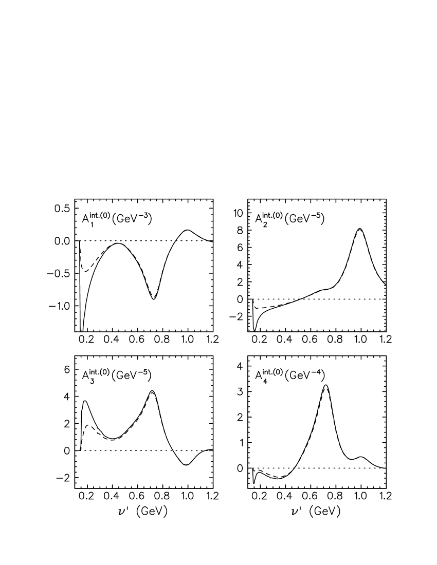
Figure 3: The integrands of eqs. (2) and (2) for the amplitudes $A_{i}^{(0)}$ obtained with $\nu=\nu_{\rm{thr}}$ (solid lines) and $\nu=0$ (dashed lines).

The integrands for the amplitudes $A_{i}^{(0)}$ are displayed in the following fig. 3 Since the isoscalar photon can not excite the $\Delta$ resonance, we now find a competition of contributions from the second and third resonance regions plus a large cusp effect for $A_{1}^{(0)}$. Altogether these integrands are considerably smaller than in the case of the $A_{i}^{(+)}$.

The presented integrands show a reasonable convergence for the higher energies. In fig. 4 we investigate the question of convergence further by decomposing the imaginary parts of the amplitudes into a partial wave series. The figure shows the dispersive part of the $\gamma p\to\pi^{0}p$ amplitudes as function of $\nu$ and at $t=t_{\rm{thr}}$. While both S and P waves in the imaginary part yield large contributions to $A_{1}$, the other three amplitudes are essentially determined by the P waves, with some higher partial wave contributions in the case of $A_{2}$ and $A_{3}$.

Since we want to extrapolate the amplitudes into the unphysical region at small $t$ values, we also study the dispersive parts of the isospin amplitudes as function of $\nu$ for a series of $t$ values in the range $M_{\pi}^{2}>t>-10M_{\pi}^{2}$. As shown in fig. 5, the $t$ dependence develops quite a regular pattern, with the cusp moving to larger $\nu$ values with increasing values of $t$. At the same time the physical threshold (see the line $\theta=180^{\circ}$ in fig. 1) moves to smaller values of $\nu$ down to the minimum at $\nu=\nu_{\rm{thr}}$, from whereon it increases again (see the line $\theta=0$ in fig. 1).

The comparison with the experiment Sch01 in fig. 6 shows that the dispersion integral by itself misses the threshold data for the amplitudes $A_{2}-A_{4}$. If we add the t-channel $\rho$ and $\omega$ poles according to MAID05, we obtain an almost perfect agreement for $A_{1}$, $A_{2}$ and $A_{4}$. The apparent discrepancy between theory and experiment for $A_{3}$ is an open question, which will be discussed later.

After these tests we feel safe to expand the amplitudes about the unphysical point at $\nu=0$ and $t=M_{\pi}^{2}$ where all the involved particles are on their mass shell. For this purpose we proceed as in our previous work Pas05 by casting the first amplitude in the form:

$$A_{1}^{\rm{disp}}(\nu,t) = A_{1}(\nu,t)-A_{1}^{\rm{pole}}(\nu,t)$$ (48)

$$= \frac{eg_{\pi N}}{2M_{N}^{2}}\,\left(\kappa+\Delta_{1}(\nu,t)\right)\,,$$

where $\kappa$ is the anomalous magnetic moment in the respective isospin or physical channel and $\Delta_{1}(\nu,t)$ the dimensionless “FFR discrepancy”. For convenience we also express the three other amplitudes by dimensionless functions $\Delta_{i}(\nu,t)$,

$$A_{2}^{\rm{disp}}(\nu,t) = \frac{eg_{\pi N}}{2M_{N}^{4}}\,\Delta_{2}(\nu,t)\,,$$

$$A_{3,4}^{\rm{disp}}(\nu,t) = \frac{eg_{\pi N}}{2M_{N}^{3}}\,\Delta_{3,4}(\nu,t)\,.$$ (49)

The functions $\Delta_{i}(\nu,t)$ are regular near the origin of the Mandelstam plane and can be expanded in a power series in $\nu$ and $t$ or $\nu_{B}$. As is evident from eq. (5), $\nu$ is ${\mathcal{O}}(M_{\pi})$ and $\nu_{B}$ is ${\mathcal{O}}(M_{\pi}^{2}/M_{N})$ in the region of interest. Therefore the crossing-even amplitudes $\Delta_{1,2,4}^{(+,0)}$ and $\Delta_{3}^{(-)}$ have the expansion

$$\Delta(\nu,t) = \delta_{00}+\delta_{20}\,\nu^{2}/M_{\pi}^{2}+\delta_{02}\,\nu_{B}/M_{\pi}+\delta_{40}\,\nu^{4}/M_{\pi}^{4}$$ (50)

$$+\delta_{22}\,\nu^{2}\nu_{B}/M_{\pi}^{3}+\delta_{04}\,\nu_{B}^{2}/M_{\pi}^{2}+\ldots\,,$$

with the lowest expansion parameters given by

$$\delta_{00} = \Delta(0,\,M^{2}_{\pi})\,,$$

$$\delta_{20} = \frac{M_{\pi}^{2}}{2}\frac{\partial^{2}}{\partial\,\nu^{2}}\,\Delta(\nu\,,M^{2}_{\pi})\big{|}_{\nu=0}\,,$$

$$\delta_{02} = 4M_{N}\,M_{\pi}\frac{\partial}{\partial\,t}\,\Delta(0,t)\big{|}_{t=M^{2}_{\pi}}\,.$$ (51)

In the case of the crossing-odd amplitudes $\Delta_{3}^{(+,0)}$ and $\Delta_{1,2,4}^{(-)}$ the corresponding expansion takes the form

$$\Delta(\nu,t)=\delta_{10}\,\nu/M_{\pi}+\delta_{30}\,\nu^{3}/M_{\pi}^{3}+\delta_{12}\,\nu\nu_{B}/M_{\pi}^{2}+\ldots\,,$$ (52)

with the lowest expansion parameter

$$\delta_{10}=M_{\pi}\frac{\partial}{\partial\nu}\,\Delta(\nu,M_{\pi}^{2})\big{|}_{\nu=0}\,.$$ (53)

In order to study the convergence of the multipole series involved in evaluating the dispersion integrals of eqs. (2) and (2) from the imaginary parts of the amplitudes, we compare the results obtained at $t=M^{2}_{\pi}$ with values obtained at different $t$. Table 1 shows our results for $\Delta_{1}^{(p\pi^{0})}(0,t)$ for $t=M_{\pi}^{2}$, 0, and $t_{\rm{thr}}$. The total value at $t=M^{2}_{\pi}$ corresponds to $\delta_{00}^{1}=-0.078$. The slow decrease with decreasing values of $t$ is due to the term $\delta_{02}\nu_{B}$.

t	$M_{\pi}^{2}$		$0$		$t_{\rm{thr}}$
$L=0$	$0$.	$571$	$0$.	$579$	$0$.	$586$
$L=1$	$1$.	$209$	$1$.	$150$	$1$.	$098$
$L=2$	$-0$.	$109$	$-0$.	$089$	$-0$.	$071$
$L=3$	$0$.	$044$	$0$.	$054$	$0$.	$062$
sum	$1$.	$715$	$1$.	$695$	$1$.	$676$

Table 1: Contributions of the dispersion integral to $\kappa_{p}+\Delta_{1}^{(p\pi^{0})}(0,t)$ at $t=M_{\pi}^{2}$, $0$, and $t_{\rm{thr}}$ for the $p\pi^{0}$ channel. The rows $L=0$ to $L=3$ indicate the contribution of the S, P, D, and F waves to the dispersion integral.

The following tables 2 and 3 show the $t$ dependence of the derivatives with regard to $\nu^{2}$ and $t$ at fixed $\nu=0$. The total values at $t=M_{\pi}^{2}$ yield the constants $\delta^{1}_{20}$ and $\delta^{1}_{02}$, respectively. The small changes with decreasing values of $t$ are due to the higher expansion coefficients $\delta^{1}_{22}$ and $\delta^{1}_{04}$. We note that the curvature in $\nu$ (table 2) is essentially determined by the S and P waves which add with a 1:2 ratio. However, the slope in $t$ (table 3) has considerable contributions from the higher partial waves. Although the P wave yields by far the largest contribution, the other partial waves conspire to reduce the total slope to less than 30% of the P-wave result.

t	$M_{\pi}^{2}$		$0$		$t_{\rm{thr}}$
$L=0$	$0$.	$11$	$0$.	$12$	$0$.	$12$
$L=1$	$0$.	$21$	$0$.	$21$	$0$.	$22$
$L=2$	$-0$.	$003$	$-0$.	$002$	$0$.	$000$
$L=3$	$-0$.	$000$	$0$.	$000$	$0$.	$000$
sum	$0$.	$32$	$0$.	$33$	$0$.	$34$

Table 2: Contributions of the dispersion integral to $\frac{M_{\pi}^{2}}{2}\frac{\partial^{2}}{\partial\,\nu^{2}}\,\Delta_{1}^{(p\pi^{0})}(\nu,t)$ for the $p\pi^{0}$ channel at fixed $\nu=0$. See table 1 for further notation.

t	$M_{\pi}^{2}$		$0$		$t_{\rm{thr}}$
$L=0$	$-0$.	$22$	$-0$.	$23$	$-0$.	$24$
$L=1$	$1$.	$62$	$1$.	$66$	$1$.	$71$
$L=2$	$-0$.	$54$	$-0$.	$57$	$-0$.	$59$
$L=3$	$-0$.	$29$	$-0$.	$26$	$-0$.	$24$
sum	$0$.	$57$	$0$.	$59$	$0$.	$63$

Table 3: Contributions of the dispersion integral to $4M_{N}\,M_{\pi}\frac{\partial}{\partial\,t}\,\Delta_{1}^{(p\pi^{0})}(0,t)$ for the $p\pi^{0}$ channel at fixed $\nu=0$. See table 1 for further notation.

	$\delta_{00}$		$\delta_{10}$		$\delta_{20}$		$\delta_{02}$
$A_{1}$	$-0$.	$08\ (+0.04)$	-		$0$.	$32$	$0$.	$57\ (+1.11)$
$A_{2}$	$-4$.	$54\ (-1.87)$	-		$-1$.	$26$	$3$.	$47\ (-1.55)$
$A_{3}$	-		$-2$.	$23$	-		-
$A_{4}$	$13$.	$02\ (+8.17)$	-		$2$.	$23$	$-2$.	$48\ (+6.98)$

Table 4: The leading expansion coefficients for the $p\pi^{0}$ amplitudes from the dispersion integral (see eqs. (48)-(53) for definitions) and the vector meson t-channel contributions (in brackets).

In table 4 we list the leading expansion coefficients of the 4 invariant amplitudes for the $p\pi^{0}$ channel. The additional contributions of the vector meson poles to the coefficients $\delta_{00}$ and $\delta_{02}$ are given in brackets. It is obvious that these $t$-channel effects play an important role in neutral pion photoproduction. The strong competition between $s$- and $t$-channel contributions to $\delta_{00}$ and $\delta_{02}$ reflects the previous discussion on subtracted DRs. According to eqs. (48)-(50) the subtraction functions $A_{i}^{I}(\nu=0,t)$ are determined by the respective expansion coefficients $\delta_{00}+\delta_{02}\nu_{B}/M_{\pi}+\cdots$, and on the other hand the DRs would sample information at $\nu=0$ from both $t$-channel reactions (for $t>0$) and $s$-channel reactions extrapolated into the unphysical region (for $t<0$).

The numbers in table 4 should be compared to an expansion of the loop plus counter terms in covariant BChPT. Such a calculation has been performed in Ref. Ber05 by evaluating the third-order loop corrections and supplementing them by a fourth-order polynomial. Since the fourth-order loop corrections are large, the resulting power series is only indicative of the expected LECs Ber05 . However, the coefficients compare favorably with the LECs obtained from the earlier HBChPT calculations Ber96 . Including for consistency an additional factor $e$ on the RHS, we obtain from eq. (2) of Ref. Ber05 the following coefficients from the fourth-order polynomial contribution: $\delta_{00}^{1}=0$, $\delta_{20}^{1}=0.53$, $\delta_{02}^{1}=3.40$, $\delta_{00}^{2}=-6.33$, $\delta_{10}^{3}=-2.58$, and $\delta_{00}^{4}=22.4$. These numbers are in qualitative agreement with our results in table 4. The differences are due to

1. the power series expansion of the loop corrections, which has to be added to the polynomial,

2. the effects of higher partial waves, particularly with regard to the t-dependence given by $\delta_{02}$, and

3. possible s-channel resonances above 2.2 GeV and t-channel exchange of heavier objects, not included in the dispersive approach.

As we have shown, the dispersion calculation including the vector meson poles is able to reproduce the experimental threshold data except for the crossing-odd amplitude $A_{3}$. In order to pin down the origin of this discrepancy, we have checked the integrands of the dispersion integrals by repeating our calculation with the SAID SAID analysis. Whereas the real parts of the MAID and SAID multipoles differ in some cases, particularly at the higher energies, the imaginary parts generally agree well for $W\lesssim 2.2$ GeV. As shown in fig. 6 the dispersive contributions of the two models turn out to be quite similar. Whereas the experimental threshold values for $A_{2}$ and $A_{4}$ can be described after adding the vector meson pole contributions, no such remedy exists for the crossing-odd amplitude $A_{3}$ for which both SAID and MAID are off by a factor of 2. We have also checked the high-energy contributions by varying the onset of the asymptotic tail in the range 1.8 GeV$\leqslant W\leqslant 2.5$ GeV and its shape from a simple $1/W$ dependence to various Regge prescriptions. In this way we can modify the threshold amplitudes $A_{1}^{thr}$, $A_{2}^{thr}$, and $A_{4}^{thr}$ by at most 10 % in the $\pi^{0}p$ channel. However, the asymptotic contribution to $A_{3}^{thr}$ reaches at most 1 % because of the better convergence for this crossing-odd amplitude.

We have also directly estimated the high-energy tail with the parameters given by the Regge models of the 1970’s Dev74 ; Bar74 , which were constructed to fit the data in the 5-20 GeV region. Since these models include the exchange of axial vector mesons and Regge cuts corresponding to many-particle exchange, they also contribute to the crossing-odd amplitude $A_{3}$. However, the predicted strength of the high-energy contribution to $A_{3}^{thr}$ turns out to be even smaller and of the order $10^{-3}$ only. On the phenomenological level, possible candidates for axial vector meson exchange ($J^{PC}=1^{++}$) are the $a_{1}\ (1260)$ with quantum numbers $I^{G}=1^{-}$ and the $f_{1}\ (1285)$ with $I^{G}=0^{+}$. The $a_{1}$ has the same isospin and $G$ parity as the pion, and therefore contributes only for charged pion production. The $f_{1}$, on the other hand, has positive $G$ parity and a branching ratio of about 5 % for the $\gamma\rho^{0}$ channel. It is therefore a good candidate for $\rho$ meson photoproduction and, together with the $a_{1}$, also for the Regge tail of the helicity-dependent inclusive cross sections as measured by the Gerasimov-Drell-Hearn experiment Bia99 . However, there appear to be no clear candidates to solve the $A_{3}$ puzzle by a t-channel pole term.

Let us finally discuss the multipole content of the relativistic amplitudes and the related error bars in the threshold region. As in our previous analysis we subtract the nucleon pole terms, which may vary within about 2 % depending on the value chosen for the pion-nucleon coupling constant $g_{\pi N}$. Since the pole term constitutes about 85 % of the total threshold amplitudes $A_{2}^{thr}$ and $A_{3}^{thr}$, the choice of $g_{\pi N}$ leads to an error of about 12 % in the remaining dispersive amplitudes. For $A_{1}^{thr}$ and $A_{4}^{thr}$, however, the pole contributions are small and therefore the model error of $g_{\pi N}$ can be neglected with regard to the dispersive amplitudes. In table 5 the threshold amplitudes are constructed from the experimental values of the S- and P-wave multipoles and the MAID05 value for the D waves. The error given in the table is obtained by adding the experimental errors for the threshold multipoles. We recall at this point that here and in the following all values refer to the dispersive contributions only.

As is evident from table 5, $A_{1}^{thr}$ is dominated by the S-wave, because the magnetic contributions cancel nearly completely. The large S-wave contribution originates from the FFR current Pas05 and rescattering corrections, which are of course included in BChPT by the chirally invariant pion-nucleon coupling and the pion loops leading to the pronounced cusp effect at the $n\pi^{+}$ threshold. These effects are nicely reproduced by the dispersion integral, and the small t-channel pole contribution is well within the experimental error bars. More precisely, the vector mesons produce large effects of about equal size for both magnetic multipoles, but the discussed cancellation between $M_{1+}$ and $M_{1-}$ leads to a reduction by a large factor.

Quite different physical information is sampled by $A_{2}^{thr}$. Due to the structure of the associated four-vector $M_{2}^{\mu}$, the spin $J=1/2$ multipoles $E_{0+}$ and $M_{1-}$ do not appear in this amplitude. It is dominated by $M_{1+}$ but also receives surprisingly large contribution from the D waves whose threshold values are not very well known. In HBChPT Ber96 about 90 % of this amplitude are obtained from counter terms.

In the case of $A_{3}^{thr}$ we again find a large cancellation of the magnetic multipole contributions, which is required because the $\rho$ and $\omega$ pole terms have to cancel exactly for symmetry reasons. However, the dispersive contributions of $M_{1+}$ and $M_{1-}$ are now large compared to $E_{0+}$, and this cancellation leads to a large error bar. The amplitude $A_{3}$ shows a weak cusp effect, in accordance with the result of HBChPT Ber96 .

Finally, the amplitude $A_{4}^{thr}$ is determined by the $\Delta(1232)$ multipole $M_{1+}$ and a remarkably strong Roper multipole $M_{1-}$. Since no cancellation appears among the dispersive contributions, the error bar of this amplitude is small. Similarly as in the case of $A_{2}^{thr}$, the amplitude $A_{4}^{thr}$ is almost totally determined by counter terms in both HBChPT Ber96 and covariant BChPT Ber05 .

	$E_{0+}$	$E_{1+}$	$M_{1+}$	$M_{1-}$	$D$	total
$A_{1}$	$4.75$	$0.08$	$2.02$	$-1.94$	$0.08$	$5.00\pm 0.25$
$A_{2}$	$0$	$-0.34$	$-29.44$	$0$	$5.13$	$-24.7\pm 5.9$
$A_{3}$	$2.36$	$-0.65$	$-18.67$	$14.34$	$-0.65$	$-3.3\pm 1.7$
$A_{4}$	$2.36$	$0.04$	$40.55$	$14.34$	$0.04$	$57.3\pm 1.9$

Table 5: The multipole decomposition of the dispersive part of the experimental threshold amplitudes, constructed from the data of Ref. Sch01 and the MAID05 value for the D-state contributions. The errors include statistical and systematic errors from the experiment and model errors due to uncertainties from the pion-nucleon coupling and from the D waves, all added in quadrature.

6 Summary and Outlook 

We have studied the photoproduction of pions by means of dispersion relations at $t=const$ for the relativistic amplitudes $A_{1}$ to $A_{4}$, using the imaginary parts of the amplitudes as input to evaluate the real parts. The calculations are performed with and compared to the most recent version MAID05, and it is our final goal to put this analysis on the basis of dispersion theory. Along these lines the present exploratory work on neutral pion photoproduction has the aim to (I) test the numerical procedure and the data basis by trying to reproduce the precision data near threshold and (II) predict the low-energy constants of baryon chiral perturbation theory (BChPT) by global properties of the excitation spectrum.

After subtraction of the nucleon and pion pole terms, the remaining “dispersive” amplitudes are regular functions of the Mandelstam variables in the subthreshold region. In particular they may be expanded in a power series in the two independent variables $\nu$ and $t$ about the point $\nu=0$, $t=M_{\pi}^{2}$. This series converges in a circle with a radius determined by the threshold of pion production. The singularity at threshold is, of course, well described by the loop corrections of BChPT, which also can be expanded in a power series below threshold. The difference of the expansions of the full amplitude and the loop contribution is described by the low-energy constants necessary to apply BChPT to the data analysis.

We find that the threshold amplitude $A_{1}^{thr}$ is well described by the dispersion integral within the experimental error. As in our previous work we also obtain a good agreement with the FFR sum rule that connects the amplitude $A_{1}$ to the anomalous magnetic moment of the nucleon. In the case of $A_{2}^{thr}$ and $A_{4}^{thr}$, however, we have to include additional contributions of t-channel vector meson exchange. The importance of such effects for neutral pion photoproduction has been noted long ago. As was to be expected, our calculations also show that these fixed poles at $t=m_{V}^{2}$ can not be obtained from the dispersion integrals. Moreover, though these mesons play an important role for the unitarization process at the higher energies, their global effect on the dispersion integrals for the threshold amplitudes is surprisingly small. If we add the vector meson pole terms to the dispersion integrals, we obtain a considerable improvement also for $A_{2}^{thr}$ and $A_{4}^{thr}$, and a perfect fit would require only a modest change of the coupling constants with respect to the MAID values.

However, the predicted value for $A_{3}^{thr}$ is at variance with the data by more than 2 standard deviations. This is a serious problem for the crossing-odd amplitude $A_{3}$, because a t-channel pole contribution requires the exchange of an axial vector meson. Unfortunately, the known axial vector mesons have either the wrong isospin or the wrong G parity for neutral pion photoproduction.

In view of the apparent discrepancy for $A_{3}^{thr}$ we have carefully checked all the ingredients of our calculation. We have repeated the integrations using the absorptive amplitudes given by SAID SAID . In spite of occasional differences between the MAID and SAID multipole analyses, particularly at energies $W\gtrsim 2$ GeV, both models predict quite similar amplitudes up to the $\Delta(1232)$ resonance. We have further studied the influence of the high-energy region by varying the upper limit of integration in the range of 1.8 GeV$\leqslant W\leqslant 2.5$ GeV and by fitting the high-energy tail with various shapes from a simple $1/W$ behavior to several Regge forms. In this way the threshold amplitudes change by about 5 % for $A_{1}^{thr}$ and a few per cent for $A_{2}^{thr}$ and $A_{4}^{thr}$, whereas the possible error for $A_{3}^{thr}$ is less than 1 %. If we directly apply various Regge models, including phenomenological Regge poles and cuts, the high-energy contribution turns out to be even smaller, particularly in the case of $A_{3}^{thr}$. Even independent of any model assumption, the crossing-odd amplitude $A_{3}$ has the best convergence property of all the amplitudes, and therefore an extremely strong asymptotic contribution would be necessary to change $A_{3}^{thr}$ by a factor of 2.

As we have shown, the experimental error for $A_{3}^{thr}$ is very large due to a near total cancellation between the leading magnetic multipoles. For this reason the D state contribution may give rise to some concern. Its contribution has been estimated to account for about 20 % of $A_{3}^{thr}$, which assumption is based on a reasonable extrapolation to the threshold region. However, local fits in certain energy bins often yield large fluctuations of the D-state background. Therefore a large model error for this background can not be excluded and may be partially responsible for the $A_{3}$ problem.

With all these caveats in mind we have evaluated the dispersive and vector meson contributions of the relativistic amplitudes and expanded the result in a power series in $\nu$ and $t$ as discussed in detail in the previous section. The results nicely compare with the low-energy constants derived from a fit of covariant BChPT to the threshold data. Except for the $A_{3}$ problem, the differences between the two approaches are due to additional loop terms. In view of the unexpectedly large loop corrections at $4^{\rm{th}}$ order HBChPT, an extension of the existing $3^{\rm{rd}}$ order covariant BChPT to the next order will be of great general interest.

On the side of the dispersive approach, the simple addition of the vector meson pole terms to the dispersive amplitude is of course only justified near threshold where the scattering phases are small. In general it will be necessary to unitarize the full amplitude comprising the nucleon, pion, and vector meson pole terms as well as the complex contribution of the continuum. This will require an iterative procedure including modifications of the model parameters encoded in the helicity amplitudes of the resonances. A further challenge is to describe the gradual transition from vector meson poles near threshold to Regge propagators at large energies, without introducing spurious singularities and respecting the crossing symmetry of the invariant amplitudes.

In view of the large D-wave background and the delicate cancellation of various multipoles in $A_{3}^{thr}$, dedicated experiments to measure the D-wave contribution in the region between threshold and the $\Delta(1232)$ resonance would be extremely helpful. Whereas the difference of recoil and target polarization in forward direction is directly proportional to the amplitude $A_{3}$ in the high-energy limit, this observable does not appear to be very sensitive to $A_{3}$ in the threshold region. We are presently studying several double-polarization observables with regard to an enhanced sensitivity for $A_{3}$ and the D-wave background.

Figure 1: The Mandelstam plane for the isospin $I=+$ as function of $\nu$ and $t$. Solid lines: the boundaries of the physical region between forward ($\theta=0$) and backward ($\theta=180^{o}$) scattering. Dashed lines: the boundaries of the st and su spectral regions. The dashed-dotted line is obtained by reflecting the st boundary at the dotted line $\theta=90^{o}$. The other dotted lines indicate the asymptotic boundaries of the spectral regions. The left half-plane, which is not shown here, is determined by the crossing symmetry, $\nu\rightarrow-\nu$ or $s\leftrightarrow u$. See text for further explanation.

Figure 2: The integrands of eqs. (2) and (2) for the amplitudes $A_{i}^{(+)}$ obtained with $\nu=\nu_{\rm{thr}}$ (solid lines) and $\nu=0$ (dashed lines).

Figure 4: The real parts of the amplitudes $A_{i}^{(p\pi^{0})}$ for the reaction $\gamma p\to\pi^{0}p$ as function of $\nu$ and at $t=t_{\rm{thr}}$. Solid lines: Dispersive contributions according to eqs. (2) and (2) as obtained with the imaginary amplitudes from MAID05 containing partial waves up to $L_{\rm{max}}=3$. Short-dashed lines: S-wave contributions, dotted lines: P-wave contributions, long-dashed lines: Sum of D- and F-wave contributions. The dashed-dotted lines starting at pion threshold show the real parts taken directly from MAID05.

Figure 5: The real parts of the amplitudes $A_{i}^{(+)}$ as function of $\nu$. The dispersive contributions according to eqs. (2) and (2) as evaluated with the imaginary amplitudes from MAID05 for the following values of $t$: $M_{\pi}^{2}$ (solid lines), $t_{\rm{thr}}$ (dashed lines), $-4M_{\pi}^{2}$ (dashed-dotted lines), and $-10M_{\pi}^{2}$ (dotted lines).

Figure 6: The real parts of the amplitudes $A_{i}^{(p\pi^{0})}$ for the reaction $\gamma p\to\pi^{0}p$ as function of $\nu$ and at $t=t_{thr}$. Solid lines: dispersive contributions according to eqs. (2) and (2) as evaluated with the imaginary amplitudes from MAID05 containing partial waves up to $L_{\rm{max}}=3$. Dashed lines: same results calculated with SAID. The dashed-dotted lines are obtained by adding the vector-meson contributions of eq. (45) to the MAID result. The data points near threshold are derived from the experimental values of Ref. Sch01 for the S and P waves plus the MAID correction for the D waves.

References

- (1) B. Pasquini, D. Drechsel, and L. Tiator, Eur. Phys. J. A 23 (2005) 279.
- (2) S. Fubini, G. Furlan, and C. Rossetti, Nuovo Cim. 40 (1965) 1171.
- (3) D. Drechsel, O. Hanstein, S.S. Kamalov, and L. Tiator, Nucl. Phys. A 645 (1999) 145; http://www.kph.uni-mainz.de/MAID/.
- (4) R. Beck et al., Phys. Rev. Lett. 65 (1990) 1841.
- (5) V. Bernard, N. Kaiser, J. Gasser, and U.-G. Meißner, Phys. Lett. B 268 (1991) 291; V. Bernard, N. Kaiser, and U.-G. Meißner, Nucl. Phys. B 383 (1992) 442.
- (6) T. Becher and H. Leutwyler, Eur. Phys. C 9 (1999) 643; B. Kubis and U.-G. Meißner, Nucl. Phys. A 679 (2001) 698; T. Fuchs, J. Gegelia, G. Japaridze, and S. Scherer, Phys. Rev. D 68 (2003) 056005.
- (7) V. Bernard, B. Kubis, and U.-G. Meißner, Eur. Phys. J. A 25 (2005) 419.
- (8) G.F. Chew et al., Phys. Rev. 106 (1957) 1345.
- (9) O. Hanstein, D. Drechsel, and L. Tiator, Nucl. Phys. A 632 (1998) 561.
- (10) J.D. Bjorken and S.D. Drell, Relativistic Quantum Fields, McGraw-Hill, New York (1965).
- (11) S. Mandelstam, Phys. Rev. 112 (1958) 1344; 115 (1959) 1741; 115 (1959) 1752.
- (12) See, e.g., S.C. Frautschi and J.D. Walecka, Phys. Rev. 120 (1960) 1486; W.R. Frazer and J.R. Fulco, Phys. Rev. 119 (1960) 1420.
- (13) J.S. Ball, Phys. Rev. 124 (1961) 2014.
- (14) E.T. Whittaker and G.N. Watson, Modern Analysis, p. 322, Cambridge University Press (1958).
- (15) R. Oehme and J.G. Taylor, Phys. Rev. 113 (1959) 371.
- (16) G. v. Gehlen, Nucl. Phys. B 9 (1969) 17.
- (17) D. Drechsel, B. Pasquini and M. Vanderhaeghen, Phys. Rep. 378 (2003) 99.
- (18) M. Guidal, J.-M. Laget, and M. Vanderhaeghen, Nucl. Phys. A 627 (1997) 645 and Phys. Lett. B 400 (1997) 6.
- (19) I.G. Aznauryan, Phys. Rev. C 67 (2003) 015209.
- (20) R.C.E. Devenish, D.H. Lyth, and W.A. Rankin, Phys. Lett. 52B (1974) 227.
- (21) I.S. Barker, A. Donnachie, and J.K. Storrow, Nucl. Phys. B 79 (1974) 431.
- (22) S. S. Kamalov, S. N. Yang, D. Drechsel, O. Hanstein and L. Tiator, Phys. Rev. C 64 (2001) 032201.
- (23) S. Eidelman et al., Phys. Lett. B 592 (2004) 1.
- (24) L. Tiator, D. Drechsel, S.S. Kamalov, and S.N. Yang, Eur. Phys. J. A 17 (2003) 357.
- (25) L. Tiator, D. Drechsel, S.S. Kamalov, M.M. Giannini, E. Santopinto, and A. Vassallo, Eur. Phys. J. A 19 (2004) 55.
- (26) S. S. Kamalov, L. Tiator, D. Drechsel, R. A. Arndt, C. Bennhold, I. I. Strakovsky and R. L. Workman, Phys. Rev. C 66 (2002) 065206.
- (27) A. Schmidt et al., Phys. Rev. Lett. 87 (2001) 232501.
- (28) V. Bernard, N. Kaiser, and U.-G. Meißner, Z. Phys. C 70 (1996) 483; V. Bernard, N. Kaiser, and U.-G. Meißner, Phys. Lett. B 378 (1996) 337; V. Bernard, N. Kaiser, and U.-G. Meißner, Eur. Phys. J. A 11 (2001) 209.
- (29) R.A. Arndt, W.J. Briscoe, I.I.Strakovsky, and R.L. Workman, Phys. Rev. C 66 (2002) 055213; http://gwdac.phys.gwu.edu/.
- (30) N. Bianchi and E. Thomas, Phys. Lett. B 450 (1999) 439.