Few body impulse and fixed scatterer approximations for high energy scattering

Abstract

The elastic scattering differential cross section is calculated for proton scattering from ⁶He at 717 MeV, using single scattering terms of the multiple scattering expansion of the total transition amplitude (MST). We analyse the effects of different scattering frameworks, specifically the Factorized Impulse Approximation (FIA) and the Fixed Scatterer (adiabatic) Approximation (FSA) and the uncertainties associated with the use different structure models.

I Introduction

The understanding of nuclei can only be fully achieved by studying the way they interact with other nuclei. This is particularly true for halo nuclei, due to their short lifetime and simplified energy spectrum. We consider here the scattering of a structureless projectile by a target assumed to be composed of structureless subsystems (as is approximately the case for halo nuclei).

It is the aim of a microscopic reaction theory to construct the total scattering amplitude in terms of well defined dynamical and structural quantities. For the scattering of a nucleon by a target with ${\cal N}$ particles, one has to solve a $n={\cal N}+1$ many body scattering problem. For ${\cal N}=2$ clusters of equal mass this has been done solving the Faddeev equations Joa87 and generalized for ${\cal N}=3$ Alt70 ; Fon84 . This many body scattering framework is however very complicated, and does not handle clusters of different mass, and so alternative methods have been developed as for example the Continuum Discretized Coupled Channels (CDCC). In this approach a system of coupled equations needs to be solved with effective projectile-subsystem interactions. This method has been successfully applied for more than two decades to the scattering of (${\cal N}=2$)-body targets for a wide range of projectile masses and bombarding energies. The case of the scattering from a (${\cal N}=3$)-body system is considerably more demanding, although some work is already in progress Mat04 . Alternatively in the high energy regime one can use a multiple scattering expansion of the total transition amplitude, MST Gol64 ; Wat57 ; Joa87 ; Cres99 ; Cres02 ; CresRNB .

When describing the scattering of stable from halo nuclei, it is crucial to model the halo many-body character of ${\cal N}$ composite particles Cres99 ; Cres02 ; CresRNB . In particular, a three or four-body problem has to be solved when studying the scattering of a projectile by a target which is a bound state of two or three subsystems, as is the case for ¹¹Be and ⁶He respectively.

This problem can be conveniently addressed by the MST approach. In this formalism, the projectile-target transition amplitude is expanded in terms of off-shell transition amplitudes for projectile-subsystem scattering. Due to the complexity of the many-body operator, suitable approximations need to be made in order to express in a convenient way the overall scattering amplitude in terms of the scattering by each target subsystem. Under further suitable approximations each term can be written in terms of a product of a form factor and the transition amplitude for the scattering for that subsystem. The MST method provides a clear and transparent interpretation of the scattering of a composite system in terms of the free scattering of its constituents and is numerically advantageous. This scattering framework is particularly useful at high energies and for loosely bound nuclei where the expansion is expected to converge quickly.

In this paper, we use this framework to calculate the elastic scattering differential cross section for proton scattering on ⁶He at 717 MeV where new data has been obtained at higher transferred momentum than previously. These new momentum transfers, however, still essentially probe only that part of the few-body dynamics of the halo cluster which is constrained by the rms radius. Therefore the few-body treatment of the halo is appropriate in this energy and angular range, and we will see that calculated differential cross sections for various structure models largely reflects properties closely connected to rms radii. It is the aim of the present paper to clarify and test the approximations involved in the applying the MST multiple scattering expansion to find the predicted cross sections for proton-halo elastic scattering at these momentum transfers. Specifically, we examine (i) the impulse approximation, (ii) the factorization approximations and (iii) the single scattering approximation.

II Multiple scattering expansion of the total transition amplitude

We consider the scattering of a projectile (system 1) from a few-body target consisting of ${\cal N}$ sub-systems weakly bound to each other. We shall frequently refer to the composite system as the target although in practice an actual experiment may be carried out with the composite system as a projectile. The subsystems ${\cal I},{\cal J},\ldots$ are assumed to be stable and can be either composite nuclei or nucleons. The total transition amplitude for the scattering is

$$T = V+VGT$$ (1)

$$= \sum_{{\cal I}=2}^{n}v_{\cal I}+\sum_{{\cal I}=2}^{n}v_{\cal I}GT~{}~{},$$

with $n={\cal N}+1$, $v_{\cal I}$ the interaction between the projectile and the ${\cal I}$ target subsystem, and $G$ is the propagator

$$G=\left(E^{+}-K-\sum V_{{\cal I}{\cal J}}\right)^{-1}.$$ (2)

Here, $E$ is the total energy and is related to the total incident kinetic energy $E_{1}=\frac{\hbar^{2}k_{1}^{2}}{2\mu_{NA}}$ by $E=E_{1}+\epsilon_{0}$ where $\epsilon_{0}$ is the target ground state energy. At this stage we use non-relativistic kinematics. The inclusion of relativistic kinematics will be discussed later. The operator $K$ corresponds to the total kinetic energy of the projectile and ${\cal N}$ target sub-systems in the projectile-target center of mass frame. In Eq. (2) $V_{{\cal I}{\cal J}}$ is the interaction between subsystems ${\cal I}$ and ${\cal J}$. Equivalently, we may write the propagator in terms of the kinetic energy operator for the projectile $K_{1}$ in the center of mass of the interacting projectile-target (P-T) system, and the target nucleus Hamiltonian, $H_{0}$

$$G=\left(E^{+}-K_{1}-H_{0}\right)^{-1}.$$ (3)

The total transition amplitude, Eq.(1), can be rewritten as

$$T=\sum_{\cal I}\tau_{\cal I}+\sum_{\cal I}\tau_{\cal I}G\sum_{{\cal J}\neq{\cal I}}\tau_{\cal J}+\cdots~{}~{}.$$ (4)

where the projectile-${\cal I}$ subsystem transition amplitude $\tau_{\cal I}$ is given by

$$\tau_{\cal I}=v_{\cal I}+v_{\cal I}G\tau_{\cal I}~{}~{}.$$ (5)

We note that the propagator in $\tau_{\cal I}$ contains the target Hamiltonian and thus it is still at this stage a many-body operator. In the limit when the target nucleus subsystems are weakly bound to each other, the multiple scattering expansion to the P-T transition amplitude is expected to converge rapidly Wat57 ; Gol64 and the MST expansion Eq. (4) can be used.

We apply next this formalism to proton scattering from a target of two and three bound structureless subsystems.

III The Single scattering 3-body problem

We first consider the scattering of a projectile of mass $m_{1}$ from a target (such as ¹¹Be) assumed to be well described by a two body model with two subsystems (of valence particle and a core) labeled here as 2 and 3 of masses $m_{2}$ and $m_{3}$ respectively. Let $\vec{k}_{1},\vec{k}_{2},\vec{k}_{3}$, ($\vec{k}^{\prime}_{1},\vec{k}^{\prime}_{2},\vec{k}^{\prime}_{3}$) be the initial (final) momenta of the projectile and the two cluster subsystems.

Neglecting core excitation, the target wave function is

$$\Phi(\vec{r},{\xi}_{3})=\left[\phi_{23}(\vec{r})\otimes\varphi_{3}({\xi}_{3})\right]~{}~{},$$ (6)

where $\varphi_{3}({\xi}_{3})$ is the core internal wave function and $\phi_{23}$ is the wave function describing the relative motion of the (2,3) pair.

The elastic transition amplitude to first order in the projectile-subsystem transition amplitudes is

$$T = \langle\vec{k}^{\prime}_{1}\Phi|\tau_{2}|\vec{k}_{1}\Phi\rangle+\langle\vec{k}^{\prime}_{1}\Phi|\tau_{3}|\vec{k}_{1}\Phi\rangle+\cdots$$ (7)

There are two approaches in handling the dynamics of the few-body system: The impulse (I) and the Fixed Scatterer (or frozen halo, or adiabatic) (FS) approach. They are related in high energy regime for special cases of the scattering amplitudes.

III.1 The factorized impulse approximation [FIA]

Within the impulse approximation, the interaction between the clusters $V_{{\cal I}{\cal J}}$ is assumed to have a negligible dynamical effect on the scattering of the projectile from the individual target subsystems and therefore can be neglected. The operator projectile-${\cal I}$ target subsystem transition amplitude $\tau_{\cal I}$ is then replaced by

$$\hat{t}_{\cal I}=v_{\cal I}+v_{\cal I}\hat{G}_{0}\hat{t}_{\cal I}$$ (8)

where $\hat{G}_{0}$ contains only the kinetic energy operator $K$

$$\hat{G}_{0}=\left(E^{+}-K\right)^{-1}~{}~{}.$$ (9)

The transition amplitude $\hat{t}_{\cal I}$ is still a many body operator, because the kinetic energy operator has contributions from the projectile and all ${\cal N}$ target subsystems. The interaction between the target subsystems leads to terms in 3rd order of the $\hat{t}_{\cal I}$ transition amplitude. As we shall see, this projectile-${\cal I}$ subsystem amplitude can be reduced, after suitable approximations, to a free two-body amplitude evaluated at the appropriate energy. Accepting the validity of replacing $\tau_{\cal I}$ by $\hat{t}_{\cal I}$ in Eq. (4) we obtain the multiple scattering expansion

$$T^{\rm IA}=\sum_{\cal I}\hat{t}_{\cal I}+\sum_{\cal I}\hat{t}_{\cal I}\hat{G}_{0}\sum_{{\cal J}\neq{\cal I}}\hat{t}_{\cal J}+\cdots$$ (10)

In the single scattering approximation (SA) only the first term is taken into account.

Let us consider the scattering from subsystem ${\cal I}=2$. Because from the dynamical point of view we want to reduce the problem to the projectile scattering from each subsystem, we take as relevant coordinates the relative momentum between projectile and subsystem ${\cal I}$=2, $\vec{q}_{1,2}$, and the relative momentum between the target subsystems, $\vec{q}_{2,3}$, defined here as

$$\vec{q}_{1,2}=\frac{m_{2}\vec{k}_{1}-m_{1}\vec{k}_{2}}{M_{12}}~{}~{},~{}~{}\vec{q}_{2,3}=\frac{m_{3}\vec{k}_{2}-m_{2}\vec{k}_{3}}{M_{23}}$$ (11)

where $M_{12}=m_{1}+m_{2},M_{23}=m_{2}+m_{3}$. In the three-particle c.m. frame, $\vec{\cal P}_{t}=\sum_{i=1}^{3}\vec{k}_{i}=0$ ($\vec{\cal P^{\prime}}_{t}=\sum_{i=1}^{3}\vec{k}\,^{\prime}_{i}=0$), and the propagator $\hat{G}_{0}$ is

$$\hat{G}_{0} = \left[E^{+}-\frac{\hbar^{2}}{2\mu_{12}}q^{2}_{12}-\frac{\hbar^{2}}{2\mu_{12,3}}k^{2}_{3}\right]^{-1}$$

$$= \left[E^{+}-\frac{\hbar^{2}}{2\mu_{12}}q^{2}_{12}-\frac{\hbar^{2}}{2\mu_{12,3}}\left(\vec{q}_{23}+\frac{m_{3}}{M_{23}}\vec{k}_{1}\right)^{2}\right]^{-1}$$

with $\mu_{12}=m_{1}m_{2}/M_{12}$ and $\mu_{12,3}=m_{3}M_{12}/M_{123}$, $M_{123}=m_{1}+m_{2}+m_{3}$. The total energy, neglecting binding effects, is

$$E=\frac{\hbar^{2}}{2\mu_{1,23}}k_{1}^{2}+\frac{\hbar^{2}}{2\mu_{23}}Q_{23}^{2}~{}~{},$$ (13)

with $\mu_{1,23}=m_{1}M_{23}/M_{123}$, and $\vec{Q}_{23}$ an average relative momentum between the target subsystems, to be specified below. The single scattering matrix elements are

$$\langle\vec{k}^{\prime}_{1}\phi_{23}|\hat{t}_{2}|\vec{k}_{1}\phi_{23}\rangle=\int d\vec{q}_{23}\phi^{*}_{23}\left(\vec{q}_{23}-\frac{m_{3}}{M_{{2}{3}}}\vec{\Delta}\right)$$

$$~{}~{}~{}~{}~{}~{}~{}\times\langle\vec{q}\,^{\prime}_{1,{2}}|\hat{t}_{2}(\hat{\omega}_{1{2}})|\vec{q}_{1,2}\rangle\phi_{23}\left(\vec{q}_{23}\right)~{}~{}.$$ (14)

Here, $\vec{\Delta}$ is the projectile momentum transfer

$$\vec{\Delta}=\vec{k}^{\prime}_{1}-\vec{k}_{1}~{}~{}.$$ (15)

The initial and final relative momenta between the projectile and the subsystem ${\cal I}=2$, $\vec{q}_{1,{2}}$ and $\vec{q}\,^{\prime}_{1,{2}}$ are respectively

$$\vec{q}_{1,{2}} = \frac{\mu_{12}}{\mu_{1,23}}\vec{k}_{1}-\frac{\mu_{1{2}}}{m_{2}}\vec{q}_{{2},{3}}=\beta_{12}\vec{k}_{1}-\alpha_{12}\vec{q}_{{2},{3}}~{}~{},$$

$$\vec{q}\,^{\prime}_{1,{2}} = \frac{\mu_{12}}{\mu_{1,23}}\vec{k}\,^{\prime}_{1}-\frac{\mu_{1{2}}}{m_{2}}\vec{q}\,^{\prime}_{{2},{3}}=\beta_{12}\vec{k}\,^{\prime}_{1}-\alpha_{12}\vec{q}\,^{\prime}_{{2},{3}}$$ (16)

$$= \frac{\mu_{12}}{\mu_{1,23}}\vec{k}\,^{\prime}_{1}-\frac{\mu_{1{2}}}{m_{2}}\vec{q}_{{2},{3}}+\frac{\mu_{1{2}}}{m_{2}}\frac{m_{3}}{M_{23}}\vec{\Delta}$$

$$= \beta_{12}\vec{k}\,^{\prime}_{1}-\alpha_{12}\vec{q}_{{2},{3}}+\alpha_{12}\gamma_{12}\vec{\Delta}~{}~{},$$

with $\beta_{12}=\mu_{12}/\mu_{1,23}$, $\alpha_{12}=\mu_{12}/m_{2}$, and $\gamma_{12}=\mu_{23}/m_{2}$. We shall use these whenever a simplified notation is required. These new parameters satisfy $\beta_{12}+\alpha_{12}\gamma_{12}=1$, from which it follows, together with Eq. (16), that the condition $\vec{q}\,^{\prime}_{1,2}-\vec{q}_{1,2}=\vec{\Delta}$ necessarily holds. The energy parameter $\hat{\omega}_{1{2}}$ is

$$\hat{\omega}_{1{2}}=E-\frac{\hbar^{2}}{\mu_{12,3}}\left(\vec{q}_{23}+\frac{m_{3}}{M_{23}}\vec{k}_{1}\right)^{2}~{}~{}.$$ (17)

The single-scattering matrix elements of Eq. (14) involve a full folding integral of a product of a transition amplitude and a target form factor. This integral may be quite involved. As we shall see below, in the high energy regime, the relative momentum of the interacting pair $\vec{q}_{23}$ can be approximated by a suitable value $\vec{\cal Q}_{23}$. Once replaced in Eqs. (16-17) one obtains a factorized impulse approximation (FIA) expression,

$$T^{\rm FIA}(E)=\langle\vec{\cal Q}\,^{\prime}_{12}|\hat{t}_{2}(\omega_{12})|\vec{\cal Q}_{12}\rangle\rho_{23}\left(\frac{m_{3}}{M_{23}}\vec{\Delta}\right)$$

$$~{}~{}~{}+\langle\vec{\cal Q}\,^{\prime}_{13}\phi_{3}|\hat{t}_{3}(\omega_{13})|\phi_{3}\vec{\cal Q}_{13}\rangle\rho_{23}\left(\frac{m_{2}}{M_{23}}\vec{\Delta}\right)~{}~{},$$ (18)

where $\vec{\cal Q}_{1{\cal I}}$ is approximate relative momentum projectile-subsystem ${\cal I}$, $\omega_{1{\cal I}}$ the energy parameter and $\rho_{23}$ the target form factor

$$\rho_{23}\left(\vec{\Delta}_{1}\right)=\int d\vec{q}_{23}\phi^{*}_{23}\left(\vec{q}_{23}-\vec{\Delta}_{1}\right)\phi_{23}\left(\vec{q}_{23}\right)$$ (19)

In the limit of a heavy subsystem $m_{3}\gg m_{2}$, we obtain the expected limit of $\rho_{23}\left(\frac{m_{2}}{M_{23}}\vec{\Delta}\right)=1$. Equivalently, we can write the scattering amplitudes in terms of the transferred momentum $\vec{\kappa}_{12}=\vec{\cal Q}\,^{\prime}_{12}-\vec{\cal Q}_{12}$ and total momentum ${\vec{\cal K}}_{12}=[\vec{\cal Q}\,^{\prime}_{12}+\vec{\cal Q}_{12}]/2$:

$$T^{\rm FIA}(E)=\hat{t}_{2}(\omega_{12},\vec{\kappa}_{12},\vec{\cal K}_{12})\rho_{23}\left(\frac{m_{3}}{M_{23}}\vec{\Delta}\right)$$

$$~{}~{}~{}+\hat{t}_{3}(\omega_{13},\vec{\kappa}_{13},\vec{\cal K}_{13})\rho_{23}\left(\frac{m_{2}}{M_{23}}\vec{\Delta}\right)~{}~{}.$$ (20)

The scattering amplitudes are on-shell if $|{\vec{\cal Q}}_{1{\cal I}}|$ = $|\vec{\cal Q}\,^{\prime}_{1{\cal I}}|$ = $\sqrt{2\mu_{1,{\cal I}}\omega_{1{\cal I}}}/\hbar$. In this case the scattering amplitudes are local. As we shall show below, although $\vec{q}\,^{\prime}_{1,2}-\vec{q}_{1,2}=\vec{\Delta}$, the approximate FIA may not satisfy $\vec{\kappa}_{12}=\vec{\Delta}$. The scattering amplitudes are related to the transition amplitude according to Joa87

$$|F(E)|^{2}=\frac{(2\pi^{2})^{4}}{\hbar v_{1}}k_{1}^{2}\frac{dk_{1}}{dE}|T(E)|^{2}$$ (21)

for projectile target scattering, and

$$|f_{\cal I}(\omega_{1{\cal I}})|^{2}=\frac{(2\pi^{2})^{4}}{\hbar v_{1}}k_{1}^{2}\frac{dk_{1}}{d\omega_{1{\cal I}}}|t_{\cal I}(\omega_{1{\cal I}})|^{2}$$ (22)

for projectile subsystem ${\cal I}$ scattering. The elastic differential angular distribution is then evaluated from the total scattering amplitude on-shell

$$F^{\rm FIA}(E)={\cal N}_{12}^{1/2}\hat{f}_{2}(\omega_{12},\vec{\kappa}_{12})\rho_{23}\left(\frac{m_{3}}{M_{23}}\vec{\Delta}\right)$$

$$~{}~{}~{}+{\cal N}_{13}^{1/2}\hat{f}_{3}(\omega_{13},\vec{\kappa}_{13})\rho_{23}\left(\frac{m_{2}}{M_{23}}\vec{\Delta}\right),$$ (23)

where the normalization factors are

$${\cal N}_{1{\cal I}}=\left[\frac{1}{d\omega_{1{\cal I}}/dE}\right]^{2}~{}~{}.$$ (24)

We now discuss several factorized impulse approximations that can be found in the literature. All these approximations use Eq. (14) as starting point. The differences between the models arise from the approximations performed to obtain a factorized expression of the form (18).

III.1.1 The 3b on-shell FIA [Kujawski and Lambert]

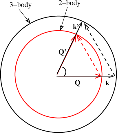
Figure 1: (Color online) Kinematics for the 3-body scattering in the impulse approximation of Kujawski and Lambert (KL). The dashed lines represent the momentum transfer for the case of the 3-body system (dashed dark line) and the 2-body system (dashed light line). The vectors $\vec{k}(\vec{k}\,^{\prime})$ represent the initial (final) projectile momenta, and $\vec{Q}(\vec{Q}\,^{\prime})$ the initial (final) projectile-subsystem ${\cal I}$ relative momenta.

In the factorized on-shell approximation, discussed in the work of Kujawski and Lambert (KL) Kuj73 , the incident and outgoing relative momenta of the subsystems $q_{23}(q^{\prime}_{23})$ are neglected by comparison with the projectile momentum. That is, inserting

$$|\vec{Q}_{23}|=0$$ (25)

into Eq. (16-17), one obtains for the relative momenta between the projectile and subsystem ${\cal I}=2$

$$\vec{\cal Q}_{12}=\frac{\mu_{12}}{\mu_{1,23}}\vec{k}_{1}~{}~{},~{}~{}\vec{\cal Q}\,^{\prime}_{12}=\frac{\mu_{12}}{\mu_{1,23}}\vec{k}\,^{\prime}_{1}~{}~{},$$ (26)

and for the energy parameter

$$\omega_{12} = \frac{\hbar^{2}}{2\mu_{12}}|\vec{\cal Q}_{12}|^{2}=\frac{\mu_{12}}{\mu_{1,23}}E~{}~{}.$$ (27)

Similar expressions are obtained for the scattering from subsystem ${\cal I}=3$

$$\vec{\cal Q}_{13}=\frac{\mu_{13}}{\mu_{1,23}}\vec{k}_{1}~{}~{},~{}~{}\vec{\cal Q}\,^{\prime}_{13}=\frac{\mu_{12}}{\mu_{1,23}}\vec{k}\,^{\prime}_{1}~{}~{},$$ (28)

and for the energy parameter

$$\omega_{13}=\frac{\mu_{1{3}}}{\mu_{1,23}}E~{}~{}.$$ (29)

The kinematics for the KL approximation is represented schematically in Fig. 1. Clearly, in this approach the relative projectile-subsystem ${\cal I}$ momentum is a fraction of the total transfered momentum $\vec{\Delta}$

$$\vec{\kappa}_{1{\cal I}}=\frac{\mu_{1{\cal I}}}{\mu_{1,23}}\vec{\Delta}~{}~{}.$$ (30)

The single scattering terms are then

$$T=\langle\frac{\mu_{12}}{\mu_{1,23}}\vec{k}\,^{\prime}_{1}|\hat{t}_{2}(\omega_{12})|\frac{\mu_{12}}{\mu_{1,23}}\vec{k}_{1}\rangle\rho_{23}\left(\frac{m_{3}}{M_{23}}\vec{\Delta}\right)$$

$$~{}~{}~{}+\langle\frac{\mu_{13}}{\mu_{1,23}}\vec{k}\,^{\prime}_{1}|\hat{t}_{3}(\omega_{13})|\frac{\mu_{13}}{\mu_{1,23}}\vec{k}_{1}\rangle\rho_{23}\left(\frac{m_{2}}{M_{23}}\vec{\Delta}\right)~{}~{}.$$ (31)

By construction from Eqs. (26-27), the matrix elements of the transition amplitudes $\hat{t}_{2}$ and $\hat{t}_{3}$ are on-shell. Equivalently one may write the transition amplitudes as a function of the projectile momentum transfer

$$T = \hat{t}_{2}(\omega_{12},\frac{\mu_{12}}{\mu_{1,23}}\vec{\Delta})\rho_{23}\left(\frac{m_{3}}{M_{23}}\vec{\Delta}\right)$$

$$+ \hat{t}_{3}(\omega_{13},\frac{\mu_{13}}{\mu_{1,23}}\vec{\Delta})\rho_{23}\left(\frac{m_{2}}{M_{23}}\vec{\Delta}\right)~{}~{}.$$

Using Eqs. (31) and (23), the total scattering amplitude $F$ can be written in terms of the scattering amplitudes for each subsystem $f_{\cal I}$, with normalization coefficients

$${\cal N}_{1{\cal I}}=\left(\frac{\mu_{1,23}}{\mu_{1{\cal I}}}\right)^{2}~{}~{}~{},~{}~{}~{}{\cal I}=1,2~{}~{}.$$ (33)

III.1.2 The 3b on-shell FIA [Rihan]

The optimal factorized approximation discussed in the work of Rihan Rih77 ; Rih96 was formulated for a three body problem in the context of the multiple scattering expansion of the optical potential. It was to our knowledge never applied to a specific scattering problem. In this approximation, the relative momentum between the two subsystems $\vec{q}_{23}$ is taken as the mid-point where the product of the wave functions peaks in Eq. (14), that is,

$$\vec{Q}_{23}=\frac{1}{2}\frac{m_{3}}{M_{23}}\vec{\Delta}~{}~{}.$$ (34)

Substituting this into Eq. (16), the relative momenta are

$$\vec{\cal Q}_{12} = \beta_{12}\vec{k}_{1}-\frac{\alpha_{12}\gamma_{12}}{2}\vec{\Delta}$$

$$\vec{\cal Q}\,^{\prime}_{12} = \beta_{12}\vec{k}\,^{\prime}_{1}+\frac{\alpha_{12}\gamma_{12}}{2}\vec{\Delta}~{}~{},$$ (35)

and the energy parameter is

$$\omega_{12}=\frac{\hbar^{2}}{2\mu_{12}}|\vec{\cal Q}_{12}|^{2}=\widehat{\cal C}_{12}\frac{\mu_{1,2}}{\mu_{1,23}}E$$ (36)

with

$$\widehat{\cal C}_{12}=\left[\frac{\mu_{1,23}}{\mu_{12}}\right]^{2}[1+{\cal C}_{12}+{\cal C}_{12}\,\cos\theta]~{}~{}.$$ (37)

Here, $\theta$ is the projectile-target scattering angle and

$${\cal C}_{12}=-\alpha_{12}\gamma_{12}+\frac{1}{2}\alpha_{12}^{2}\gamma_{12}^{2}~{}~{}.$$ (38)

For small scattering angles $\widehat{\cal C}_{12}\sim 1$. Similar expressions can be obtained for the scattering from subsystem ${\cal I}=3$.

The kinematics for the Rihan approximation is represented schematically in Fig. 2. Within this approximation, using $\beta_{12}+\alpha_{12}\gamma_{12}=1$, it follows that

$$\vec{\kappa}_{1{\cal I}}=\vec{\Delta}$$ (39)

The single-scattering matrix elements are

$$T = \langle\beta_{12}\vec{k}\,^{\prime}_{1}+\frac{\alpha_{12}\gamma_{12}}{2}\vec{\Delta}|\hat{t}_{2}({\omega}_{12})|\beta_{12}\vec{k}_{1}-\frac{\alpha_{12}\gamma_{12}}{2}\vec{\Delta}\rangle\rho_{23}\left(\frac{m_{3}}{M_{23}}\vec{\Delta}\right)$$ (40)

$$+ \langle\beta_{13}\vec{k}\,^{\prime}_{1}+\frac{\alpha_{13}\gamma_{13}}{2}\vec{\Delta}|\hat{t}_{3}({\omega}_{13})|\beta_{13}\vec{k}_{1}-\frac{\alpha_{13}\gamma_{13}}{2}\vec{\Delta}\rangle\rho_{23}\left(\frac{m_{2}}{M_{23}}\vec{\Delta}\right)~{}~{}.$$

Equivalently one may write the transition amplitude in terms of the projectile momentum transfer

$$T = \hat{t}_{2}\left({\omega}_{12},\vec{\Delta}\right)\rho_{23}\left(\frac{m_{3}}{M_{23}}\vec{\Delta}\right)+\hat{t}_{3}\left({\omega}_{13},\vec{\Delta}\right)\rho_{23}\left(\frac{m_{2}}{M_{23}}\vec{\Delta}\right)~{}~{}.$$ (41)

By construction from Eq. (35) and Eq. (36), the matrix elements are on-shell.

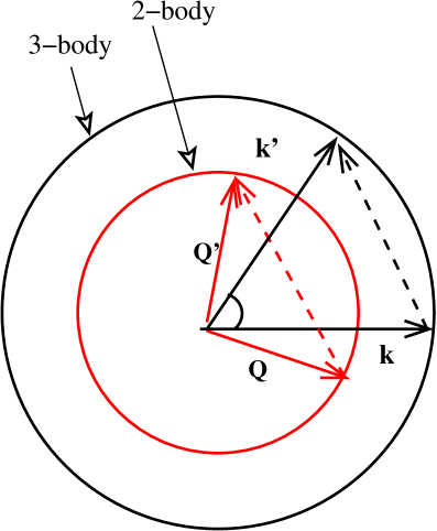
Figure 2: (Color online) Kinematics for the 3-body scattering in optimal factorization impulse approximation of Rihan. The lines and vectors have the same meaning as in Fig. 1.

Making use of Eqs. (31) and (23), the total scattering amplitude $F$ can be written in terms of the scattering amplitudes for each subsystem $f_{\cal I}$, where the normalization coefficients are

$${\cal N}_{1{\cal I}}=\left(\frac{\mu_{1,23}}{\mu_{1{\cal I}}}\right)^{2}\left(\frac{1}{\widehat{\cal C}_{1{\cal I}}}\right)^{2}~{}~{}~{},~{}~{}~{}{\cal I}=1,2~{}~{}.$$ (42)

We note that for small scattering angles the energy parameters reduce to Eqs. (29) and (27) and the normalization coefficients to Eq. (33).

III.1.3 The 3b on-shell FIA [Chew]

For completeness we discuss now the approximation discussed in Chew51 ; Chew50 , although no practical application will be made here. Within this approximation, the relative incident momenta between the subsystems $q_{23}$ is again neglected when compared with the incident projectile momentum. That is, setting $Q_{23}=0$ one gets

$$\vec{\cal Q}_{12}=\frac{\mu_{12}}{\mu_{1,23}}\vec{k}_{1}~{}~{}.$$ (43)

In addition, it is also assumed that

$$|\vec{\cal Q}\,^{\prime}_{12}|=|\vec{\cal Q}_{12}|~{}~{},~{}~{}|\vec{\kappa}|=|\vec{\Delta}|~{}.$$ (44)

The kinematics in the Chew approximation is represented schematically in Fig. 3.

The energy parameters, $\omega_{12}$ and $\omega_{13}$ are given by Eq. (27) and Eq. (29) respectively. By construction from these equations the matrix elements are on the energy shell. The normalization coefficients for the angular scattering amplitudes are identical to those derived in the KL approximation Eq. (33).

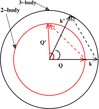
Figure 3: (Color online) Kinematics for the 3-body scattering in the on-shell impulse approximation of Chew. The lines and vectors have the same meaning as in Fig. 1.

III.1.4 The 3b on-shell FIA [Crespo and Johnson]

In this approach, followed in the most current applications of MST Cres99 ; Cres02 ; CresRNB , the initial internal relative momentum $q_{23}$ is neglected in the transition matrix elements, and thus Eq. (43) is satisfied. In addition,

$$\vec{\cal Q}\,^{\prime}_{12}=\vec{\cal Q}_{12}+\vec{\Delta}$$ (45)

The energy parameters, $\omega_{12}$ and $\omega_{13}$ are given by Eq. (27) and Eq. (29) respectively.

The single-scattering terms can then be written as a function of the transition amplitude for proton-subsystem scattering and the density for the subsystem $\rho_{23}$,

$$T=\langle\frac{\mu_{12}}{\mu_{1,23}}\vec{k}\,_{1}+\vec{\Delta}|\hat{t}_{2}(\omega_{12})|\frac{\mu_{12}}{\mu_{1,23}}\vec{k}_{1}\rangle\rho_{23}\left(\frac{m_{3}}{M_{23}}\vec{\Delta}\right)$$

$$~{}~{}~{}+\langle\frac{\mu_{13}}{\mu_{1,23}}\vec{k}_{1}+\vec{\Delta}|\hat{t}_{3}(\omega_{13})|\frac{\mu_{13}}{\mu_{1,23}}\vec{k}_{1}\rangle\rho_{23}\left(\frac{m_{2}}{M_{23}}\vec{\Delta}\right)$$

(46)

or equivalently

$$T=\hat{t}_{2}(\omega_{12},\Delta,{\cal K}_{12},\phi)\rho_{23}\left(\frac{m_{3}}{M_{23}}\vec{\Delta}\right)$$

$$~{}~{}~{}+\hat{t}_{3}(\omega_{13},\Delta,{\cal K}_{13},\phi)\rho_{23}\left(\frac{m_{2}}{M_{23}}\vec{\Delta}\right)~{}~{},$$

(47)

with $\phi$ the angle between $\Delta$ and ${\cal K}$. On the energy shell, $\phi=\pi/2$. The matrix elements of the transition amplitude are half on the energy shell since ${\cal Q}_{12}=\sqrt{2\mu_{12}\omega_{12}}/\hbar$, but ${\cal Q}\,^{\prime}_{12}\neq{\cal Q}_{12}$, as represented schematicaly in Fig. 4.

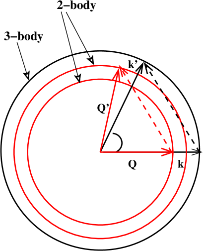
Figure 4: (Color online) Kinematics for the 3-body scattering in the off-energy shell, OFFES, impulse approximation. The lines and vectors have the same meaning as in Fig. 1.

This approach is however impractical if one has only on-shell scattering amplitudes for the scattering from the subsystems. This is the case, for example, when these amplitudes are obtained by fitting scattering data. We note that for small scattering angles, the scattering angle for projectile subsystem ${\cal I}=2$ scattering, $\theta_{12}$, satisfies

$$\theta_{1,2}\sim\frac{\mu_{1(23)}}{\mu_{1{2}}}\theta~{}~{}.$$ (48)

This means that the range of physical momentum transfers over which the on-shell $t_{12}$ transition amplitude is defined is smaller than the range of momentum transfers accessible in for the scattering from the 3-body system.

If the dependence of the transition amplitude $\hat{t}_{\cal I}(\omega_{1{\cal I}},\Delta,{\cal K}_{1{\cal I}},\phi)$ in Eq. (47) on the total momentum is assumed to be small then we can replace the matrix elements by their on-shell values at the appropriate energy. On the energy shell, the total momentum ${\cal K}$ is related to the momentum transfer $\Delta$, and $\phi=\pi/2$. In most current multiple scattering applications Cres99 ; Cres02 ; CresRNB the on-shell approximation is made within a partial wave expansion of the transition amplitude, but the angular direction is kept constant. We refer to this factorized impulse approximation approach as projected on-energy shell [POES].

Making use of Eq. (47) and Eq. (23) the total scattering amplitude $F$ can be written in terms of the scattering amplitudes for each subsystem $f_{\cal I}$, where the normalization coefficients are given as in Eq. (33).

III.2 The Fixed scatterer or adiabatic approximation [FSA]

Within the fixed scatterer or adiabatic approximation, the internal Hamiltonian between the clusters is taken to a constant $\bar{H}$, that is, the operator projectile-${\cal I}$ target subsystem transition amplitude $\tau_{\cal I}$ is replaced by

$$\tilde{t}_{\cal I}=v_{\cal I}+v_{\cal I}\tilde{G}_{0}\tilde{t}_{\cal I}$$ (49)

where $\tilde{G}_{0}$

$$\tilde{G}_{0}=\left(E^{+}-K_{1}-\bar{H}\right)^{-1}~{}~{}.$$ (50)

Even after this simplification, the solution of this problem involves the solution of a system of coupled equations, which in practice requires truncation of the angular momenta in order to make the problem solvable Chr97 . A notable simplification of the problem is achieved in general when one neglects the interaction of the projectile with all the fragments except the core Ron97b ; Cres99 , the so called core-recoil model. In this particular case, the few-body problem can be exactly solved, leading to a simple factorized expression, the product of the transition amplitude for the scattering from the core evaluated at the appropriate energy and a structure form factor.

Within the FSA framework for the case where the interaction between the projectile and fragment 3 is neglected the total transition amplitude takes the form,

$$T^{\rm FSA}=\langle\vec{k}\,^{\prime}_{1}|\tilde{t}_{2}(E)|\vec{k}_{1}\rangle\rho_{23}\left(\frac{m_{3}}{M_{23}}\vec{\Delta}\right)~{}~{}.$$ (51)

We note that in the FSA approach, the energy parameter is $E=\hbar k_{1}^{2}/2\mu_{1,23}$ and thus, a distinctive feature of the FSA is that the two-body amplitude is calculated with the reduced mass $\mu_{1,23}$, instead of the reduced mass appropriate for the two-body scattering which appears in the FIA scattering amplitude. In the general case, i.e., when the interaction with the two target subsystems is considered, one can perform a multiple scattering expansion of the few-body amplitude in terms of the individual T-matrices $\tilde{t}_{\cal I}$ for the fragments which, in leading order, yields the factorized expression,

$$T^{\rm FSA}=\langle\vec{k}\,^{\prime}_{1}|\tilde{t}_{2}(E)|\vec{k}_{1}\rangle\rho_{23}\left(\frac{m_{3}}{M_{23}}\vec{\Delta}\right)$$

$$~{}~{}~{}+\langle\vec{k}\,^{\prime}_{1}|\tilde{t}_{3}(E)|\vec{k}_{1}\rangle\rho_{23}\left(\frac{m_{2}}{M_{23}}\vec{\Delta}\right)~{}~{},$$ (52)

In principle, the fixed scatterer approximation is conceptually different from the factorized impulse approximation, in any of the versions discussed above. However,we shall show further down that in the high energy limit, the calculated elastic scattering observables using the FSA and the FIA (POES or Rihan) are essentially identical. The formal relation between the FSA and FIA and their relation with the Glauber theory will be explored elsewhere.

IV The single scattering 4-body problem

We consider now the case of proton scattering from a nucleus assumed to be well described by a three body model (for example ¹¹Li), as a core (here labeled as subsystem 4) and two valence weakly bound systems (subsystems 2 and 3). Neglecting core excitation, the target wave function is

$$\Phi(\vec{r},\vec{R},{\xi}_{4})=\left[\phi_{23,4}(\vec{r},\vec{R})\otimes\varphi_{4}(\xi_{4})\right]~{}~{},$$ (53)

where $\varphi_{4}(\xi_{4})$ is the core internal wave function and $\phi_{23,4}(\vec{r},\vec{R})$ the three body valence wave function relative to the core. The internal degrees of freedom of the core are denoted globally as $\xi_{4}$. The total transition amplitude is then

$$T^{IA} = \langle\vec{k}\,^{\prime}_{1}\Phi|\hat{t}_{12}|\vec{k}_{1}\Phi\rangle+\langle\vec{k}\,^{\prime}_{1}\Phi|\hat{t}_{13}|\vec{k}_{1}\Phi\rangle+\langle\vec{k}\,_{1}\Phi|\hat{t}_{14}|\vec{k}_{1}\Phi\rangle$$ (54)

$$+ \cdots$$

where within the single scattering approximation only the first three terms are taken into account. We first consider the situation where particle 1 scatters from one of the valence systems, named subsystem 2. The relevant Jacobian coordinates are

$$\vec{q}_{1,2} = \frac{m_{2}\vec{k}_{1}-m_{1}\vec{k}_{2}}{M_{12}}$$ (55)

$$\vec{q}_{2,3} = \frac{m_{3}\vec{k}_{2}-m_{2}\vec{k}_{3}}{M_{23}}$$ (56)

$$\vec{q}_{23,4} = \frac{m_{4}\vec{P}_{23}-M_{23}\vec{k}_{4}}{M_{234}}~{}~{},$$ (57)

where $\vec{P}_{12}=\vec{k}_{1}+\vec{k}_{2}$, $\vec{P}_{34}=\vec{k}_{3}+\vec{k}_{4}$, etc. In the center of mass of the total four-body system, $\vec{\cal P}_{t}=\sum_{i=1}^{4}\vec{k}_{i}=0$. The intermediate states propagator is given by

$$\hat{G}_{0}=\left(E^{+}-\frac{\hbar^{2}}{2\mu_{12}}\vec{q}^{\,2}_{\,12}-\frac{\hbar^{2}}{2\mu_{34}}\vec{q}^{\,2}_{\,34}-\frac{\hbar^{2}}{2\mu_{12,34}}\vec{q}^{\,2}_{\,12,34}\right)^{-1}$$ (58)

with

$$\vec{q}_{12,34} = \frac{M_{34}\vec{P}_{12}-M_{12}\vec{P}_{34}}{M_{1234}}$$ (59)

$$\vec{q}_{3,4} = \frac{m_{4}\vec{k}_{3}-m_{3}\vec{k}_{4}}{M_{34}}$$ (60)

and $\mu_{12}$, $\mu_{34}$, $\mu_{12,34}=M_{12}M_{34}/M_{1234}$ the appropriate reduced masses. Using the fact that the operator $\hat{t}_{12}$ is independent of the spatial variables of the core, the single scattering matrix elements are given by

$$\langle\vec{k}^{\prime}_{1}\phi_{23,4}|\hat{t}_{2}|\vec{k}_{1}\phi_{23,4}\rangle=\int\int d\vec{q}_{23}\,d\vec{q}_{23,4}\phi^{*}_{23,4}\left(\vec{q}_{23}-\frac{m_{3}}{M_{23}}\vec{\Delta},\vec{q}_{23,4}-\frac{m_{4}}{M_{234}}\vec{\Delta}\right)\langle\vec{q}\,^{\prime}_{1,{2}}|\hat{t}_{2}(\hat{\omega}_{1{2}})|\vec{q}_{1,2}\rangle\phi_{23,4}\left(\vec{q}_{23},\vec{q}_{23,4}\right)$$ (61)

The initial (and final) relative momentum between the projectile and the subsystem ${\cal I}=2$, $\vec{q}_{1,{2}}$ ($\vec{q}\,^{\prime}_{1,{2}}$) are respectively

$$\vec{q}_{1,{2}} = \frac{\mu_{12}}{\mu_{1,234}}\vec{k}_{1}-\frac{\mu_{12}}{m_{2}}\left[\vec{q}_{23}+\frac{m_{2}}{M_{23}}\vec{q}_{23,4}\right]$$

$$\vec{q}\,^{\prime}_{1,{2}} = \frac{\mu_{12}}{\mu_{1,234}}\vec{k}\,^{\prime}_{1}-\frac{\mu_{12}}{m_{2}}\left[\vec{q}\,^{\prime}_{23}+\frac{m_{2}}{M_{23}}\vec{q}\,^{\prime}_{23,4}\right]$$ (62)

$$= \frac{\mu_{12}}{\mu_{1,234}}\vec{k}\,^{\prime}_{1}-\frac{\mu_{12}}{m_{2}}\left[\vec{q}_{23}+\frac{m_{2}}{M_{23}}\vec{q}_{23,4}\right]$$

$$- \frac{\mu_{12}}{m_{2}}\left[\frac{m_{3}}{M_{23}}+\frac{m_{2}}{M_{23}}\frac{m_{4}}{M_{234}}\right]\vec{\Delta}~{}~{},$$

with $\alpha_{12}=\mu_{12}/m_{2}$ defined as in the 3-body case. The energy parameter $\hat{\omega}_{1{2}}$ is

$$\hat{\omega}_{12} = E-\frac{\hbar^{2}}{2\mu_{34}}\left[\frac{m_{3}M_{234}}{M_{23}M_{34}}\vec{q}_{23,4}-\frac{m_{4}}{M_{34}}\vec{q}_{23}\right]^{\,2}$$

$$- \frac{\hbar^{2}}{2\mu_{12,34}}\left[\frac{M_{34}}{M_{234}}\vec{k}_{1}+\frac{m_{2}}{M_{23}}\vec{q}_{23,4}+\vec{q}_{23}\right]^{\,2}$$

We note that expressions Eq. (62) and Eq. (LABEL:fullfoldingE4b) reduce to the 3-body problem in the limit where we take $m_{4}=0$.

We now consider the situation where particle 1 scatters from the core named subsystem 4. The relevant Jacobian coordinates are $\vec{q}_{2,3},\vec{q}_{23,4}$ and

$$\vec{q}_{1,4} = \frac{m_{4}\vec{k}_{1}-m_{1}\vec{k}_{4}}{M_{14}}~{}~{}.$$ (64)

The intermediate states propagator is given by

$$\hat{G}_{0}=\left(E^{+}-\frac{\hbar^{2}}{2\mu_{14}}\vec{q}^{\,2}_{\,14}-\frac{\hbar^{2}}{2\mu_{23}}\vec{q}^{\,2}_{\,23}-\frac{\hbar^{2}}{2\mu_{14,23}}\vec{q}^{\,2}_{\,14,23}\right)^{-1}~{}~{},$$ (65)

with

$$\vec{q}_{14,23}=\frac{M_{23}\vec{P}_{14}-M_{14}\vec{P}_{23}}{M_{1234}}$$ (66)

and $\mu_{14}$, $\mu_{23}$, $\mu_{14,23}=M_{14}M_{23}/M_{1234}$ the appropriate reduced masses. The single scattering matrix elements for the scattering from the core

$$\langle\vec{k}^{\prime}_{1}\phi_{23}\phi_{4}|\hat{t}_{4}|\varphi_{4}\phi_{23,4}\vec{k}_{1}\rangle=\int\int d\vec{q}_{23}\,d\vec{q}_{23,4}\phi^{*}_{23,4}\left(\vec{q}_{23},\vec{q}_{23,4}+\frac{M_{23}}{M_{234}}\vec{\Delta}\right)\langle\vec{q}\,^{\prime}_{1,{4}}\phi_{4}|\hat{t}_{4}(\hat{\omega}_{1{4}})|\varphi_{4}\vec{q}_{1,4}\rangle\phi_{23,4}\left(\vec{q}_{23},\vec{q}_{23,4}\right)$$ (67)

The initial (and final) relative momentum between the projectile and the subsystem ${\cal I}=4$, $\vec{q}_{1,4}$ ($\vec{q}\,^{\prime}_{1,4}$) are respectively

$$\vec{q}_{1,4} = \frac{\mu_{14}}{\mu_{1,234}}\vec{k}_{1}+\frac{\mu_{14}}{m_{4}}\vec{q}_{23,4}~{}~{},$$

$$\vec{q}\,^{\prime}_{1,{4}} = \frac{\mu_{14}}{\mu_{1,234}}\vec{k}\,^{\prime}_{1}+\frac{\mu_{14}}{m_{4}}\vec{q}\,^{\prime}_{23,4}~{}~{}.$$ (68)

The energy parameter $\hat{\omega}_{14}$ is

$$\omega_{14}=E-\frac{\hbar^{2}}{2\mu_{23}}q_{23}^{\,2}-\frac{\hbar^{2}}{2\mu_{14,23}}\left[\frac{M_{23}}{M_{234}}\vec{k}_{1}-\vec{q}_{23,4}\right]^{\,2}~{}~{}.$$ (69)

In the limit where we take $m_{3}=0$, these equations reduce to the 3-body case. As in the 3-body case, it is desirable to obtain after suitable approximations a factorized expression of the transition amplitude matrix elements and the target form factor

$$\rho_{23,4}(\vec{\Delta}_{1},\vec{\Delta}_{2}) = \int d\vec{Q}_{1}d\vec{Q}_{2}\,\phi^{*}_{23,4}(\vec{Q}_{1}+\vec{\Delta}_{1},\vec{Q}_{2}+\vec{\Delta}_{2})$$ (70)

$$\times \phi_{23,4}(\vec{Q}_{1},\vec{Q}_{2})~{}~{}~{}~{}.$$

In here $\phi_{23,4}(\vec{Q}_{1},\vec{Q}_{2})$ is the Fourier transform of the wave function of the two body valence system relative to the core $\phi_{{}_{23,4}}(\vec{r},\vec{R})$. The factorized impulse approximation expression for the 4-body case is

$$T^{\rm FIA} = \langle\vec{\cal Q}\,^{\prime}_{12}|\hat{t}_{2}(\omega_{12})|\vec{\cal Q}_{12}\rangle\rho_{23,4}\left(\frac{m_{3}}{M_{23}}\vec{\Delta},\frac{m_{4}}{M_{234}}\vec{\Delta}\right)$$

$$+ \langle\vec{\cal Q}\,^{\prime}_{13}|\hat{t}_{3}(\omega_{13})|\vec{\cal Q}_{13}\rangle\rho_{23,4}\left(\frac{m_{2}}{M_{23}}\vec{\Delta},\frac{m_{4}}{M_{234}}\vec{\Delta}\right)$$

$$+ \langle\vec{\cal Q}\,^{\prime}_{14}\phi_{4}|\hat{t}_{4}(\omega_{14})|\phi_{4}\vec{\cal Q}_{14}\rangle\rho_{23,4}\left(0,\frac{M_{23}}{M_{234}}\vec{\Delta}\right)$$

where $\vec{\cal Q}$ and $\omega$ are the appropriate relative momenta and energy parameter respectively to be discussed bellow, which are a generalization of the 3 body case.

IV.0.1 The 4b on-shell FIA [Kujawski and Lambert]

Within this approximation, the relative momenta between the subsystems $q_{23}$ and $q_{23,4}$ are neglected when compared with the incident projectile momenta in the matrix elements of the projectile subsystem transition matrix elements whenever they appear, that is,

$$|\vec{Q}_{23}|=|\vec{Q}\,^{\prime}_{23}|=0$$

$$|\vec{Q}_{23,4}|=|\vec{Q}\,^{\prime}_{23,4}|=0~{}~{}.$$ (72)

From Eq. (62) one obtains for the relative momenta between the projectile and subsystem ${\cal I}=2$

$$\vec{\cal Q}_{12}=\frac{\mu_{12}}{\mu_{1,234}}\vec{k}_{1}~{}~{},~{}~{}\vec{\cal Q}\,^{\prime}_{12}=\frac{\mu_{12}}{\mu_{1,234}}\vec{k}\,^{\prime}_{1}$$ (73)

and for the energy parameter

$$\omega_{12}=\frac{\mu_{1{2}}}{\mu_{1,234}}E$$ (74)

and similarly for the scattering from subsystems ${\cal I}=3,4$. The single scattering terms can then be written as

$$T=\langle\frac{\mu_{14}}{\mu_{1,234}}\vec{k}\,^{\prime}_{1}|\hat{t}_{4}(\omega_{14})|\frac{\mu_{14}}{\mu_{1,234}}\vec{k}_{1}\rangle\rho_{23,4}\left(0,\frac{m_{23}}{M_{234}}\vec{\Delta}\right)$$

$$+ \langle\frac{\mu_{12}}{\mu_{1,234}}\vec{k}\,^{\prime}_{1}|\hat{t}_{2}(\omega_{12})|\frac{\mu_{12}}{\mu_{1,234}}\vec{k}_{1}\rangle\rho_{23,4}\left(\frac{m_{3}}{M_{23}}\vec{\Delta},\frac{m_{4}}{M_{234}}\vec{\Delta}\right)$$

$$+ \langle\frac{\mu_{13}}{\mu_{1,234}}\vec{k}\,^{\prime}_{1}|\hat{t}_{3}(\omega_{13})|\frac{\mu_{13}}{\mu_{1,234}}\vec{k}_{1}\rangle\rho_{23,4}\left(\frac{m_{2}}{M_{23}}\vec{\Delta},\frac{m_{4}}{M_{234}}\vec{\Delta}\right)~{}~{}.$$

By construction, from Eqs. (73-74) the matrix elements of the transition amplitudes are on-shell.

As in the three-body case the total scattering amplitude, $F$, can be written in terms of the scattering amplitudes for each subsystem $f_{\cal I}$, where the normalization coefficients are

$${\cal N}_{1{\cal I}}=\left(\frac{\mu_{1,234}}{\mu_{1{\cal I}}}\right)^{2}~{},~{}{\cal I}=2,3,4$$ (76)

IV.0.2 The 4b on-shell FIA [Rihan]

The extension of the optimal factorized approximation discussed in the work of Rihan Rih77 ; Rih96 to the four-body problem is straightforward. The relative momentum between the subsystems is taken to the mid-point value where the product of the wave function peaks. For the scattering from subsystem ${\cal I}=2$ this yields

$$\vec{Q}_{23} = \frac{1}{2}\frac{m_{3}}{M_{23}}\vec{\Delta}$$

$$\vec{Q}_{23,4} = \frac{1}{2}\frac{m_{4}}{M_{234}}\vec{\Delta}~{}~{},$$ (77)

which leads to

$$\vec{\cal Q}_{1,{2}} = \hat{\beta}_{12}\vec{k}_{1}-\frac{\alpha_{12}\hat{\gamma}_{12}}{2}\vec{\Delta}~{}~{},$$ (78)

with $\alpha_{12}$ defined as in the three-body case and $\hat{\beta}_{12}=\mu_{12}/\mu_{1,234}$, $\hat{\gamma}_{12}=M_{34}/M_{234}$. Note that these expressions reduce to the 3-body case in the limit where we take $m_{4}=0$. Since this approximation involves on-shell matrix elements the energy parameter can be evaluated as

$$\omega_{12}=\frac{\hbar^{2}}{2\mu_{12}}|\vec{{\cal Q}}_{12}|^{2}=E\frac{\mu_{12}}{\mu_{1,234}}\widehat{\cal C}_{12}$$ (79)

with

$$\widehat{\cal C}_{12}=\left[\frac{\mu_{1,234}}{\mu_{12}}\right]^{2}[1+{\cal C}_{12}+{\cal C}_{12}\,\cos\theta]~{}~{},$$ (80)

where $\theta$ is the scattering angle and

$${\cal C}_{12} = -\alpha_{12}\hat{\gamma}_{12}+\frac{1}{2}\alpha_{12}^{2}\hat{\gamma}_{12}^{2}~{}~{}.$$ (81)

The normalization factor is formally identical to the three-body case, Eq. (42), with $\widehat{\cal C}_{12}$ replaced by Eq. (80). Similar expressions can be derived for the case of the scattering from subsystem ${\cal I}=3$. In the case of the scattering from subsystem ${\cal I}=4$, the optimal approximation prescribes

$$\vec{Q}_{23} = 0$$

$$\vec{Q}_{23,4} = -\frac{1}{2}\frac{M_{23}}{M_{234}}\vec{\Delta}$$ (82)

which leads to

$$\vec{\cal Q}_{1,4} = \frac{\mu_{14}}{\mu_{1,234}}\vec{k}_{1}-\frac{\mu_{14}}{m_{4}}\frac{1}{2}\frac{M_{23}}{M_{234}}\vec{\Delta}$$ (83)

$$= \hat{\beta}_{14}\vec{k}_{1}-\frac{\alpha_{14}\hat{\gamma}_{14}}{2}{\vec{\Delta}}$$

with $\hat{\beta}_{14}=\frac{\mu_{14}}{\mu_{1,234}}$, $\hat{\gamma}_{14}=M_{23}/M_{234}$ and for the energy parameter,

$$\omega_{14}=\frac{\hbar^{2}}{2\mu_{14}}{\cal Q}_{14}^{2}=E\frac{\mu_{14}}{\mu_{1,234}}\widehat{\cal C}_{14}$$ (84)

with

$$\widehat{\cal C}_{14}=\left[\frac{\mu_{1,234}}{\mu_{14}}\right]^{2}\left[1+{\cal C}_{14}+{\cal C}_{14}\,\cos\theta\right]$$ (85)

where

$${\cal C}_{14}=-\alpha_{14}\hat{\gamma}_{14}+\frac{1}{2}\alpha_{14}^{2}\hat{\gamma}_{14}^{2}~{}~{}.$$ (86)

IV.0.3 The 4b on-shell FIA [Crespo and Johnson]

In this approach the initial relative momenta $q_{23},q_{23,4}$ are neglected in the transition matrix elements momentum transfer. For the scattering of subsystem ${\cal I}=2$

$$\vec{\cal Q}_{12}=\frac{\mu_{12}}{\mu_{1,234}}\vec{k}_{1}~{}~{},~{}~{}\vec{\cal Q}\,^{\prime}_{12}=\vec{\cal Q}_{12}+\vec{\Delta}$$ (87)

and similarly for the scattering of the other subsystems.

V The ⁶He structure model

The ⁶He is here described as a three-body system $n$+$n$+⁴He. The bound wave functions are obtained by solving the Schrödinger equation in hyperspherical coordinates. We consider two structure models defined in terms of different effective 3-body (3B) potentials, which are introduced to overcome the underbinding caused by the other closed channels, most important of which the $t$+$t$ breakup. In both models the $n$-⁴He potential is taken from Ref. Bang79 ; Tho00 , and use the GPT $NN$ potential gpt with spin-orbit and tensor components. In the first model (R5) of Dan98 the 3B effective potential in the hyperspherical coordinates is given as a function of the hyperradius $\rho$

$$V^{(R5)}(\rho)=\frac{-V_{3}}{1+(\hat{\rho}/5)^{3}}~{}~{}.$$ (88)

In the second model (R2) of Tim00 the potential is defined as

$$V^{(R2)}(\rho)=-U_{3}\exp(-\hat{\rho}^{3})~{}~{}.$$ (89)

In these equations $\hat{\rho}=\rho/\rho_{0}$, where $\rho_{0}$= 5 fm and 1 fm for R5 and R2 respectively. The strength of the 3B effective potential is tuned to reproduce the experimental three-body separation energy, with V₃=–1.60 MeV and U₃=–293.5 MeV. The models R5 and R2 predict, with an $\alpha$ particle rms matter radius of 1.49 fm, ⁶He rms matter radii of 2.50 fm and 2.35 fm respectively.

VI Results

In this section we evaluate the elastic scattering differential cross section for the scattering of protons on ⁶He at $E_{\rm lab}=717$ MeV within the four-body FIA single scattering approximation and Fixed scatterer approximation FSA. In the case under study, the single scattering terms involves contributions from the valence nucleons and from the ⁴He core.

VI.1 p+cluster

In the factorized impulse approximations discussed in the present work, the total T-matrix is expressed in terms of the on-shell matrix elements of the two-body amplitudes evaluated at an appropriate momentum transfer and energy. The $NN$ on-shell scattering amplitudes were obtained from a realistic $NN$ Paris interaction, as in Cres99 ; Cres02 ; CresRNB .

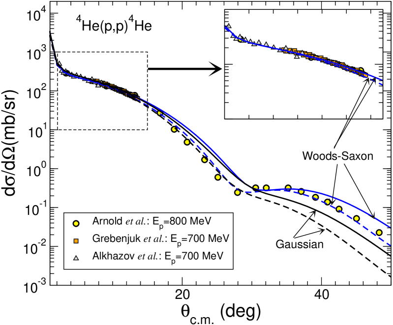
Figure 5: (Color online) Calculated elastic scattering for $p+^{4}$He at $E_{p}$=700 MeV (solid lines) and 800 MeV (dashed lines), using a Gaussian and a Woods-Saxon parametrization as described in the text. The data are taken from Refs. Alk97 ; Greb89 ; Arn79

.

The two-body scattering amplitude for the scattering $p+^{4}$He was calculated with a phenomenological optical potential, with parameters obtained by fitting existing data for the elastic scattering $p+^{4}$He at $E_{\rm p}=700$ MeV Alk97 ; Greb89 and 800 MeV Arn79 . We consider two different parametrizations for the $p+\alpha$ optical potential. In the first one, based on the work of Baldini-Neto et al. Bal03 we take the optical potential as a sum of two terms, real and imaginary, of Gaussian shape

$$U(r)=V_{0}{\cal F}(r,r_{0})+iW_{0}{\cal F}(r,r_{i})$$ (90)

with ${\cal F}(r,r_{x})=\exp(-r^{2}/r_{x}^{2})$. The values of the radii and the real and imaginary depths were adjusted simultaneously in order to minimize the $\chi^{2}$ with the experimental data. These fits were performed with the computer code FRESCO Thom88 , version frxy. The final values of these parameters where $V_{0}$=+73 MeV, $r_{0}$=1.37 fm, $W_{0}$=-162 MeV and $r_{i}$=1.32 fm.

We have also taken a phenomenological potential of Woods-Saxon (WS) shape, i.e.:

$$U(r)=V_{0}f(r,r_{0},a_{0})+iW_{i}f(r,r_{i},a_{i})$$ (91)

with $f(r,r_{x},a_{x})=[1+\exp[(r-R_{x})/a_{x}]^{-1}$, where $R_{x}=r_{x}A^{1/3}$.

To reduce the number of degrees of freedom in the best fit search we constrained the parameters to $r_{0}$=$r_{i}$ and $a_{0}$=$a_{i}$. With this condition, a best-fit analysis of the data yields the values $V_{0}$=+72 MeV, $W_{i}$=-115 MeV, $r_{0}$=$r_{i}$=1.14 fm, and $a_{0}$=$a_{i}$=0.31 fm. Note that with both geometries the real potential was positive in our fits, indicating a dominance of the repulsive part in the $p+^{4}$He interaction at these energies. The data and calculated differential elastic cross sections obtained with these parametrized potentials for $p+^{4}$He at $E_{p}$=700 and 800 MeV are shown in Fig. 5. The solid and dashed lines, corresponding to $E_{p}$=700 MeV and 800 MeV respectively, reproduce very well the forward scattering data for both the Gaussian and Woods Saxon parametrization. By contrast, the calculated differential cross section tends to deviate from the data of Arn79 at larger angles in the case of the Gaussian parametrization. The WS optical model improves the fit in this angular region.

VI.2 $p+^{6}$He

The two-body $NN$ and $p+\alpha$ scattering amplitudes obtained by fitting elastic data are now used to evaluate the total transition amplitude for $p+^{6}$He scattering.

The Coulomb interaction was included in an approximate way as summarized in appendix A. The elastic scattering observables shown in here were evaluated using relativistic kinematics as discussed in detail in appendix B. The relativistic kinematic effects nevertheless were found to be small.

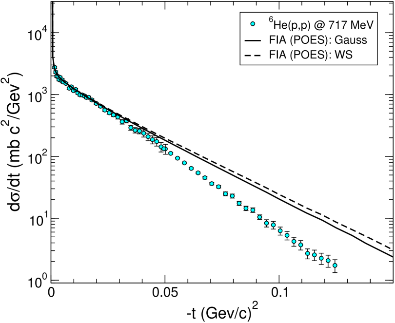
Figure 6: (Color online) Calculated $p+^{6}$He elastic scattering at 717 MeV for two different optical potentials for $p+^{4}$He. The data is taken from Aks02 ; Ege02 ; Aks03 .

In Fig. 6 we study the dependence of the calculated differential cross section for $p+^{6}$He elastic scattering with respect to the underlying $p+^{4}$He optical potential as a function of the squared four momentum transfer $-t=\Delta^{2}$. The solid and dashed lines represent the FIA-POES calculation using the Gaussian and WS Optical model parametrizations for core scattering. At higher momentum transfers the WS calculation gives a slightly bigger reduction of the cross section. The difference with respect to the Gaussian parameterization is small, and both parametrizations predict essentially the same differential cross section. The conclusions of the present work are therefore essentially independent of the underlying OM potential for the scattering from the core. We shall be using for definiteness the WS potential in all subsequent calculations.

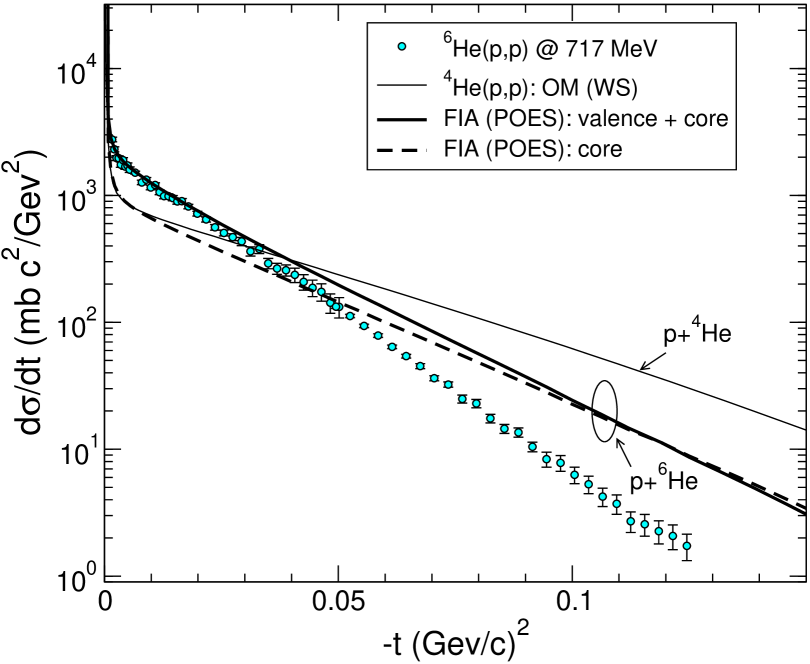
Figure 7: (Color online) Experimental and calculated $p+^{6}$He elastic scattering at 717 MeV within the FIA-POES approximation. For comparison purposes, the OM calculation for $p+^{4}$He elastic scattering, at the same energy per nucleon, is also included.

In Fig. 7, the thick solid line represents the calculated differential elastic cross section for $p+^{6}$He using the FIA-POES approximation. The dashed line was obtained neglecting the single scattering contribution from the valence neutrons. By comparing these two calculations, one finds that the core contribution dominates the large angle region but underpredicts the forward differential cross section. Also shown in the figure is the calculated elastic cross section for $p+^{4}$He (thin solid line). For values of $-t<0.03$ (GeV/c)² ($\theta_{\mathrm{c.m.}}<11^{\circ}$) the calculated $p+^{6}$He cross section is significantly bigger than the $p+^{4}$He cross section, providing a good agreement with the experimental data. Comparison of the two FIA calculations indicate that this enhancement on the cross section is mostly due to the presence of the valence neutrons, since the FIA calculation with core contribution alone is very close to the $p+^{4}$He distribution at these angles.

By contrast, for larger values of momentum transfer, the few-body calculation is smaller than the $p+^{4}$He curve. One notes from the figure that the two FIA calculations (core and core+valence single scattering) are very close to each other at large momentum transfer, indicating that, at least within the single scattering approximation, the depletion of the cross section at larger angles is mostly a consequence of core recoil effects. Although the experimental $p+^{6}$He data exhibit a depletion of the cross section with respect to the $p+^{4}$He distribution, the reduction predicted by the FIA calculation is too small to explain the data.

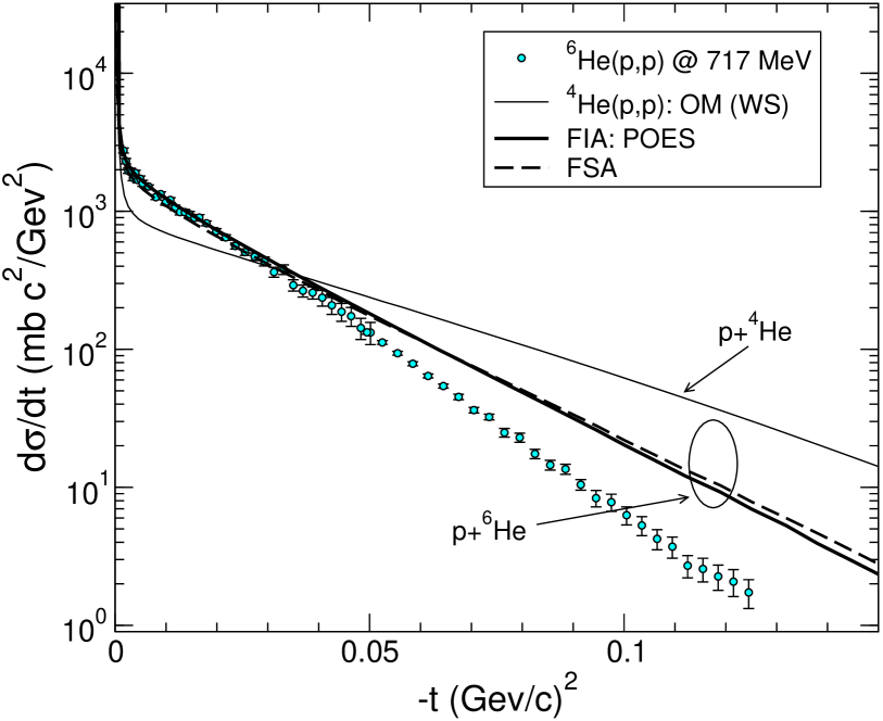
Figure 8: (Color online) Experimental and theoretical $p+^{6}$He elastic scattering at 717 MeV per nucleon, for several scattering models discussed in the text. The calculated $p+^{4}$He elastic distribution is included for comparison.

In Fig. 8 we compare the calculated $p+^{6}$He cross section using the FIA-POES (thick solid line), the FIA-KL (dashed-dotted line) and the FSA (adiabatic) approximation (long dashed). The cross section calculated with the FIA-Rihan approximation is very similar with the FIA-POES and therefore it is omitted from the figure. The difference between the predicted differential cross sections largely reflects the different rms matter radii.

The calculated differential cross section using FIA (POES and Rihan) and FSA are very similar. The elastic scattering observable calculated using the KL impulse approximation decays more slowly and the agreement with the data is comparatively even poor at the large angle region.

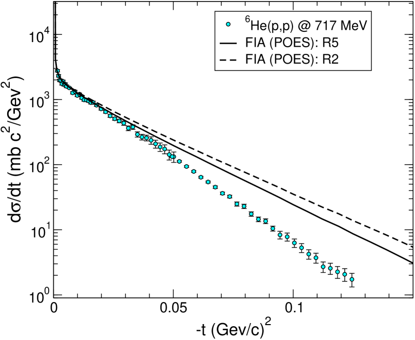
Figure 9: (Color online) Experimental and calculated $p+^{6}$He elastic scattering at 717 MeV for two different models for the ⁶He ground state.

We now study the sensitivity of the results with respect to the ⁶He wavefunction. In particular, we compare in Fig. 9 the FIA-POES calculations obtained with the R5 (thick solid line) and R2 (dashed line) ⁶He models discussed in section V. Both models give nearly identical results at low momentum transfer, but the R5, having a larger radius than R2, exhibits a larger reduction of the cross section at large scattering angles. However, these differences do not appear to explain the disagreement between the calculations and the data, and are much smaller than the differences obtained when using different scattering approximations.

From the analysis presented in this section, we can conclude that the factorized impulse approximations, in the different versions here presented, describe fairly well the elastic scattering data for $p+^{6}$He at small momentum transfer. In particular, they all show an increase of the cross section with respect to the $p+^{4}$He scattering, showing the effect of the valence neutrons on the elastic scattering. At momentum transfers above 0.05 (GeV/c)² all the calculations tend to overestimate the data, irrespective of the structure model used.

VII Conclusions

In this work we have reviewed and compared several approaches for the scattering of a nucleus by a weakly bound composite, based on the multiple scattering expansion of the total scattering amplitude, namely, Factorized Impulse and Fixed Scatterer/Adiabatic Approximations.

The Factorized Impulse Approximation (FIA) neglects the inter-cluster interaction and approximates the relative momentum between the loosely bound clusters. As for the Fixed Scatterer approximation (FSA) it replaces the internal Hamiltonian by a constant.

As a common feature, all these approaches express the single-scattering term as a product of a two-body scattering amplitude for the scattering of the fragment times a structure formfactor, which depends on the internal wavefunction of the composite system. This factorized form provides a simple interpretation of the scattering observable, by separating the role of the structure from the reaction dynamics.

These approaches have been then applied to the scattering of ⁶He on protons at $E$=717 MeV per nucleon, using $p$-$n$ amplitudes derived from a realistic $NN$ potential, and $p+^{4}$He amplitudes obtained from an optical model fit of existing elastic data. All the approximations here succeed in reproducing the $p+^{6}$He elastic data at small scattering angles. We found it crucial to include the effect of the valence neutrons to the single scattering contributions in order to explain the increase of the cross sections with respect to the $p+^{4}$He elastic data at the same energy per nucleon. At larger angles, both FSA and FIA calculations tend to overestimate the data.

This disagreement at larger angles could be traced to the neglect of higher order terms in the T-matrix expansion and will be discussed elsewhere.

Appendix A Treatment of the Coulomb Potential

The elastic differential angular distribution is evaluated from the total scattering amplitude

$$F^{\rm FIA} = {\cal N}_{12}^{1/2}\hat{f}_{2}(\omega_{12},\vec{\kappa}_{12})\rho_{23,4}\left(\frac{m_{3}}{M_{23}}\vec{\Delta},\frac{m_{4}}{M_{234}}\vec{\Delta}\right)$$

$$+ {\cal N}_{13}^{1/2}\hat{f}_{3}(\omega_{13},\vec{\kappa}_{13})\rho_{23,4}\left(\frac{m_{2}}{M_{23}}\vec{\Delta},\frac{m_{4}}{M_{234}}\vec{\Delta}\right)$$

$$+ {\cal N}_{14}^{1/2}\hat{f}_{4}(\omega_{14},\vec{\kappa}_{14})\rho_{23,4}\left(0,\frac{M_{23}}{M_{234}}\vec{\Delta}\right)~{}~{}.$$

In this equation, the scattering amplitude from the core includes the Coulomb interaction. The central scattering amplitude is taken as

$$\hat{f}^{c}_{4}(\theta) = f^{pt}_{C}(\theta)$$ (93)

$$+ \frac{1}{Q_{14}}\sum_{L}\exp(2i\sigma_{L})[(L+1)T_{4}^{L+}(N)$$

$$+ ~{}~{}~{}~{}~{}~{}~{}~{}~{}~{}~{}LT_{4}^{L-}(N)]P_{L}(\cos\theta)~{}~{}.$$

In Eq. (93), $f^{pt}_{C}(\theta)$ is the Coulomb scattering amplitude due to a point charge $Z_{4}e$ and $Q_{14}$ is the asymptotic projectile-core wave number. The $T_{4}^{L\pm}(N)$ are defined according to

$$T_{4}^{L\pm}(N)=\frac{\exp\left[2i\delta_{4}^{L\pm}(N)\right]-1}{2i}~{}~{},$$ (94)

where $L\pm$ denotes the orbital and total angular momenta, $J=L\pm\frac{1}{2}$ and $\delta_{4}^{L\pm}(N)$ are the Coulomb modified phase shifts Crespo90 . It follows from Eqs. (LABEL:Ffactorized4b-93) that the point Coulomb scattering amplitudes appears multiplied by the structure form factor $\rho_{23,4}\left(0,\frac{M_{23}}{M_{234}}\vec{\Delta}\right)$. Although this is an approximate treatment of the Coulomb interaction, it will only have effects at very small projectile momentum transfer and therefore does not modify the conclusions of the present work.

Appendix B Relativistic kinematic effects

In this section we describe how the expressions of sections III and IV should be modified in order to take into account relativistic kinematics. For simplification we consider the 3-body case Eq. (18). Expressions can be straightforward generalized to the 4-body case. For simplicity, we shall take in this section $c=1$.

Within MST, the projectile-target scattering scattering amplitude is constructed from the projectile-subsystem scattering amplitude as described in the text. We shall discuss the relativistic kinematics for the scattering of both the composite and each subsystem.

Let us consider the elastic scattering of projectile labelled 1 with a target $A$ with rest mass $m_{1}$ and $m_{A}$ respectively,

$$1+A\rightarrow 1+A$$ (95)

In our case $A$ represents the composite (2+3) two-body system. In relativistic kinematics one introduces the Lorentz invariant Mandelstam variable $s_{1A}=(E_{1}+E_{A})^{2}$ Joa87 . The differential cross section for projectile-target with respect to the four momentum transfer $t_{1A}$ is related to the c.m. differential cross section as:

$$\frac{d\sigma}{dt_{1A}}=\frac{\pi}{k_{1}^{2}}\frac{d\sigma}{d\Omega}~{}~{},$$ (96)

where $t_{1A}=-|\Delta|^{2}=2k_{1}^{2}(\cos\theta_{\rm c.m.}-1)$ and $k_{1}$ the projectile momentum in the projectile-target CM frame, that can be obtained from the Mandelstam variable $s_{1A}$. The cross section is evaluated from the scattering amplitude, related to the matrix elements of the total transition amplitude according to Joa87

$$F = \frac{(2\pi^{2})^{4}}{\hbar v_{1}}k_{1}^{2}\frac{dk_{1}}{d\omega}\langle\vec{k}\,^{\prime}_{1}|T(\omega)|\vec{k}_{1}\rangle~{}~{},$$ (97)

with $\omega=\sqrt{s_{1A}}-m_{1}-m_{A}$.

Let us now consider now the projectile scattering from subsystem ${\cal I}=2$. As before, one introduces the Mandelstam variable for the interacting pair $s_{12}$. For simplification, we shall take the relative momentum of the interacting pair $q_{23}$ nonrelativistically. We shall consider in here the two situations where $q_{23}=0$ (as in KL and POES impulse approximation) and $q_{23}\neq 0$ (as in optimal approximation discussed by Rihan)

• In the former case, in the laboratory frame $k_{2}=k_{3}=0$ and the Mandelstam variable $s_{12}$ can be readily evaluated

  $$s_{12}={m}_{1}^{2}+{m}_{2}^{2}+2{m}_{2}({m}_{1}+T_{1}^{\rm Lab})~{}~{}.$$ (98)

• In the later case, where $\vec{q}_{23}=\frac{1}{2}\frac{m_{3}}{M_{23}}\vec{\Delta}$, it is more convenient to evaluate $s_{12}$ in the projectile-subsystem ${\cal I}=2$ CM frame. In this case,

  $$s_{12}=\left(\sqrt{m_{1}^{2}+\vec{k}_{1}^{2}}+\sqrt{m_{2}^{2}+\vec{k}_{2}^{2}}\right)^{2}-(\vec{k}_{1}+\vec{k}_{2})^{2}$$ (99)

  To evaluate $s_{12}$, one takes $k_{1}$ from the Mandelstam invariant $s_{1A}$. The last term gives

  $$(\vec{k}_{1}+\vec{k}_{2})^{2}=\frac{1}{2}\gamma_{12}^{2}k_{1}^{2}\left[1+\cos\theta_{\rm c.m.}\right]$$ (100)

  and

  $$k_{2}^{2}=k_{1}^{2}\left[\chi_{12}^{2}+\frac{1}{4}\gamma_{12}^{2}-\gamma_{12}\chi_{12}\cos\theta_{\rm c.m.}\right]$$ (101)

  where $\chi_{12}=m_{2}/M_{23}+\frac{1}{2}\gamma_{12}$

The differential cross section for the scattering from subsystem ${\cal I}$ with respect to the four momentum transfer $t_{12}$, is related to the c.m. differential cross section as:

$$\frac{d\sigma}{dt_{12}}=\frac{\pi}{{\cal Q}_{12}^{2}}\frac{d\sigma}{d\Omega}_{12}~{}~{},$$ (102)

where $t_{12}=-|\kappa_{12}|^{2}=2{\cal Q}_{12}^{2}(\cos\theta_{1,2}-1)$ and ${\cal Q}_{12}$ the projectile momentum in the projectile-subsystem CM frame that can be obtained from $s_{12}$. The elastic scattering amplitude is related to the T-matrix elements through:

$$f_{2}=\frac{(2\pi^{2})^{4}}{\hbar v_{1}}k_{1}^{2}\frac{dk_{1}}{d\omega_{12}}\langle{\cal\vec{Q}^{\prime}}_{12}|\hat{t}_{2}(\omega_{12})|{\cal\vec{Q}}_{12}\rangle~{}~{},$$ (103)

with $\omega_{12}=\sqrt{s_{12}}-m_{1}-m_{2}$   .

References

• [1] C. J. Joachain. Quantum collision theory. North-Holland, 1987.
• [2] E. O. Alt, P. Grassberger, and W. Sandhas. Phys. Rev., C 1:85, 1970.
• [3] A. C. Fonseca. Phys. Rev., C 30:35, 1984.
• [4] T. Matsumoto, E. Hiyama, K. Ogata, Y. Iseri, M. Kamimura, S. Chiba, and M. Yahiro. Phys. Rev., C 70:061601, 2004.
• [5] M. L. Goldberger and K. M. Watson. Collision Theory. John Wiley and Sons, New York, 1964.
• [6] K. M. Watson. Phys. Rev., 105:1338, 1957.
• [7] R. Crespo and R. C. Johnson. Phys. Rev. 60, 034007, 1999.
• [8] R. Crespo, I. J. Thompson, and A. A. Korsheninnikov. Phys. Rev., C 66, 2002.
• [9] R. Crespo. Proceedings of rnb5, 3-8 april 2000, divonne, france. Nucl. Phys., A701:429c, 2002.
• [10] E. Kujawski and E. Lambert. Ann. Phys., 81:591, 1973.
• [11] T. H. Rihan. Phys. Rev., D 1235:1235, 1977.
• [12] T. H. Rihan. Phys. Rev., C 53:2328, 1996.
• [13] G. F. Chew. Phys. Rev., 84:1057–1058, 1951.
• [14] G. F. Chew. Phys. Rev., 80:196, 1950.
• [15] J. A. Christley, J.S. Al-Khalili, J. A. Tostevin, and R. C. Johnson. Nucl. Phys., A 624:275, 1997.
• [16] R. C. Johnson, J. S. Al-Khalili, and J. A. Tostevin. Phys. Rev. Lett., 79:2771, 1997.
• [17] J. Bang and C. Gignoux. Nucl. Phys., A 313:119, 1979.
• [18] I. J. Thompson, B. V. Danilin, V. D. Efros, J. S. Vaagen, J. M. Bang, and M. V. Zhukov. Phys. Rev., C 61:24318, 2000.
• [19] P. Pires D. Gogny and R. de Tourreil. Phys. Lett., 32B:591, 1970.
• [20] B. V. Danilin, I. J. Thompson, M. V. Zhukov, and J. S. Vaagen. Nucl. Phys., A632:383, 1998.
• [21] N. K. Timofeyuk and I. J. Thompson. Phys. Rev., C 61:044608, 2000.
• [22] G. D. Alkhazov et al. Phys. Rev. Lett., 78:2313, 1997.
• [23] O. G. Grebenjuk, A. V. Khanadeev, G. A. Korolev, S. I. Manayenkov, J. Saudinos, G. N. Velichko, and A. A. Vorobyov. Nucl. Phys., A 500:637, 1989.
• [24] L. G. Arnold, B. C. Clark, and R. L. Mercer. Phys. Rev., C 19:917, 1979.
• [25] E. Baldini-Neto, B. V. Carlson, R. A. Rego, and M. S. Hussein. Nucl. Phys., A 724:345, 2003.
• [26] I. J. Thompson. Comp. Phys. Rep. 7, 167, 1988.
• [27] F. Aksouh. Ph.D. Thesis. Investigation of the core-halo structure of the neutron rich nuclei 6,8He by intermediate-energy elastic proton scattering at high momentum transfer. PhD thesis, 2002.
• [28] P. Egelhof. Invited talk presented at the International Symposium on Physics of Unstable Nuclei. Nucl. Phys., A 722:C254–C260, 2002.
• [29] F. Aksough et al. Proceedings of the 10th International Conference on nuclear reaction mechanisms, Varenna, 2003. Review of the University of Milano, Ricerca Scientifica ed educazione permanente, Suppl. 122, 2003.
• [30] R. Crespo and J. A. Tostevin. Phys. Rev. C 41, 2615, 1990.