Two models with rescattering for high energy heavy ion collisions

Abstract

The effects of hadronic rescattering in RHIC-energy Au+Au collisions are studied using two very different models to describe the early stages of the collision. One model is based on a hadronic thermal picture and the other on a superposition of parton-parton collisions. Operationally, the output hadrons from each of these models are used as input to a hadronic rescattering calculation. The results of the rescattering calculations from each model are then compared with rapidity and transverse momentum distributions from the RHIC BRAHMS experiment. It is found that in spite of the different points of view of the two models of the initial stage, after rescattering the observed differences between the models are mostly “washed out” and both models give observables that agree reasonably well with each other and experiment.

I Introduction

The main goal of studying relativistic heavy ion collisions at the RHIC accelerator is to obtain information about the early stage of the collision when matter is at its most hot and dense state. Since experimentally one detects hadrons which have undergone final-state rescattering before decoupling from the collision, it is of interest to use model calculations to seek to disentangle the hadronic rescattering effect that tend to wash out the information about the early state of matter in which we are most interested. Such a rescattering calculation was carried out for RHIC collisions assuming a simple thermal-like model to describe the early stage of the collision Humanic:2002b ; Humanic:2006a ; Humanic:2006b , but since this thermal model was so simple, it proved difficult to interpret the results for the initial stage. The present work improves on the previous study in two ways: 1) a more elaborate thermal-like model is used for the initial stage, and 2) a second initial-stage model based on a superposition of parton-parton collisions is also included in the study. The advantage of 1) is clearly to make the interpretation of the initial-stage results easier, and the advantage of 2) is to compare the results of the thermal-like model with a model from a very different point of view, i.e. partonic, to see if after rescattering identifiable features of the different initial-stage models survive. We thus hope to address, at least for these two models, to what extent rescattering washes out the information about the initial stage of the collision. Our comparisons will be made with the hadronic observables rapidity and transverse momentum distributions, and these in turn will be compared with those extracted from the RHIC BRAHMS experiment Peter 2003 ; Djamel 2004 , as well as other RHIC experiments.

Sections II, III, and IV describe the thermal model, parton model, and rescattering calculation method, respectively. Sections V and VI give results of coupling the rescattering calculation with the thermal and parton models, respectively, and of comparisons with the BRAHMS experiment. Section VII presents a discussion of the results.

II The thermal-like model

II.1 Overview

The thermal-like model that we use builds on the Bjorken picture of a high energy heavy ion reaction Bjorken:1983a . The two heavy ions pass through one another in a central collision, whereby both nuclei become highly excited and a color field of high energy density is created in the space between the two ions after the collision. Particles are produced, in part from the two original nuclei with a net-baryon number to insure baryon conservation and in part from the region between the two ions, a region with a near vanishing net baryon content. It is assumed here that the produced particles may be described as originating from three thermal source centers, corresponding to the two heavy ions and the energy field in between. The source centers are extended in rapidity space, in the present model each distributed over a Gaussian shaped rapidity probability density. All three source centers are assumed to have the same temperature, $T$, but may contribute different numbers of particles. The created particles are assumed to have energy distributions that follow the Boltzmann distribution. The thermal model presented below thus for each type of particle creates three pools of four-momentum vectors, each pool distributed in rapidity around a source center. The differential distributions are then created by a weighted sum over contributions from the three source centers, where the weights, $N_{C}$, are the number of four-momentum vectors (particles) from each center.

It is well documented from previous work Johanna etc , that particle ratios, in principle integrated over the entire phase space, are described very well by thermal statistical ensembles, but thermal models that give insight into differential distributions in rapidity, transverse mass or momentum are scarce. To allow for the non-thermal phenomenon of flow, observed by experiments, the thermally produced particles are here allowed to rescatter as they emerge.

The purpose of the exercise presented here, is to show such differential distributions, compare them with data and obtain some understanding as to the extent such a description can reproduce the main features of the observations.

II.2 Structure of the model

For a given particle (mass=$m$) and a given source-center (rapidity=$y_{C}$) the four-momentum vectors are created by four subsequent Monte Carlo routines. The first one chooses the rapidity $y_{G}$ of the local source as a deviation from $y_{C}$ via a Gaussian probability density distribution,

$$G(y_{G},y_{C})=\frac{1}{\sigma_{C}\sqrt{2\pi}}\exp{(-(y_{G}-y_{C})^{2}/2\sigma_{C}^{2})},$$ (1)

where $\sigma_{C}$ characterizes the width of the Gaussian distribution corresponding to the selected source-center. The four momentum is generated in the local source reference system by choosing the polar and azimuthal angles, $\theta_{B}$ and $\phi_{B}$, such that the polar angle is taken from a constant distribution in $\cos(\theta_{B})$ for $0<\theta_{B}<\pi$, and $\phi_{B}$ is evenly distributed from 0 to $2\pi$. The energy of the particle, E_B, is finally chosen according to a Boltzmann prescription,

$$B(E_{B},T)=\frac{E_{B}\sqrt{E_{B}^{2}-m^{2}}}{Tm^{2}K_{2}(m/T)}\exp{(-E_{B}/T)}.$$ (2)

The temperature is denoted $T$ and is a global parameter used for all particle types, source-centers, and local sources. The $K_{2}$ is a modified Bessel function Assimof . The four-momentum components ($E_{B}$, $p_{x}$, $p_{y}$, $p_{z}$) following from the above Monte Carlo choices are then Lorentz transformed to the laboratory system and the process started over again with a new choice of $y_{G}$.

Each particle thus originates with its four-momentum from its own local source reference system. If the width $\sigma_{C}$=0, the particles from source-center C, will represent particles from a spherically symmetric Boltzmann source in the source-center reference system. A certain number of particles, $N_{m,C}$ are generated from each source-center, respectively, and the collection of four-vectors then constitutes the model data for particle species $m$. The multiplicity density distribution is then obtained as the sum of three source-center contributions

$$dn/dy_{m}(y)=N_{m0}F_{m0}(y)+N_{m-}F_{m-}(y)+N_{m+}F_{m+}(y),$$ (3)

where $y$ is the laboratory rapidity and the F-functions follow from the computation as described above.

II.3 Parameters of the model

For a particle of mass $m$, the model has 10 parameters: the temperature $T$, the rapidities of the three source-centers $y_{+}$, $y_{0}$ and $y_{-}$, the widths of the three Gaussian distributions $\sigma_{+}$, $\sigma_{0}$ and $\sigma_{-}$, and the number of particles from each source-center $N_{+}$, $N_{0}$ and $N_{-}$. In this report only symmetric collisions, A+A, are considered, which impose four restrictions on the parameters,

$$y_{0}=0$$ (4)

$$y_{+}=-y_{-}$$ (5)

$$\sigma_{+}=\sigma_{-}$$ (6)

$$N_{m+}=N_{m-}$$ (7)

The temperature for the following is set at 200 MeV, but later in the report it is increased to 270 MeV. The $N_{mC}$ values (number of particles or multiplicities) are chosen for each $(m,C)$ combination. The ratio $N_{+}/N_{0}$ has a decisive influence on the shape of the predicted rapidity density distribution, $dn/dy$, and on the slope of the transverse spectra. The same holds true for the $y_{+}$, the $\sigma_{+}$ and $\sigma_{0}$. The parameters were determined by asking for a reasonable agreement with the proton $dn/dy$ distribution for Au+Au at $\sqrt{s}$=200 GeV per nucleon as measured by the BRAHMS collaboration Peter 2003 , in the expectation that the $y_{+}$, $\sigma_{+}$ and $\sigma_{0}$, determining the Gaussian distributions, would be useful for all the particle species considered, an expectation that was fulfilled.

The BRAHMS proton data show that $y_{+}$ is larger than 3.0, but they do not fix the value, because of the limited rapidity coverage of the experiment. The value used here of $y_{+}$=3.5 is a reasonable value, in particular when the measured distribution of net-protons is also considered, but the best value might be larger. The shape of a predicted $dn/dy$ distribution is changed moderately, but not drastically, by introducing the rescattering routines (see later), a fact that cuts down the computing time for obtaining the needed parameters, because the fitting could be done quite reliably without the rescattering. In fact the computing time with rescattering would have rendered the fitting process impractical.

The actual fitting was made by varying the Gaussian sigmas and the proton $N_{+}$ and $N_{0}$ in a trial-and-error way. The final values, kept constant for the remaining use of the model here, are given in Table I. They do not necessarily represent a best fit (which was never sought after), but they do represent a reasonable fit. A comparison between the model and the BRAHMS proton data Peter 2003 for dn/dy is shown in the bottom part of Figure 1. For all other particles ($\bar{p}$, $\pi^{+}$ and $K^{+}$) only the corresponding $N_{+}$ and $N_{0}$ values were adjusted to give the measured ratio between $dn/dy$ at $y=0$ and at the highest value of $y$ at which there were data Djamel 2004 for the particle type in question. The $N_{+}/N_{0}$-values obtained are shown in Table I, and comparisons to the BRAHMS data in Figure 1.

Figure 1: The rapidity density $dn/dy$ plotted against center of mass rapidity for $\pi^{+}$ (top), $K^{+}$, $p$, and $\bar{p}$ (bottom). Open symbols designate data from BRAHMS Peter 2003 ; Djamel 2004 while the black symbols are used for thermal model data, $T=200$ MeV.

Transverse spectra may be constructed from the model data by selecting a rapidity interval and sampling the number of particles as a function of $m_{t}$ or $p_{t}$. For a given species the spectrum is again made as a weighted sum of contributions from the three source centers,

$$Ed^{3}n/dp^{3}=N_{m0}f_{m0}(m_{t})+N_{m+}f_{m+}(m_{t})+N_{m-}f_{m-}(m_{t}),$$ (8)

where the f-functions indicate the spectral shape. The measured transverse spectra were not used in the parameter search. The shapes of the model spectra are more sensitive to the rescattering routines, and a discussion of spectra and comparisons to measurements are deferred to later in the paper. Suffice to say here, the near exponential fall off of model $p_{t}$ and $m_{t}$ spectra with increasing transverse momentum is far too fast for protons, antiprotons and $K^{+}$ as compared to the BRAHMS data, but in fairly good agreement for $\pi^{+}$ spectra, all compared at $y=0$ and at a rapidity near 3.10.

Table 1: Fit parameters of the thermal model.

Particle	Quantity	Values
all	T (GeV)	0.20
all	y0, y+	0.00	3.50
all	$\sigma_{0},\sigma_{+}$	1.50	2.00
p	N+/N0	0.95
$\bar{p}$		0.18
$\pi^{+}$		0.40
K+		0.45

III The partonic jet model

III.1 Overview

The “partonic jet model” used in this study consists of two parts. One is a simple model for pp, or rather nucleon-nucleon collisions, each of which consists of a partonic collision leading to two jets and two ongoing wounded nucleons. The second part is a model for AA collisions, which depending on the value of the impact parameter, leads to a number of such binary partonic collisions with onward moving wounded nucleons, allowed to re-interact. In both models energy and momentum are approximately conserved by keeping track of the energy used in each step.

III.2 The pp Model

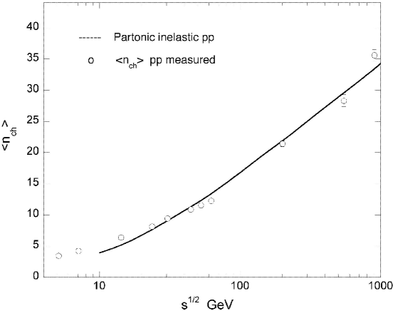
In the present approach each nucleon-nucleon collision has a hard scattering between two partons, leading to a system of two back to back $e^{+}e^{-}$-like jets with multiplicities as a function of center of mass (cms) energy and particle composition obtained from $e^{+}e^{-}$ data e-jets . The collision is taking up a certain fraction, x, of the energy of each of the incoming nucleons, picked from an “effective” structure function distribution. A very simple probability distribution function is found adequate, i.e. $dW/dx=2*(1-x)$ , such that on average one third of the nucleon incoming energy participates in the hard scattering. Since the two parton energies are independent, the cms for the two-jet system is not the overall cms, but different from event to event.The remaining forward going nucleon systems are considered excited systems, each of which fragments into one nucleon and one $e^{+}e^{-}$-like jet. Here it is assumed that on average half the energy is taken by the nucleon, i.e. a flat x-spectrum is used for the nucleon energy. Figure 2 shows how this model reproduces the mean charged multiplicity in pp collisions in the energy range from 10 to 1000 GeV.

In the jet fragmentation the multiplicity of each jet is taken from a negative binomial distribution with the value of $k$ varying (decreasing) as a function of $\sqrt{s}$ and the longitudinal x-distribution is subsequently determined by one-dimensional longitudinal phase space.

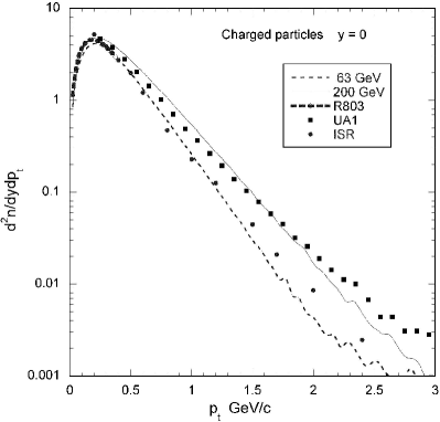
The transverse momentum is generated by a procedure taking into account the effect of gluon bremsstralung. This is done by giving the mean $p_{t}$ two components, one which is assumed constant $p_{t}^{out}$, and one increasing linearly with $\sqrt{s}$, $p_{t}^{in}$. This is in good qualitative agreement with $e^{+}e^{-}$ data, ref. inout . We find that adding (in quadrature) the transverse momenta from two independent $m_{t}$ distributions with inverse slopes of 0.090 GeV/c² for $p_{t}^{out}$ and 0.180+($\sqrt{s}$-20)*0.001 for $p_{t}^{in}$ gives a good agreement between the model and pp data, see Figure 4. Note that the effective parton-parton scattering angle distribution (see below) is also involved in generating the $p_{t}$ distributions shown. For forward nucleons a $p_{t}$ distribution with a negative inverse slope of 0.175 GeV/c is used.

Figure 2: Mean charged multiplicity in pp-collisions.

The next step is to obtain an effective parton-parton scattering angle distribution for the two-jet system. In this work a function from D. Perkins ( ref.Cambridge ) is used :

$$d\sigma/dcos\theta=const*(3+cos^{2}\theta)^{3}/(1-cos^{2}\theta)^{2},$$ (9)

An angle is found above a cut-off $p_{t,cut}$ following the above probability distribution and the corresponding jet $p_{t}$ is calculated. Finally this $p_{t}$ is reduced by the cut-off value : $p_{t,jet}=\sqrt{p_{t}^{2}-p_{t,cut}^{2}}$. The used value of the jet $p_{t}$-cutoff is $p_{t,cut}$= 0.3 GeV/c.

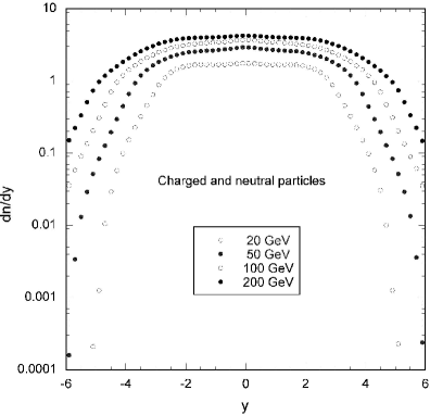
It should be noted that the parton-parton sub system production and fragmentation do not depend on the overall nucleon-nucleon (or AA) collision energy. Figures 3 and 4 show the rapidity and $p_{t}$ distributions obtained at different energies and illustrates in the $p_{t}$ case that qualitative agreement with the data is obtained.

Figure 3: Rapidity-distributions in pp collisions at cms energies of 20, 50, 100 and 200 GeV from the partonic model.

Figure 4: $p_{t}$ distributions from pp.The lower squares are from UA1 data at $\sqrt{s}=200$ GeV and the upper from from the ISR at $\sqrt{s}=50$ GeV. The dashed curves are partonic model results at 63 GeV (lower) and 200 GeV (upper).

III.3 The AA Model

The AA model is inspired by the work of Jackson and Boggild JandB and subsequent work JBblacklabel . Each AA collision, with specified impact parameter, involves a certain number of binary collisions, $N_{b}$, and of participants, $N_{p}$. The ratio of these numbers is the average number of collisions each struck nucleon experiences, $N_{c}=N_{b}/N_{p}$. If we now let a $train$ of $N_{c}$ nucleons from one nucleus collide with a similar $train$ from the other nucleus and do this $N_{p}/N_{c}$ times we get the right number of binary collisions. In each $train-train$ collision the procedure is the following using the above described parton inspired pp model:

a) The two $e^{+}e^{-}$ like jets escape the collision and fragment.

b) The forward wounded nucleon re-interacts with reduced energy.

c) At the end of the $train$ the wounded nucleon fragments as in the pp model.

In this way a collision of a $train$ of five against five nucleons will produce 10 wounded nucleons with successively reduced energy and 25 $e^{+}e^{-}$ like two-jet systems, in total leading to 50 (binary)+10(fragment) jets and ten nucleons.

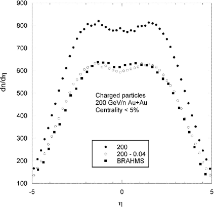
Figure 5 shows results of the model for central collisions of gold on gold, i.e. the pseudo-rapidity distributions before and after coalescence (see below) compared with BRAHMS data Brahms .

Figure 5: Pseudo-rapidity distributions for central Au+Au collisions at a cms energy of 200 GeV compared with data from Brahms Brahms . Full circles mark calculation at 200 GeV without pion coalescence (see text subsect. 3.4), while open circles denote the calculation including pion coalescence.

III.4 A modification of the Model

From Figure 5 it is clear that the AA model leads to charged particle multiplicities which are too high by 30-40%. This is not surprising since the model does not take shadowing shadow into account. Trying to model this by simply lowering the multiplicity does not work because energy conservation forces particles in the forward direction to take up the missing energy. This leads to a forward peaked rapidity distribution. To lower the multiplicity while maintaining energy-momentum conservation and the shape of the rapidity distribution a scheme of pion coalescing is adopted; the procedure used is the following :

a) The $Q^{2}_{inv}$ of all pion pairs is calculated, where
$Q^{2}_{inv}$ = $(E_{1}-E_{2})^{2}-(p_{x1}-p_{x2})^{2}-(p_{y1}-p_{y2})^{2}-(p_{z1}-p_{z2})^{2}$, and $E$ designates the total energy of the pion.
b) Pion pairs with $-Q^{2}_{inv}$ lower than a certain cutoff are coalesced.

It turns out that a cutoff at $-Q^{2}_{inv}=0.04^{2}$ GeV² leads to a reasonable reduction of the charged particle multiplicities and, at the same time, to a good agreement with observed rapidity distributions as demonstrated for BRAHMS in Figure 5. The assumption behind the above phenomenological procedure is that nearby pions are for some time after creation still overlapping and can act together. As further discussed below the price paid is a hardening of the pion $p_{t}$ distribution where the density is high.

The partonic model presented above in several respects resemble the HIJING-model of Wong and Gyulassy hiji .

IV Hadronic rescattering calculation

The rescattering model calculational method used is similar to that employed in previous calculations for lower CERN Super Proton Synchrotron (SPS) energies and RHIC studies Humanic:2002b . Rescattering is simulated with a semi-classical Monte Carlo calculation which assumes strong binary collisions between hadrons. The Monte Carlo calculation is carried out in three stages: 1) initialization and hadronization, 2) rescattering and freeze out, and 3) calculation of experimental observables. Relativistic kinematics is used throughout.

The hadronization model inputs momentum vectors from the thermal model or partonic jet model both described above and employs simple parameterizations to describe the initial space-time of the hadrons similar to that used by Herrmann and Bertsch Herrmann:1995a . The initial space-time of the hadrons for $b=0$ fm (i.e. zero impact parameter or central collisions) is parameterized as having cylindrical symmetry with respect to the beam axis. The transverse particle density dependence is assumed to be that of a projected uniform sphere of radius equal to the projectile radius, $R$ ($R={r_{0}}A^{1/3}$, where ${r_{0}}=1.12$ fm and $A$ is the atomic mass number of the projectile). The initial transverse coordinates of a given particle, i.e. $x_{had}$ and $y_{had}$, are thus determined according to this distribution. The longitudinal particle hadronization position ($z_{had}$) and time ($t_{had}$) are determined by the relativistic equations Bjorken:1983a ,

$$z_{had}=\tau_{had}\sinh{y_{i}};\hskip 8.53581ptt_{had}=\tau_{had}\cosh{y_{i}}$$ (10)

where $y_{i}$ is the initial particle rapidity and $\tau_{had}$ is the hadronization proper time. Thus the space-time hadronization model has one free parameter to extract from experiment: $\tau_{had}$. Although only pions, kaons, and nucleons are input from the thermal model as the initial particle types for the rescattering calculation, other types of hadrons can be produced during rescattering. In all, the hadrons included in the calculation are pions, kaons, nucleons, and lambdas ($\pi$, $K$, $N$, and $\Lambda$), and the $\rho$, $\omega$, $\eta$, ${\eta}^{*}$, $\phi$, $\Delta$, and $K^{*}$ resonances. For simplicity, the calculation is isospin averaged (e.g. no distinction is made among a $\pi^{+}$, $\pi^{0}$, and $\pi^{-}$).

The second stage in the calculation is rescattering which finishes with the freeze out and decay of all particles. Starting from the initial stage ($t=0$ fm/c), the positions of all particles are allowed to evolve in time in small time steps ($\Delta t=0.1$ fm/c) according to their initial momenta. At each time step each particle is checked to see a) if it has hadronized ($t>t_{had}$), b) if it decays, and c) if it is sufficiently close to another particle to scatter with it. Isospin-averaged s-wave and p-wave cross sections for meson scattering are obtained from Prakash et al. Prakash:1993a . The calculation is carried out to 100 fm/c, although most of the rescattering finishes by about 50 fm/c. The rescattering calculation is described in more detail elsewhere Humanic:2006a ; Humanic:1998a . The validity of the numerical methods used in the rescattering code have recently been studied and verifiedHumanic:2006b .

In the last stage of the calculation, the freeze-out and decay momenta and space-times are used to produce observables such as pion, kaon, and nucleon multiplicities and transverse momentum and rapidity distributions. The values of the initial pion, kaon, and nucleon multiplicities, temperature, and hadronization proper time are all constrained to give observables which agree with available measured hadronic observables. As a cross-check on this, the total energy from the calculation is determined and compared with the RHIC center of mass energy of $\sqrt{s}=200$ GeV to see that they are in reasonable agreement. Particle multiplicities were estimated from the charged hadron multiplicity measurements of the RHIC PHOBOS experiment Back:2000a . Calculations were carried out using isospin-summed events containing at freezeout for central collisions ($b=0$ fm) about 5000 pions, 500 kaons, and 650 nucleons ($\Lambda$’s were decayed). The hadronization model parameter $\tau_{had}$=1 fm/c was used. It is interesting to note that the same value of $\tau_{had}$ was required in a previous rescattering calculation to successfully describe results from SPS Pb+Pb collisions Humanic:1998a .

V Results from the thermal model with rescattering

V.1 $dn/dy$ with and without rescattering

This subsection demonstrates the changes in the rapidity density distributions caused by the rescattering. The rescattering routine was run event by event and 20 events made up the total final event pool, which was analyzed into $dn/dy$ and invariant cross section distributions. The thermal model sometimes produces particles with very large rapidities (e.g. $\mid y\mid\geq$10) in the forward and backward directions. These particles do not have a counterpart in a collision situation at any existing accelerator, so all particles with $\mid y\mid\geq$ 6.5 were disregarded in the rescattering calculation. $y=6.5$ is the beam rapidity at RHIC for the data used in the subsequent comparisons (subsect. 5.3). Such high rapidity particles constituted about 9% of the four-vectors generated by the thermal model and after their removal, the total energy of the remaining particles in a $T=200$ MeV event was close to the total energy in a $\sqrt{s}=200$ GeV Au+Au collision.

Figure 6: Rapidity distributions from the thermal model with $T=200$ MeV; open circles denote the results before rescattering and the black circles after. $N/10$ in the figure stands for nucleon multiplicity divided by 10.

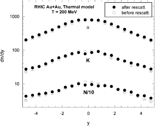
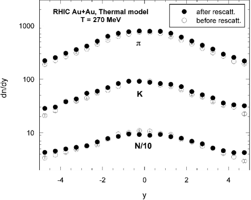
The resulting $dn/dy$ distributions at a temperature of $T=200$ MeV for pions, kaons and nucleons are shown in Figure 6, where open circles denote the distributions before rescattering and black circles after rescattering. Figure 7 shows results at $T=270$ MeV. In all cases the influence of the rescattering is finite and rather small. For nucleons the dn/dy with rescattering is lower by less than 5% at small $y$, than without rescattering, and higher by a similar amount at high rapidities. Kaons are changed less and in a similar way, and the pions are still less changed. Also the changes in going from 200 MeV to 270 MeV are quite small.

Figure 7: Rapidity distributions from the thermal model with $T=270$ MeV; open circles denote the results before rescattering and the black circles after. $N/10$ in the figure stands for nucleon multipicity divided by 10.

V.2 Invariant multiplicities with and without rescattering

The invariant multiplicities are analyzed as functions of either transverse momentum, $p_{t}$, or transverse mass, $m_{t}=\sqrt{p_{t}^{2}+m^{2}}$:

$$E\frac{d^{3}n}{dp^{3}}=\frac{d^{2}n}{2\pi m_{t}dm_{t}dy}=\frac{d^{2}n}{2\pi p_{t}dp_{t}dy},$$ (11)

where the multiplicity is denoted by $n$. In all cases shown the rapidity width in the model analysis is $\Delta y=1.0$, while the $m_{t}$ interval was 0.2 GeV.

For an isotropic Boltzmann source the shape of the invariant $m_{t}$-spectrum reflects the temperature $T$ as

$$\frac{1}{2\pi m_{t}}\frac{d^{2}n}{dm_{t}dy}=N_{Bol}m_{t}\cosh(y-y_{C})\exp{(-\frac{m_{t}}{T/\cosh(y-y_{C})})},$$ (12)

where $y_{C}$ is the rapidity of the source and $N_{Bol}$ the usual Boltzmann normalization (see also Eq. (2). The present thermal model represents the sum over many single particle sources, centered around three source centers, and will not show spectra following Eq. (12), nor the $1/\cosh(y-y_{C})$ dependence of the apparent temperature. None the less, the $m_{t}$-spectra are nearly exponential as in Eq. (12), and they exhibit an inverse slope that varies with rapidity in a way that also depends on particle mass, a feature that is different from the single spherical Boltzmann source, where the mass only enters explicitly in the normalization.

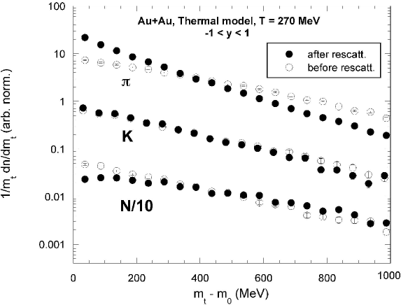
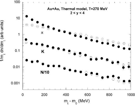
Figures 8 and 9 show the $m_{t}$-spectra before and after rescattering at $T=270$ MeV for rapidity zero and for rapidities near 3, respectively. The rescattering produces a steeper fall off with $m_{t}$ for pions at both rapidity zero and 3.35, the rescattering, so to speak, cools the pions. Kaons are influenced by the rescattering in a similar way, but to a smaller degree, while the nucleon spectrum becomes less steep in its fall off with $m_{t}$ at midrapidity, the nucleons get heated by the collisions with pions. At $y=3$ the nucleon spectrum is not changed by the rescattering. The inverse slopes are quantified in Table II, with the help of exponential fits to the spectra of Figures 8 and 9, where the fitting ranges correspond to the $m_{t}$ ranges in the figures for each spectrum. The inverse slopes change with rapidity in a distinct way for each particle type, reflecting the relative weighting of the contributions from the middle and forward-backward source-centers. The inverse slopes also increase markedly with mass of the particle, a feature normally taken to be indicative of flow, something that has not been introduced explicitly in the model.

Figure 8: Transverse mass spectra for $T=270$ MeV collected for rapidities around zero. The open circles mark results before rescattering, the black circles after rescattering. $N/10$ denotes nucleon multiplicity divided by 10.

Figure 9: Transverse mass spectra for $T=270$ MeV collected for rapidities around three. The open circles mark results before rescattering, the black circles after rescattering and $N/10$ denotes nucleon multiplicity divided by 10.

Table 2: Inverse slope parameters (MeV) from the thermal model for T=270 MeV.

particle	y	after	slope	error	before	slope	error
$\pi$	0		195	1		351	3
K			267	5		300	6
N			449	13		301	6
$\pi$	3		195	2		326	4
K			259	7		289	9
N			313	9		293	8

V.3 Comparison with experimental data

The rescattering, as discussed above, has little influence on the model predictions for $dn/dy$, just as the increase in temperature from 200 to 270 MeV has. Therefore the agreement with data is similar to what was shown in Figure 1. The figure shows protons and antiprotons separately and the comparison after rescattering should rather be with nucleons; a comparison of proton plus antiproton data, however does not change the quality of the agreement.

The model predictions for protons and antiprotons at $T=200$ MeV have $N_{\bar{p}0}/N_{p0}$=0.94 (see Table I), where a value of 1.0 would indicate a midrapidity source center with equal number of protons and antiprotons, i.e. a baryon chemical potential of zero. This follows because the F-functions in Eq. (3) are identical for $p$ and $\bar{p}$. A fit with an N-ratio of 1 could not be enforced with the present source-center geometry, as it would require negative forward and backward antiproton sources.

Figure 10: Comparison of transverse momentum spectra for $T=270$ MeV and data from BRAHMS at midrapidity. The data are denoted by open circles and are from references Peter 2003 and Djamel 2004 . The K-meson multiplicities have been divided by 10 and the proton data by 1000. The model results are for nucleons rather than protons.

Figure 11: Comparison of transverse momentum spectra for $T=270$ MeV and data from BRAHMS at rapidities about three. The data are denoted by open circles and are from references Peter 2003 and Djamel 2004 . The K-meson multiplicities have been divided by 10 and the proton data by 1000. The model results are for nucleons rather than protons.

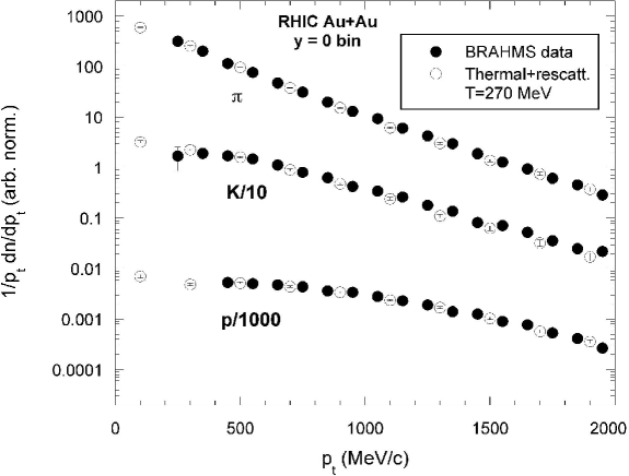
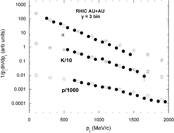
The comparison between data and model for the $p_{t}$-spectra is shown in Figures 10 and 11 at 270 Mev. For $y=0$ (Figure 10) the agreement between model and data is good and at $y=3$ (Figure 11) the agreement is reasonable. Thus the model can reproduce the data quite well at $T=270$ Mev at both rapidity intervals. It may be noted that the experimental $p_{t}$ spectra for protons and antiprotons exhibit nearly identical slopes Peter 2003 so the comparison of nucleon spectra from the model calculations to proton data is valid.

VI Results from the partonic model with rescattering

VI.1 Comparison of results with and without rescattering

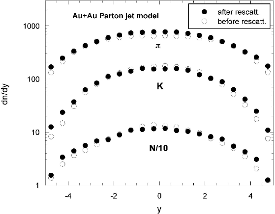
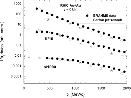
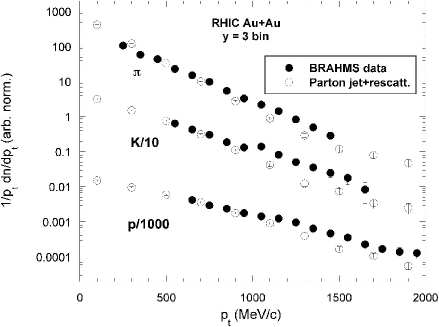
Figure 12 shows the $dn/dy$ distributions for $\pi$, $K$ and nucleons from the partonic model (open circles) and after rescattering (black circles). The data cover 20 events as for the thermal model results. In agreement with the thermal model results, the rescattering changes the distributions by very little, they are slightly broadened. The $m_{t}$ spectra however are markedly influenced; the rescattering makes the $\pi$ spectra steeper and flattens the $K$ and nucleon spectra, in particular at mid-rapidity. The effect for nucleons at mid-rapidity is somewhat stronger than for the thermal model, demonstrated by the inverse slopes obtained from exponential fits quoted in Table III for the partonic model and in Table II (above) for the thermal model. The changes are in the same directions as for the thermal model calculations.

Figure 12: Rapidity density $dn/dy$ as plotted versus center of mass rapidity. The results before rescattering are marked with open symbols, those after with black circles. The notation $N/10$ stands for nucleon multiplicity divided by 10.

Table 3: Inverse slope parameters (MeV) from the partonic jet model.

particle	y	after	slope	error	before	slope	error
$\pi$	0		165	1		299	2
K			230	3		168	2
N			358	8		167	2
$\pi$	3		143	1		196	1
K			166	3		141	3
N			201	4		150	3

The changes for nucleons caused by the rescattering are indeed quite dramatic, as is the cooling of the pions.

VI.2 Comparison to data

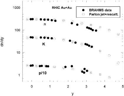
The $dn/dy$ distributions after rescattering are compared to the data for $\pi$, $K$ and nucleons in Figure 13, where the data are for protons rather than for nucleons. The agreement between model predictions and data are reasonable, but not as good as for the thermal case in Figure 1; it should be remarked, though, that in the thermal case there was a parameter adjustment for each particle species. The $p_{t}$ distributions are compared to data in Figures 14 and 15, where the agreement is very good both at midrapidity and near $y=3$. Inverse slopes vary with mass (see also Table III) in a way expected for flow, again without flow appearing explicitly in the calculations. In both cases, $dn/dy$ and transverse spectra, the data are shown for protons rather than nucleons ($p+\bar{p}$), but the conclusions drawn are not affected.

Figure 13: Rapidity densities versus center of mass rapidity. The data from referencesPeter 2003 and Djamel 2004 are plotted with black circles, while the results from the partonic model (after rescattering) are shown as open symbols.

Figure 14: Transverse momentum spectra at midrapidity, a comparison between data and model. The data are denoted by open circles and are from references Peter 2003 and Djamel 2004 . The K-meson multiplicities have been divided by 10 and the proton data by 1000. The model results are for nucleons rather than protons.

Figure 15: Transverse momentum spectra near $y=3$, a comparison between data and model. The data are denoted by open circles and are from references Peter 2003 and Djamel 2004 . The K-meson multiplicities have been divided by 10 and the proton data by 1000. The model results are for nucleons rather than protons.

VII Discussion

The two event generating models used here are very different and rather schematic. The thermal-like model has no dynamical features and therefore little predictive power, the fitting procedure described in Subsection 2.3 will have to be repeated at each incident energy, and the direct agreement with experiment without rescattering regarding the transverse spectra is rather poor. The partonic model is in principle a dynamic model with predictive power, however the pion coalescence mechanism is certainly ad hoc and may have to be adjusted at each incident energy. Also here the predicted transverse spectra agree rather poorly with experiment without rescattering. The main goal in this work has been to study the effects of hadronic rescattering on the hadrons produced by the two different models of the initial stage of the collision, and although the two models are very different, i.e. thermal-like hadrons vs. parton jets, after rescattering they both give similar hadronic rapidity, $m_{t}$, and $p_{t}$ distributions, which agree reasonably well with RHIC experiments. Although rescattering has only a weak effect on the rapidity distributions for either model, it is seen to strongly affect the $m_{t}$ (and $p_{t}$) distributions. For the thermal model with $T=270$ MeV, see Table II, the initial slope parameters are similar for the three particle species implying no initial radial flow from the model, whereas after rescattering the slope parameter increases significantly for increasing particle mass, and a radial flow effect like the experiments is seen. The slope parameters from the parton model also show radial flow and agree with experiments after rescattering, but as seen in Table III, before rescattering the slope parameters actually decrease significantly with increasing particle mass indicating a sort of “anti-radial-flow” effect. Thus even though the two models strongly disagree in the $m_{t}$ distributions they directly produce for the three particle species, rescattering effects are able to sufficiently wash out these differences such that after rescattering the particle distributions are now in essential agreement. We conclude from this that features seen in $m_{t}$ (and $p_{t}$) distributions before rescattering are mostly due to the overall temperature scale of the initial stage and rescattering effects are not very sensitive to the details of the initial stage model used. It is however remarkable that the rescattering changes the spectra in the same fashion as found in an earlier publication Humanic:1998a where a third event generator model was used: “cooling” of the pion spectra and “heating” of the nucleon spectra with the kaons in between.

Figure 16: Inverse slopes with rescattering for the thermal model plotted versus time. The inverse slopes were found from exponential fits to the $m_{t}$ spectra at the the various times. See also the text.

Figure 17: Inverse slopes with rescattering for the partonic model plotted versus time. Notation and definitions are as in the previous figure.

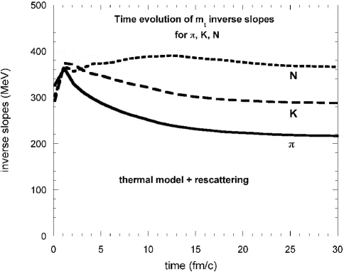
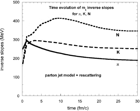
The two last figures, Figures 16 and 17, show the inverse slopes for $m_{t}$ spectra from the thermal-like and the partonic model both with rescattering, respectively, plotted versus time, $t$. The density of particles builds up as $t$ increases from zero until the volume increase with time overtakes the formation of new particles and the density starts to decrease, which happens at about $t=4$ fm/c. At large $t$ a steady state is reached for the inverse slopes and the pattern of increasing inverse slope with increasing particle mass, seen from Tables II and III has become evident. The changes at small times are very fast and the pushing of the faster pions on the other particles is clear while the pions themselves loose momentum. The first ten fm/c are very important for the development of the final slope pattern. The inverse slopes in the two figures do not agree quantitatively with the numbers in Tables II and III, at low $t$ because new particles enter fast as their formation times are reached, while in the tables the spectra are for all particles at freeze out, and moreover because rapidity ranges and $m_{t}$ ranges for the exponential fittings are different between tables and Figures 16 and 17. The conclusion is that to the extent the model approaches used here reflect in some reasonable way what happens in the real heavy ion collisions in the laboratory, one should evidently not draw strong conclusions from the hadronic $y$ and $m_{t}$ spectra neither regarding the presence of flow nor regarding the initial collision conditions.

It would be interesting to look at other hadronic observables such as elliptic flow and HBT interferometry using these two models to see if such observables can be used to discriminate between initial conditions.