Resumo

A produção de piões em colisões nucleão-nucleão, junto ao limiar, tem sido um desafio nas últimas décadas. A reacção $pp\rightarrow pp\pi^{0}$ em particular, é muito sensível a mecanismos de curto alcance porque a conservação do isospin suprime o termo de troca de piões que de outra forma seria dominante. Assim, tem sido muito difícil estabelecer a relativa importância dos vários processos de reacção.

Após rever o estado-da-arte da teoria, abordamos a validade da distorted-wave Born approximation (DWBA), através da sua ligação aos diagramas da teoria das perturbações ordenadas no tempo (TOPT). Analisamos igualmente as escolhas possíveis para a energia do pião trocado, inevitáveis no formalismo não-relativista subjacente a DWBA.

O operador de re-dispersão resultante de TOPT é comparado com o obtido pela abordagem mais simples de matriz-S, que tem sido usada eficazmente abaixo do limiar. A técnica de matriz-S, tendo reproduzido os resultados de TOPT para a re-dispersão em $pp\rightarrow pp\pi^{0}$ é aplicada à produção de piões neutros e carregados, descrevendo-se com sucesso as secções eficazes nestes diferentes canais. Os principais mecanismos de produção e ondas parciais correspondentes a momento angular mais elevado são incluídos. Finalmente, discutimos o efeito na secção eficaz das aproximações usuais para a energia do pião trocado.

PALAVRAS-CHAVE:
Produção de piões, prescrições de energia, matriz-S, DWBA, teoria das perturbações ordenadas no tempo, re-dispersão.

Abstract

Understanding pion production in nucleon-nucleon collisions near threshold has been a challenge for the last decades. In particular, the reaction $pp\rightarrow pp\pi^{0}$ is highly sensitive to short-range mechanisms, because isospin conservation suppresses the otherwise dominant pion exchange term. However, the relative importance of the various reaction processes has been very difficult to establish.

After reviewing the state-of-the-art of the theoretical approaches, we address the validity of the distorted-wave Born approximation (DWBA) through its link to the time-ordered perturbation theory (TOPT) diagrams. As the energy of the exchanged pion is not determined unambiguously within the non-relativistic formalism underlying DWBA, we analyse several options to determine which one is closer to TOPT.

The S-matrix technique, successfully used below threshold, is shown to reproduce the results of TOPT for the re-scattering mechanism in $\pi^{0}$ production. It is afterwards applied to full calculations of both charged and neutral pion production reactions, the cross sections of which are described successfully. The main production mechanisms and partial waves corresponding to high angular momentum are included in the calculations. Finally we discuss the effect on the cross section of the frequent prescriptions for the energy of the exchanged pion.

KEYWORDS:
Pion production, energy-prescriptions, S-matrix, DWBA, time-ordered perturbation theory, re-scattering.

Preface

The study of pion production processes close to threshold was originally initiated to explore the application of fundamental symmetries to near-threshold phenomena. These investigations on meson production reactions from hadron-hadron scattering began in the fifties, when high energy beams of protons became available. A strong interdependence between developments in accelerator physics, detector performance and theoretical understanding led to an unique vivid field of physics.

Triggered by the unprecedented high precision data for proton-proton induced reactions (in new cooler rings), the interest on pion production studies was revitalised in the last decade. The (large) deviations from the predictions of one-meson exchange models controlled by the available phase-space, are indications of new and exciting physics.

The reaction $NN\rightarrow NN\pi$ is the basic inelastic process related to the nucleon-nucleon ($NN$) interaction. It sheds light on the $NN$ and $\pi N$ interactions and is key to understanding pion production in more complex systems. Close to the threshold the process is simpler because it is characterised only by a small number of combinations of initial and exit channels. Moreover, at these reduced energies, meson production occurs with large momentum transfers, making it a powerful tool to study short range phenomena.

Pion production occurs when the mutual interaction between the two nucleons causes a real pion to be emitted. The other contribution comes from a virtual pion being produced by one nucleon and knocked on to its mass shell by an interaction with the second nucleon. This is the so-called re-scattering diagram, which is found to be highly sensitive to the details of the calculations, namely the treatment of the exchanged pion energy.

This pion re-scattering mechanism is suppressed in $pp\rightarrow pp\pi^{0}$ due to isospin conservation. The transition amplitude then results from a delicate interference between various additional contributions of shorter range. A treatment of these mechanisms consistent with the $NN$ interactions employed in the distortion of the initial and final state is essential to clarify this large model dependence. In this work, a consistent description of not only neutral, but also charged pion production, is shown to be possible.

In this thesis we will address the problem of charged and neutral pion production in nucleon-nucleon collisions. The main steps of this investigations are:

1. Starting with relativistic field theory, time-ordered perturbation theory (TOPT) is used to justify the distorted-wave Born approximation (DWBA) approach for pion production;

2. Using the DWBA amplitude fixed by TOPT as a reference result, the effect of the traditional prescriptions for the energy of the exchanged pion in the re-scattering operator is analysed;

3. Defining a single effective production operator within the S-matrix technique, its relation to the DWBA amplitude yielded by TOPT is established;

4. Employing the S-matrix approach, charged and neutral pion production reactions are described consistently.

This work is based on the following publications:

• V. Malafaia and M. T. Peña, Pion re-scattering in $\pi^{0}$ production, Phys. Rev. C 69 (2004) 024001 [nucl-th/0312017].

• V. Malafaia, J. Adam and M. T. Peña, Pion re-scattering operator in the S-matrix approach, Phys. Rev. C 71 (2005) 034002 [nucl-th/0411049].

• V. Malafaia, M. T. Peña, Ch. Elster and J. Adam, Charged and neutral pion production in the S-matrix approach, [nucl-th/0511038], submitted to Phys. Lett. B.

• V. Malafaia, M. T. Peña, Ch. Elster and J. Adam, Neutral and charged pion production with realistic $NN$ interactions, to submit to Phys. Rev. C.

Chapter 1 introduces the physics accessible through the study of the meson production reactions. It focuses on the specific aspects of hadronic meson production reactions close to threshold, namely the rapidly varying phase-space, the (high) initial and (low) final relative momenta, and the general energy dependence of the production operator.

Chapter 2 is a historical review of the main theoretical approaches to pion production developed so far. The first part is dedicated to the distorted-wave Born approximation (DWBA), the frequently used approach in all the calculations near the threshold energy, in which the nucleon-nucleon interaction is treated non-perturbatively, whereas the transition amplitude $NN\rightarrow NN\pi$ is treated perturbatively. The second part focuses on the coupled-channel phenomenological approaches and the third part aims to present the actual status of chiral perturbation theory ($\chi$PT) calculations.

DWBA calculations apply a three-dimensional formulation for the initial- and final-$NN$ distortion, which is not obtained from the Feynman diagrams. As a consequence, in calculations performed so far within the DWBA approximation, the energy of the exchanged pion has been treated approximately and under different prescriptions. A clarification of these formal issues is thus needed before one can draw conclusions about the physics of the pion production processes. The re-scattering mechanism, being highly sensitive to these energy prescriptions, is the ideal starting point for this clarification.

Chapter 3 aims to obtain a three-dimensional formulation from the general Feynman diagrams. This chapter discusses the validity of the DWBA approach by linking it to the time-ordered perturbation theory (TOPT) diagrams which result from the decomposition of the corresponding Feynman diagram. Since in the time-ordered diagrams energy is not conserved at individual vertices, each of the re-scattering diagrams for the initial- and final-state distortion defines a different off-energy shell extension of the pion re-scattering amplitude. This imposes the evaluation of the matrix elements between quantum mechanical wave functions, of two different operators. Henceforth, in Chapter 4 we are lead to an alternative approach to the TOPT formalism (the S-matrix approach), which in contrast to it avoids this problem.

The S-matrix approach provides a consistent theoretical framework for the two diagrams, as well as for the $NN$ distortion. Besides, from the practical point of view, it simplifies tremendously the numerical effort demanded in TOPT by the presence of logarithmic singularities in the pion propagator for ISI. The S-matrix construction has already been successfully used below pion production threshold and in particular for $NN$ interactions and electroweak meson exchange currents. In Chapter 4 also, the effective DWBA amplitude obtained in Chapter 3 is employed to re-examine the nature and extent of the uncertainty resulting from the approximations made in the evaluation of the effective operators.

In Chapter 5, the S-matrix technique, shown in Chapter 4 to reproduce the results of time-ordered perturbation theory for the re-scattering mechanism in $\pi^{0}$ production, is applied to charged and neutral pion production reactions. The major production mechanisms, namely the contributions from the direct-production, re-scattering, Z-diagrams and $\Delta$-isobar excitation are considered. Higher angular momentum partial waves, which are not included in traditional calculations, are also considered. The last part is dedicated to the effect on the cross section of the usual prescriptions for the energy of the exchanged pion. For all the charge channels, the S-matrix approach for the description of the pion production operators reproduces well the DWBA result coming from TOPT. Importantly, the effect of some approximations usually employed is also assessed. The $\pi^{+}$ reaction is seen to be especially sensitive to those. Previous failures in its description are overcome and clarified.

Finally, in Chapter 6 we outline and summarise the most relevant aspects discussed in this thesis, and mention the future prospects of pion production in nucleon-nucleon collisions.

Chapter 1 Meson production close to threshold

Abstract: Meson production reactions in nucleonic collisions near threshold are a powerful tool to investigate short-range phenomena. Pion production reactions play a very special role, since they yield the lowest hadronic inelasticity for the nucleon-nucleon interaction and thus they are an important test of the phenomenology of the nucleon-nucleon interaction at intermediate energies.

1.1 What physics can we learn from meson production reactions?

Quantum Chromodynamics (QCD), the fundamental theory for strong interactions, unfolds an impressive predictive power mainly at high energies. However, at low energies the perturbative expansion no longer converges.

Although a large amount of data on hadronic structure and dynamics is available from measurements with electromagnetic probes (for instance, from MAMI at Mainz, ELSA at Bonn and JLAB at Newport News), there is still much to be learned about the physics with hadronic probes at intermediate energies, comprising the investigation of production, decay and interaction of hadrons. In particular, meson production reactions (close to threshold) in nucleon-nucleon, nucleon-nucleus and nucleus-nucleus collisions constitute a very important class of experiments in this field.

With the advent of strong focusing synchrotrons having high-quality beams (for instance, the IUCF Cooler in Bloomington, CELSIUS in Upsala and COSY in Jülich), a new class of experiments could be performed in the last decade, differing from the previous ones with respect to the unprecedented quality of the data (polarised as well as unpolarised) for several $NN\rightarrow NNx$ reaction channels (a recent review on the experimental and theoretical aspects of meson production can be found in Refs. [1, 2] and in Ref. [3], respectively).

The study of meson production close to threshold has several attractive key features, in particular concerning,

• Large momentum transfer in the entrance channels
  Meson production near threshold occurs at large momentum transfers and therefore is a powerful tool to study short range phenomena in the entrance channel;

• Simplicity of the entrance and exit channels
  The analysis of the reaction data is straightforward allowing one to study the underlying reaction mechanisms;

• Small phase-space
  Only a very limited part of the phase-space is available for the reaction products and hence, only a few partial waves contribute to the observables, especially very near the threshold.

Although a small number of partial waves is clearly an advantage for calculations, on the other hand, as a result of the small phase-space, the cross sections are also small. There is a delicate interplay between the several possible reaction mechanisms and thus it is essential that all the technical aspects are under control for a meaningful interpretation of the data.

The large momentum transfer can also look like an disadvantage since it is difficult to reliably construct the production operator. However, in the regime of small invariant masses, the production operator is largely independent of the relative energy of a particular particle pair in the final state. Consequently, dispersion relations can be used to extract low-energy scattering parameters of the final state interaction and at the same time, to estimate the error in a model independent way.

In the overall, meson production reactions in nucleonic collisions have a huge potential to give insight into the strong interaction physics at intermediate energies, namely concerning the following aspects:

• Final state interactions
  Scattering of unstable particles off nucleons is experimentally very problematic since it is difficult to prepare intense beams of these particles with the required accuracy. Production reactions where such particles emerge in the final state are an attractive alternative.

• Baryon resonances in a nuclear environment
  The systems studied in nucleon-nucleon and nucleon-nucleus collisions allow to investigate particular resonances in the presence of other baryons and excited by various exchanged particles. One example is the $N^{*}\left(1535\right)$, which is clearly visible as a bump in any $\eta$ production cross section[3].

• Charge symmetry breaking
  The existence of available several possible initial isospin states (for instance $pp$, $pn$ and $dd$), with different possible spin states, allows experiments which enable the study of isospin symmetry breaking.

• Effective field theory in large momentum transfer reactions
  The investigation of hadronic processes at low and intermediate momenta are essential to test the convergence of the low-energy expansion of chiral perturbation theory ($\chi$PT).

• Three-nucleon forces
  The information on the short-range mechanisms that can be deduced from pion production in nucleon-nucleon ($NN$) collisions is relevant for constraining the three-nucleon forces[4].

This work will focus on pion production reactions in nucleon-nucleon collisions. It is the lowest hadronic inelasticity for the nucleon-nucleon interaction and thus an important test of the understanding of the phenomenology of the $NN$ interaction. Secondly, as pions are the Goldstone bosons of chiral symmetry, it is possible to study pion production also using $\chi$PT. This provides the opportunity to improve the phenomenological approaches via matching to the chiral expansion, as well as to constrain the chiral contact terms via resonance saturation. As mentioned before, a large number of (un)polarised data is available to be used as constraints. Moreover, meson-exchange models of the nucleon-nucleon interaction above the pion threshold rely on detailed information about the strongly coupled inelastic channels which must be treated together with the elastic interaction. Also, information on pion production in the $NN$ system is required in models of pion production or absorption in nuclei.

1.2 Specific aspects of hadronic meson production close to threshold

1.2.1 Rapidly varying phase-space

Threshold production reactions are characterised by excess energies which are small compared to the produced masses. In the near threshold regime the available phase-space changes very quickly (although remaining small). Therefore, to compare different reactions, one needs an appropriate measure of the energy relative to threshold. For pion production, the traditionally used variable is the maximum pion momentum $\eta$ (in units of the pion mass). For all heavier mesons, the so-called excess energy $Q$, defined as

$$Q=\sqrt{s}-\sqrt{s^{threshold}},$$ (1.1)

is used instead. In Appendix A, a compilation of useful kinematic relations is presented, and the importance of relativistic kinematics for the near threshold reactions is stressed.

If $Q$ gives the available energy for the final state, the interpretation of $\eta$ is somewhat more involved. In a non-relativistic, semiclassical picture, the maximum angular momentum allowed can be estimated via

$$l_{max}\simeq Rq^{\prime},$$ (1.2)

where $R$ is a measure of the force range and $q^{\prime}$ is the typical momentum of the corresponding particle. Identifying $R$ with the Compton wavelength of the meson of mass $m_{x}$, $\eta$ can be interpreted as the maximum angular momentum allowed[5]:

$$l_{max}\simeq\frac{q^{\prime}}{m_{x}}\simeq\eta\hskip 28.45274pt(\mathrm{with}\hskip 5.69046pt\hbar=c=1).$$ (1.3)

To compare the cross sections for reactions with different final states in order to extract information about the reaction mechanisms, one has to choose carefully the variable that is used to represent the energy. Indeed, as it is shown in Fig. 1.1, the total cross sections for $pp\rightarrow pp\pi^{0}$, $pp\rightarrow pp\eta$ and $pp\rightarrow pp\eta^{\prime}$ are different when compared at equal $\eta$ (panel (b)) or at equal $Q$ (panel (a)).

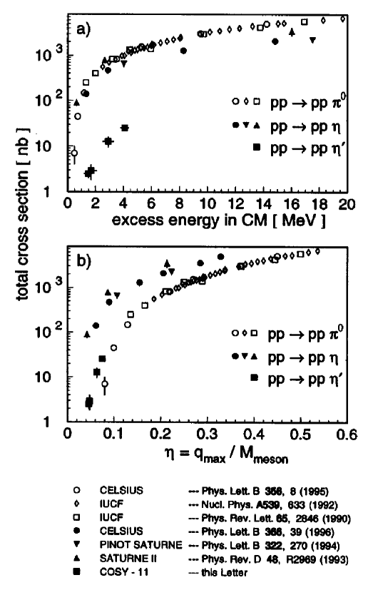
Figure 1.1: Total cross sections for the reactions $pp\rightarrow pp\pi^{0}$, $pp\rightarrow pp\eta$ and $pp\rightarrow pp\eta^{\prime}$ as a function of a)the excess energy $Q$ and b)the maximum pion momentum $\eta$ in units of the mass of the produced meson. Figure taken from Ref. [6].

When the dominant final state interaction is the $pp$ interaction, which is the case for those reactions, it appears thus to be more appropriate to compare the cross sections at equal $Q$, since then at any given energy, the impact of the final state interaction is equal for all the reactions. This is not the case for equal values of $\eta$, as $\eta$ depends on the mass of the produced meson.

1.2.2 Initial and final relative momenta

Meson production in nucleon-nucleon collisions requires that the kinetic energy of the initial particles is sufficiently high to put the outgoing meson on its mass shell. In other words, the relative momentum of the initial nucleons must exceed the threshold value,

$$p_{initial}^{th.}=\sqrt{m_{x}M+\frac{m_{x}^{2}}{4}},$$ (1.4)

where $M$ is the nucleon mass and $m_{x}$ is the mass of the produced meson. For a close-to-threshold regime, the particles in the final state have small momenta and thus $p_{initial}^{th.}$ also sets the scale for the typical momentum transfer. In a non-relativistic picture, this large momentum transfer translates into a small reaction volume, characterised by a size parameter,

$$R\sim\frac{1}{p_{initial}^{th.}}\simeq 0.5\mathrm{fm}\hskip 14.22636pt\text{for pion production}.$$ (1.5)

The two nucleons in the initial state have thus to approach each other very closely before the production of a meson can happen. For this reason it is important to understand not only the elastic but also the inelastic $NN$ interaction to obtain quantitative predictions.

1.2.3 Remarks on the production operator and nucleonic distortions

In the near threshold regime, all the particles in the final state have low relative momenta and thus can potentially undergo strong final state interactions (FSI) that can induce strong energy dependencies. On the other hand, close to the threshold, the initial energy is significantly larger than the excess energy $Q$, and consequently the initial state interaction (ISI) should at most mildly influence the energy dependence. The dependence of the production operator on the excess energy should also be weak, since it is controlled by the typical momentum transfer, which is significantly larger than the typical outgoing momenta. Fig. 1.2 illustrates the energy dependence of the production operator both FSI and ISI cases.

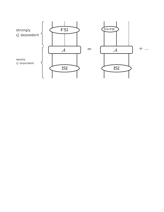
Figure 1.2: Sketch of the excess energy $Q$-dependence of the meson production reaction. $\mathcal{A}$ is the production operator. The left diagram shows the complexity possible, with interaction between the three final particles, whereas the right diagram shows the first and potentially dominant term (with FSI only for the two final nucleons).

The large momentum transfer characteristic of meson production reactions at threshold leads to a large momentum mismatch for any one-body operator that might contribute to the production reaction.

1.3 Theoretical considerations on $NN\rightarrow NNx$ reactions

Most of the theoretical models for the reactions $NN\rightarrow NNx$ can be grouped in two distinct classes:

• Distorted wave Born approximation (DWBA)
  A production operator is constructed within some perturbative scheme approximation and then is convoluted with the nucleon wave functions.

• (Truly) Non-perturbative approaches
  Integral equations are solved for the full $\left(NN,NNx\right)$ coupled-channel problem, describing multiple re-scattering and preserving three-body unitarity.

The great majority of theoretical studies of pion production in nucleon-nucleon collisions in the threshold region have been done within the DWBA formalism[9]. This approach is motivated by the fact that close to pion production threshold, where the kinetic energy of the particles in the final state is practically zero, the forces between the nucleons are much stronger than the interaction between the pion and the nucleon. Consequently, only the interaction between the nucleons is taken into account up to all orders, for instance, by employing wave functions that are solutions of a scattering (Lippmann-Schwinger) equation, whereas the pion production process is treated perturbatively and the pion is assumed to propagate freely after its production. Typically, the diagrams that contribute are of the type of those of Fig. 1.3.

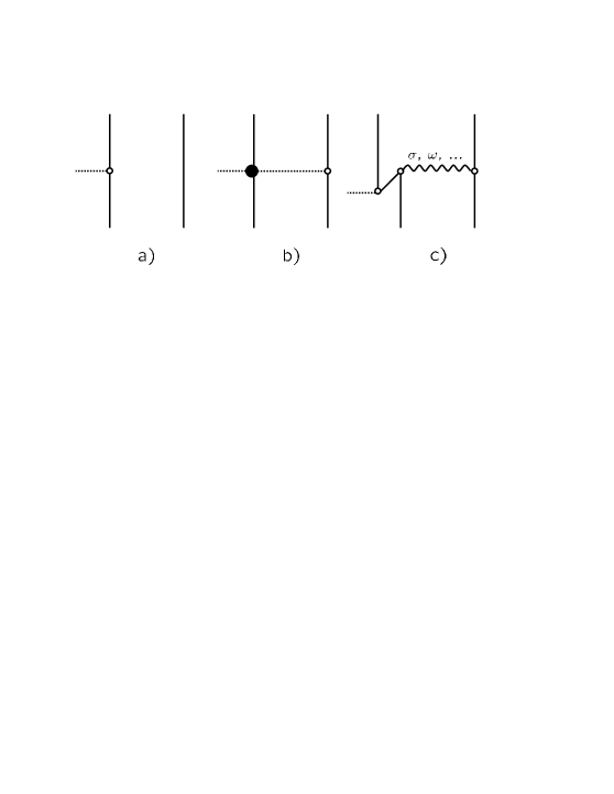
Figure 1.3: Contributions to the production operator in pion production in $NN$ collisions which in the DWBA formalism are convoluted with $NN$ wave functions: a) direct-production, b) re-scattering and c) short-range contributions. The solid and dotted lines represent the nucleons and pions, respectively.

On the other hand, all calculations performed so far for pion production within the full $\left(NN,NNx\right)$ coupled-channel approach were within the framework of time-ordered perturbation theory[10] (TOPT), or its extension to the $N\Delta$ sector done by the Helsinki[11, 12, 13], Argonne[14, 15, 16, 17] and Hannover[18, 19, 20] groups, which have a reasonable predictive power at higher energies but cannot describe the physics very near threshold, as discussed in Sec. 2.2.1.

1.4 The cross section

In Fig. 1.4, there is an overview of the total cross sections in $pp$ interactions below $4\mathrm{GeV}$ beam momentum.

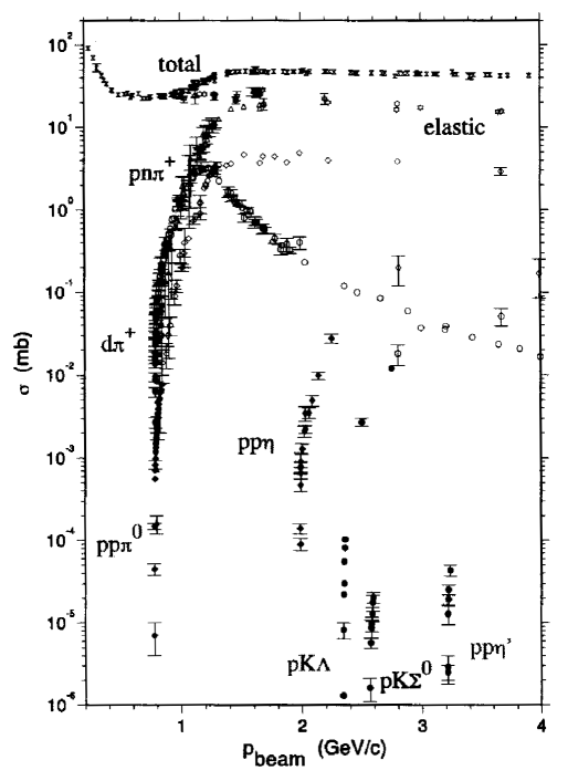
Figure 1.4: Cross sections for $pp$ interactions as a function of the beam momentum. Figure taken from Ref. [2].

In Table 1.1 we list the threshold momenta $p^{thr.}$ and threshold laboratory energies $T_{lab}^{thr.}$, for the $NN\rightarrow NN\pi$ reactions considered in this work. The right column is a compilation of references with the experimental determination of $\sigma_{tot}$.

The first threshold which opens with increasing beam energy is $\pi^{0}$ production followed very soon after by $\pi^{\pm}$ production (see Table 1.1). Pion production exhausts all inelasticity in this momentum range (see Fig. 1.4) and therefore is fundamental to understand the nucleon-nucleon interaction.

reaction	$p^{\text{thr.}}\left[\mathrm{MeV}\right]$	$T_{lab}^{\text{thr.}}\left[\mathrm{MeV}\right]$	$\sigma_{tot}$
$pp\rightarrow pp\pi^{0}$	$724.4$	$279.7$	[21, 22, 23, 24, 25, 26]
$pp\rightarrow pn\pi^{+}$	$737.3$	$289.5$	[27, 28, 29, 30]
$pn\rightarrow pp\pi^{-}$	$737.3$	$289.5$	[31, 32, 33]

Table 1.1: Threshold momenta and threshold laboratory energies for pion production reactions in the $NN$ collisions considered in this work. The right column refers to the experimental determination of the corresponding cross sections.

Chapter 2 State of the art of theoretical models for pion production

Abstract: The significant experimental progress in the last decade resulted in high-quality data on pion production near threshold. For neutral pion production these new and accurate data posed a theoretical challenge since they were largely under-predicted by the existent calculations. This Chapter is a historical review of the main theoretical approaches developed.

2.1 DWBA in the Meson exchange approach

2.1.1 Problems of the earlier calculations

The work of Koltun and Reitan

Pioneering work on pion production was done in the 1960s by Woodruf[9] and by Koltun and Reitan[34]. All later investigations of meson production, including the very recent efforts to analyse the high-precision data from the new generation of accelerators, have followed basically the same approach, if one excludes the Hannover model[18, 19, 20] for coupled $NN$, $N\Delta$-$NN\pi$ channels.

These works focused on the reactions $pp\rightarrow pp\pi^{0}$ and $pp\rightarrow d\pi^{+}$. The processes considered were direct production by either nucleon (diagram (a) of Fig. 2.1), the so-called impulse approximation, and production from pion-nucleon scattering (diagram (b)), the so-called re-scattering term.

Figure 2.1: The main mechanisms considered in the works on pion production: a) direct production, b) re-scattering, c) pion re-scattering via a $\Delta$ and d) short-range contributions. The solid and dashed lines represent the nucleon and pion fields, respectively. Heavy mesons ($\sigma$, $\omega$,…) are represented by the wavy line.

The $\pi N\rightarrow\pi N$ transition amplitudes were parameterised in terms of scattering lengths, through the Hamiltonian $\mathcal{H}=\mathcal{H}_{1}+\mathcal{H}_{2}$, with

$$\mathcal{H}_{1} = i\frac{f_{\pi NN}}{m_{\pi}}\vec{\sigma}\cdot\left[\vec{\nabla}_{\pi}\boldsymbol{\tau}\cdot\boldsymbol{\pi}+\frac{1}{2M}\left(\vec{p}\boldsymbol{\tau}\cdot\boldsymbol{\dot{\pi}}+\boldsymbol{\tau}\cdot\boldsymbol{\dot{\pi}}\vec{p}\right)\right]$$ (2.1)

$$\mathcal{H}_{2} = 4\pi\frac{\lambda_{1}}{m_{\pi}}\boldsymbol{\pi}\cdot\boldsymbol{\pi}+4\pi\frac{\lambda_{2}}{m_{\pi}^{2}}\boldsymbol{\tau}\cdot\boldsymbol{\pi}\times\boldsymbol{\dot{\pi}}$$ (2.2)

where $\vec{\sigma}$ and $\boldsymbol{\tau}$ are the usual nucleon spin and isospin operators, and $\vec{p}$ is the nucleon momentum operator. The pion(nucleon) mass is $m_{\pi}\left(M\right)$ and the pion field is $\boldsymbol{\pi}$. The $\pi NN$ pseudovector coupling constant is $f_{\pi NN}$.

$\mathcal{H}_{1}$ is obtained from a non relativistic reduction of the pseudovector $NN\pi$ vertex and gives diagram (a) in Fig. 2.1. The first term of Eq. (2.1) represents $p$-wave $\pi N$ coupling, while the second term (“galilean” term) accounts for the nucleon recoil effect[36]. For $s$-wave pion production, only the second term contributes. Since this second term is smaller than the first term by a factor of $\sim\frac{m_{\pi}}{M}$, the contribution of the Born term to $s$-wave pion production is intrinsically suppressed, and as a consequence the process becomes sensitive to two-body contributions, Fig. 2.1(b) and (d).

$\mathcal{H}_{2}$ is a phenomenological effective Hamiltonian describing pion re-scattering. The isoscalar and isovector parts of the $\pi N$ s-wave scattering amplitude, $\lambda_{1}$ and $\lambda_{2}$, were obtained from the $s$-wave phase shifts $\delta_{1}$ and $\delta_{3}$ for the pion-nucleon scattering, through the Born-approximation relations[34],

$$\lambda_{1}=-\frac{1}{6\eta}\left(\delta_{1}+2\delta_{3}\right)=0.005\hskip 71.13188pt\lambda_{2}=-\frac{1}{6\eta}\left(\delta_{1}-\delta_{3}\right)=0.045,$$ (2.3)

where $\eta$ is the maximum pion momentum (in units of $m_{\pi}$). Although $\lambda_{2}\gg\lambda_{1}$, the isospin structure of the $\lambda_{2}$ term is such that it cannot contribute to $\pi^{0}$ production.

We note that without initial- or final-state distortions, the diagram (a) of Fig. 2.1 vanishes because of four-momentum conservation. The calculations of Ref. [34] were performed using the Hamada-Johnston phenomenological potential for the $NN$ distortion, and neglecting the Coulomb interaction between the two protons. The calculated cross section for $pp\rightarrow pp\pi^{0}$ of $17\eta^{2}\mu b$ was found to be consistent with the measured cross section near threshold, which was, however, not well determined[37] by that time.

The role of final-state and Coulomb interactions

When the first high precision data[21] on the reaction $pp\rightarrow pp\pi^{0}$ appeared, they contradicted the predicted $\eta^{2}$ dependence near threshold. According to the work of Refs. [23, 38] the energy dependence of the $s$-wave cross section followed from the phase space and a simple treatment of the final-state interaction[39, 40] between the two (charged) protons. This was found sufficient to reproduce the shape of the measured cross section up to $\eta\simeq 0.5$ (see Fig. 2.2), where higher partial waves start to contribute[23]. Also, the inclusion of the Coulomb interaction was found to be essential to describe the energy dependence of the total cross section in particular for energies close to threshold. The validity of the effective-range approximation employed in Ref. [34] for the energy dependence of the final state turned out to be limited to energies rather close to threshold ($\eta\leq 0.4$).

However, the theory failed in describing quantitatively the cross section for $pp\rightarrow pp\pi^{0}$ by a factor of $5$, which was in contrast to the reaction $pp\rightarrow pn\pi^{+}$, where the discrepancy was less than a factor of $2$, as reported in Ref. [27].

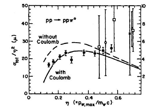
Figure 2.2: Energy dependence of the total cross section for the reaction $pp\rightarrow pp\pi^{0}$. The solid dots are data from Ref. [21]. The squares, cross and diamonds are older data. The solid curve is the full calculation and the dashed line shows the effect of omitting the Coulomb interaction. The data are to be evaluated using the scale on the left, while the theory used the scale on the right. Note that the calculations underestimate the data by a factor of $\sim 5$. Figure taken from Ref. [38].

Ref. [38] suggested that the problem arose from the use of an over-simplified pion nucleon interaction, namely in considering the exchanged pion to be on-shell. The on-shell $s$-wave pion nucleon interaction is constrained to be small by the requirements of chiral symmetry but, for the production reaction to proceed, either the re-scattered pion or a nucleon must be off-shell. This means that the $\pi N$ amplitude relevant for pion production must be larger than the theoretical one for on-shell particles, whose investigation was to be subsequently pursued.

The inclusion of the $\Delta$

The work of Ref. [41] considered the $p$-wave re-scattering through a $\Delta\left(1232\right)$ resonance (diagram c) of Fig. 2.1) by introducing finite-range $N\Delta$ coupled-channel admixtures to the nucleonic wave functions. The transition potential $NN\rightarrow N\Delta$ included both $\pi$ and $\rho$ exchanges. The pion production vertex was taken from Eq. (2.2) and including the relativistic effects arising from the use of the pion total energy $E_{\pi}$ instead of the pion mass (static approximation). The isoscalar and isovector parameters $\lambda_{1}$ and $\lambda_{2}$ of the phenomenological hamiltonian of Eq. (2.2) were allowed an energy dependence through the momentum of the pion. The results are shown in Fig. 2.3.

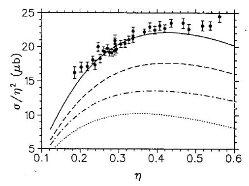
Figure 2.3: Cross section for $pp\rightarrow pp\pi^{0}$. The solid line is the full calculation. The dotted line is the direct production due only to second term of Eq. (2.1) and going beyond the static approximation, the dash-dotted line includes also re-scattering through the $\Delta$. The dashed line is the full purely nucleonic production. All the calculations were multiplied by a common arbitrary factor of $3.6$. The data points are from Ref. [21]. Figure taken from Ref. [41].

The small difference between the theoretical models was attributed to the different value used for the $\pi N$ coupling constant and to the relativistic kinematics. The inclusion of the non-galilean term and the $s$-wave scattering gave an enhancement of over $60\%$ (dashed curve). Another $25\%$ enhancement arose from the inclusion of the re-scattering through the $\Delta$. However, the cross section was still missed by almost a factor of $\sim 4$.

Charged pion production

The first calculations on $\pi^{+}$ production where those of Schillaci, Silbar and Young[42]. General isospin and phase space arguments[5, 40] were employed to predict the spin, isospin and energy dependence of the total cross section, including all partial waves for the $NN$ amplitudes, but accounting only for $s$-wave pion-nucleon states. It fails if contributions from the $\Delta$ resonance are significant.

The second prediction was made by Lee and Matsuyama[16] with a coupled channel formalism that focused on the effects of the $\Delta$ intermediate state. In Ref. [16, 17], the $\Delta$ process is handled rigorously while the non resonant pion production process is introduced as a perturbation. The estimated $\Delta$ contribution was roughly $15\%$ of the total cross section. Both calculations were not able to describe the experimental data for $pp\rightarrow pn\pi^{+}$ as it is shown in Fig. 2.4 (solid and dotted lines, respectively).

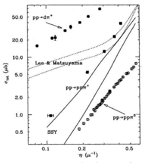
Figure 2.4: Comparison of measured total $pp\rightarrow pn\pi^{+}$ cross section with the theoretical predictions of Refs. [17, 42]. The solid lines are the calculations of Schillacci, Silbar and Young[42]. The dotted lines are the calculations of Lee and Matsyuama[17]. Figure taken from Ref. [27].

Calculations based on a relativistically covariant one-boson exchange model[43], also suggested that the contribution of a $\Delta$-isobar is not important at energies below $350\mathrm{MeV}$ (due to the fact that at lower energies pions are predominantly produced in a $\pi N$ relative $s$-state and thus the possibility of forming a $\Delta$-isobar is greatly reduced), but dominate at higher beam energies. The cross sections for $pp\rightarrow pn\pi^{+}$ near threshold were under-predicted a factor of $2$-$4$.

The work of Ref. [44] applied the Watson theorem[39] to the final state interaction of Ref. [43]. The calculated cross sections were within $25\%$ of the $pp\rightarrow pn\pi^{+}$ data[28], but were also under-predicted near threshold.

Also, in the work of Ref. [46], the isoscalar heavy meson exchange found to dominate in $pp\rightarrow pp\pi^{0}$ was however shown to be less significant in $pp\rightarrow pn\pi^{+}$, where the re-scattering diagram was the most important one. Further theoretical studies on these issues were then clearly needed to clarify the role of the different production mechanisms.

2.1.2 The first quantitative understandings

The first quantitative understanding of the $pp\rightarrow pp\pi^{0}$ data was reported by Lee and Riska[47] and later confirmed by Horowitz et al.[48], where it was demonstrated that short range mechanisms (diagram (d) of Fig. 2.1) can give a sizeable contribution. In these works, the difficulty in describing the cross section for $pp\rightarrow pp\pi^{0}$ was overcame by considering the pair terms, positive and negative energy components of the nucleon spinors, connected to the isoscalar part of the $NN$ interaction.

The importance of short-range mechanisms

In the work of Ref. [47], the short range two-nucleon mechanisms that are implied by the nucleon-nucleon interaction were taken into account by describing the pion-nucleus interaction by the extension of Weinberg’s effective pion-nucleon interaction to nuclei:

$$\mathcal{L}=-\frac{1}{f_{\pi}}\boldsymbol{A}^{\mu}\cdot\partial_{\mu}\boldsymbol{\pi},$$ (2.5)

where $\boldsymbol{A}^{\mu}$ is the isovector axial current of the nuclear system. This formulation reduces the calculation of matrix elements for nuclear pion production to the construction of the axial current operator, which is formed of single-nucleon and two-nucleon (exchange) current operators. The single-nucleon contribution is

$$\mathbf{A}^{0}_{\mathrm{one-body}}=-\frac{g_{A}}{2}\sum_{i=1,2}\left[\vec{\sigma}^{(i)}\cdot\frac{\vec{p}^{\,\prime}_{i}+\vec{p}_{i}}{2M}\boldsymbol{\tau}^{(i)}\right],$$ (2.6)

where $\vec{p}_{i}\left(\vec{p}^{\,\prime}_{i}\right)$ is the initial(final) nucleon momenta. When the nucleon-nucleon interaction is expressed in terms of Fermi invariants (scalar, vector, tensor and axial-vector) there is an unique axial exchange charge operator that corresponds to each invariant. The general two-body-exchange charge operator is then

$$\mathbf{A}^{0}_{\mathrm{two-body}}=\frac{1}{\left(2\pi\right)^{3}}\left[\mathbf{A}^{0}\left(S\right)+\mathbf{A}^{0}\left(V\right)+\mathbf{A}^{0}\left(T\right)+\mathbf{A}^{0}\left(A\right)\right].$$ (2.7)

The axial exchange charge operators associated with the scalar $\left(S\right)$ and vector $\left(V\right)$ components of the $NN$ interaction are the most important. Dropping terms that involve isospin flip and therefore do not contribute to $\pi^{0}$ production, $\mathbf{A}^{0}\left(S\right)$ and $\mathbf{A}^{0}\left(V\right)$ read[49]

$$\mathbf{A}^{0}\left(S\right) = \frac{g_{A}}{M^{2}}\left[v_{S}^{+}(\vec{k})\boldsymbol{\tau}^{(1)}+v_{S}^{-}(\vec{k})\boldsymbol{\tau}^{(2)}\right]\vec{\sigma}^{(1)}\cdot\vec{P}_{1}+\left(1\leftrightarrow 2\right),$$ (2.8)

$$\mathbf{A}^{0}\left(V\right) = \frac{g_{A}}{M^{2}}\left\{\left[v_{V}^{+}(\vec{k})\boldsymbol{\tau}^{(1)}+v_{V}^{-}(\vec{k})\boldsymbol{\tau}^{(2)}\right]\left[\vec{\sigma}^{(1)}\cdot\vec{P}_{2}+\frac{1}{2}\vec{\sigma}^{(1)}\times\vec{\sigma}^{(2)}\cdot\vec{k}\right]\right.$$

$$\left.+\frac{1}{2}iv_{V}^{-}(\vec{k})\left(\boldsymbol{\tau}^{(1)}\times\boldsymbol{\tau}^{(2)}\right)\vec{\sigma}^{(1)}\cdot\vec{k}\right\}+\left(1\leftrightarrow 2\right).$$

The momentum operators are defined as $\vec{P}_{i}=\frac{\vec{p}^{\,\prime}_{i}+\vec{p}_{i}}{2}$ and $\vec{k}=\vec{p}^{\,\prime}_{2}-\vec{p}_{2}=\vec{p}_{1}-\vec{p}^{\,\prime}_{1}$ is the momentum transfer. The momentum dependent potential functions $v_{j}^{\pm}$ are isospin independent $\left(+\right)$ and isospin dependent $\left(-\right)$ functions associated with the corresponding Fermi invariants. These functions can be constructed from the components of complete phenomenological potential models[50], or alternatively, by employing phenomenological meson exchange models[48].

The contribution of the $s$-wave pion re-scattering to the $pp\rightarrow pp\pi^{0}$ amplitude can be included by adding to $\mathbf{A}^{0}_{\mathrm{one-body}}+\mathbf{A}^{0}_{\mathrm{two-body}}$ the following two-body axial charge operator

$$A^{0}\left(\pi\right)=-\frac{1}{\left(2\pi\right)^{3}}\frac{8\pi\lambda_{1}}{E_{\pi}}\frac{f_{\pi NN}}{m_{\pi}^{2}}\frac{\vec{\sigma}^{(2)}\cdot\vec{k}_{2}}{m_{\pi}^{2}+\vec{k}_{2}^{2}}f(\vec{k}_{2})+\left(1\leftrightarrow 2\right),$$ (2.10)

where $f(\vec{k}_{2})$ is a monopole form factor (to be consistent with the Bonn boson exchange model for the nucleon-nucleon potential) and $E_{\pi}$ the energy of the produced pion. Note that $A^{0}\left(\pi\right)$ of Eq. (2.10) does not include the dependence on the energy of the exchanged pion (i. e., the static approximation is employed here).

The results for the $pp\rightarrow pp\pi^{0}$ are shown in Fig. 2.5.

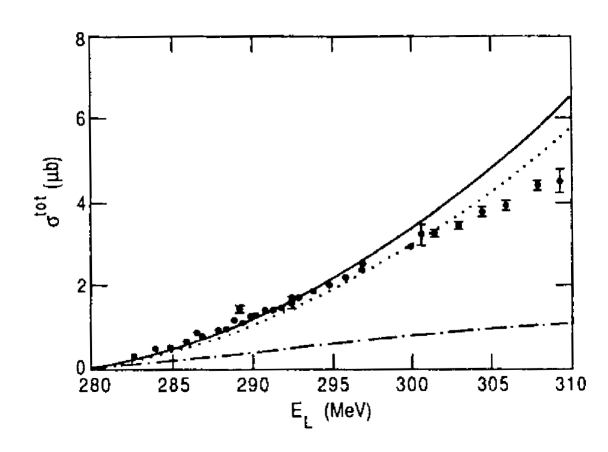
Figure 2.5: Cross section for $pp\rightarrow pp\pi^{0}$. The solid(dotted) line is the full calculation using the Bonn(Paris) potential to construct the axial exchange charge operator. The dot-dashed line is obtained by keeping only the one-body term of Eq. (2.6) and the pion re-scattering term of Eq. (2.10) using the Paris potential. The data points are from Refs. [21, 23]. Figure taken from Ref. [47].

As already found in previous works[38, 41], the impulse and re-scattering mechanism were not enough to describe the data (dot-dashed line of Fig. 2.5). The short-range axial charge operators enhance largely the cross section and remove most of the under prediction (solid and dotted lines of Fig. 2.5). However, it was also found that for both $NN$ potentials employed (Paris and Bonn), the energy dependence of the data was not reproduced in detail. According to Ref. [47], this might be due to the neglect of the energy dependence of the parameter $\lambda_{1}$ in the effective amplitude of Eq. (2.10), or to $p$-wave contributions and $\pi NN$ three-body scattering distortions in the final state. Although these corrections were expected to be small, they could in principle lead to significant contributions through the interference with large amplitudes and thus have large significant effects on the predicted energy dependence.

Shortly after the work of Ref. [47], where the meson-exchange contributions were calculated from phenomenological potentials, Ref. [48] used an explicit one-boson exchange model for the $NN$ interaction and for the calculation of the MEC’s. As in Ref. [47] the $\pi N$ re-scattering vertex was restricted however to the on-shell matrix element and to $s$-wave pion production. The largest contribution was found to come from the Z-diagrams mediated by $\sigma$-exchange, which was of the order of the one-body (impulse) term. The next important contribution was from the $\omega$ meson Z-diagrams ($35-45\%$ of the one-body term contribution).

The importance of off-shell effects

Shortly after the discovery of the importance of the short-range mechanisms, Hernández and Oset[51] demonstrated, using various parameterisations for the $\pi N\rightarrow\pi N$ transition amplitude, that its strong off-shell dependence could also be sufficient to remove the discrepancy between the Koltun and Reitan model[34] and the data.

The importance of the off-shell amplitudes was also seen in a relativistic one boson exchange model[52]. In the work of Ref. [53], the model independent off-shell $\pi N$ amplitude obtained by current algebra (and used previously in the Tucson-Melbourne three-nucleon force) was also considered as input for the pion re-scattering contribution to $pp\rightarrow pp\pi^{0}$ near threshold. It was found that this pion re-scattering contribution, together with the direct-production term, provided a good description of the $\pi^{0}$ production data, when the current algebra $\pi N$ amplitude parameters were updated with the phenomenological information obtained from the new meson factory $\pi N$ scattering data (see Fig. 2.6).

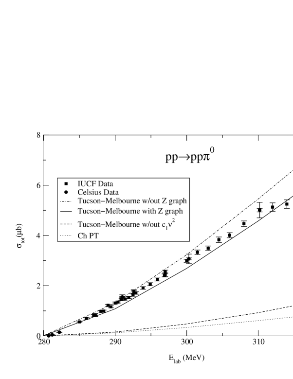
Figure 2.6: Cross section for $pp\rightarrow pp\pi^{0}$ using the Bonn B potential for the initial and final state interaction between the two protons. All calculations include both impulse and pion re-scattering diagrams. Figure taken from Ref. [53].

Z-diagrams: perturbative vs. non-perturbative

In the succeeding years many theoretical efforts were made for the calculation of the $pp\rightarrow pp\pi^{0}$ cross section. In Refs. [43, 54] covariant one boson exchange models were used in combination with an approximate treatment of the nucleon-nucleon interaction. Both models turned out to be dominated by heavy meson exchanges, thus giving further support to the picture proposed in Refs. [47, 48].

However, in Ref. [55] the negative energy nucleons were re-examined using the covariant spectator description, for both the production mechanism and for the initial and final state $pp$ interaction. This approach differs crucially from earlier ones by including non perturbatively the intermediate negative-energy states of the nucleons.

The perturbative result for the direct-production diagram was found to be about $3$ times larger that the non-perturbative one. Although the calculation in Ref. [55] did not include the re-scattering diagram contribution, it showed that the sensitive cross section for $\pi^{0}$ production seemed to be an ideal place to look for effects of relativistic dynamics.

The role of the nucleon resonances

Additional short-range contributions were also suggested, namely the $\rho-\omega$ meson exchange current[56], resonance contributions[56, 57, 58] (see Fig. 2.7) and loops that contain resonances[58]. All those, however, turned out to be smaller when compared to the heavy meson exchanges and the off-shell pion re-scattering.

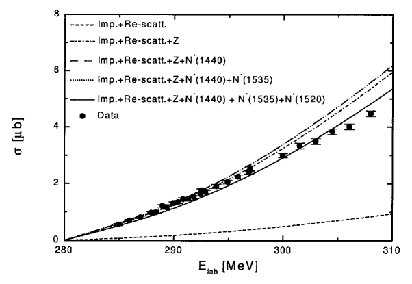
Figure 2.7: Total cross section for $pp\rightarrow pp\pi^{0}$ as a function of the proton laboratory energy. The net effect of the resonances is small. Figure taken from Ref. [57].

2.2 Coupled-channel phenomenological calculations

The starting point of the $NN$-$N\Delta$ approach is the recognition that the nucleon is a composite system. Since the $\Delta$ isobar is the most important mode of nucleonic excitation at intermediate energies, a possible process contributing (in second order) to nucleon-nucleon elastic scattering is the transition from a pure nucleonic state into a state into a nucleon plus a $\Delta$ (or two $\Delta$’s) with the inverse transition taking the system back to a two-nucleon state again. From this point of view, the nucleon-nucleon problem is a coupled-channel system involving at least the $NN$ and the $N\Delta$ channels[8].

2.2.1 The Hannover model

The Hannover model[18, 19, 20] for the $NN$ system considers the $\Delta$ isobar and pion degrees of freedom in addition to the nucleonic one. The model is based on a hamiltonian approach within the framework of non covariant quantum mechanics. In isospin-triplet partial waves, it extends the traditional approach with purely nucleonic potentials. It is constructed to remain valid up to $500\mathrm{MeV}$ CM energy. The Hilbert space considered comprises $NN$ and $N\Delta$ basis states, connected by transition potentials. Pion production and pion absorption are mediated by the $\Delta$ isobar excited by $\pi$ and $\rho$ exchange. The model accounts with satisfactory accuracy for the experimental data of elastic nucleon-nucleon scattering, of the inelastic reactions $pp\rightarrow\pi^{+}d$ and of elastic pion-deuteron scattering.

Lee and Matsuyama also performed calculations[15, 16, 17] for pion production within a coupled-channel approach, which differed from that of the Hannover group mainly by the treatment of the energy in the $\Delta$ propagator. Both the theoretical predictions[16, 19] from the Hannover and the Lee and Matsuyama models for the $pp\rightarrow pn\pi^{+}$ differential cross section were found to be quite sensitive to the inclusion of the $N\Delta$ potential, but the under-prediction of the data could not be completely removed. The calculations of Refs. [16, 19] considered an energy region well above pion production threshold ($\sim 580\mathrm{MeV}-800\mathrm{MeV}$), since pion production is assumed to occur only via an intermediate $\Delta$ excitation and thus the details of the $\pi N$ amplitude (related to chiral symmetry and the chiral limit), which are important close to threshold, were not included.

2.2.2 The Jülich model

The Jülich model[59, 60, 61] attempts to treat consistently the $NN$ and the $\pi N$ interaction for meson production close to threshold, taking both from microscopic models. Although not all parameters and approximations used in the two systems are the same, the same effective Lagrangians consistent with the symmetries of the strong interaction underlie the potentials to be used in the Lippmann-Schwinger equations for $NN$ and $\pi N$, independently. All single pion production channels including higher partial waves are considered.

The model used for the $NN$ distortions in the initial and final states is based on the Bonn potential[62]. The $\Delta$-isobar is treated in equal footing with the nucleons through a coupled-channel framework including the $NN$ as well as the $N\Delta$ and $\Delta\Delta$ channels. The model parameters were adjusted to the phase shifts below the pion production threshold.

Since all the short range mechanisms suggested in literature to contribute to pion production in $NN$ collisions mainly influence the production of $s$-wave pions, in the Jülich model only a single diagram was included (heavy meson through the $\omega$ as in diagram (d) of Fig. 2.1) to parameterise these various effects. The strength of this contribution was adjusted to reproduce the total cross section of the reaction $pp\rightarrow pp\pi^{0}$ close to threshold. After this is done, all the parameters are fixed.

The model describes qualitatively the data, as shown in Fig. 2.8. The most striking differences appear for double polarisation observables in the neutral pion channel. As a general pattern the amplitudes seem to be of the right order of magnitude, but show a wrong interference pattern.

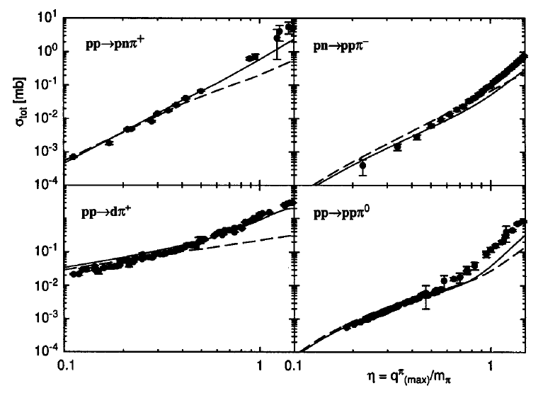
Figure 2.8: Comparison of the Jülich phenomenological model of [59, 60, 61] to the data. The solid lines show the result of the full model and the dashed lines show the results without the $\Delta$ contributions. Figure taken from Ref. [3].

For charged pion production most of observables are described satisfactorily. In contrast to the neutral channel, the charged pion production was found to be completely commanded by two transitions, namely, ${}^{3}P_{1}\rightarrow^{3}S_{1}s$, which is dominated by the isovector pion re-scattering, and ${}^{1}D_{2}\rightarrow^{3}S_{1}p$, which governs the cross section especially in the regime of the $\Delta$ resonance.

2.3 Chiral perturbation theory

In the late 90’s there was the hope that $\chi$PT might resolve the true ratio of re-scattering and short-range contributions in pion production. It came as a big surprise, however, that the first results for the reaction $pp\rightarrow pp\pi^{0}$ [36, 63] showed that the $\chi$PT $\pi N$ scattering amplitude interfered destructively with the direct contribution, making the discrepancy with the data even more severe, and thus suggesting a significant role for heavy meson exchanges in $\pi^{0}$ production[64, 65]. In addition, the same isoscalar re-scattering amplitude also worsened the discrepancy in the $\pi^{+}$ channel[66].

In low-energy pion physics, the constrains to an effective field theory ($\chi$PT) come from chiral symmetry, since it forces not only the mass of the pion to be low, but also the interactions to be weak: the pion needs to be free of interactions in the chiral limit for vanishing momenta. The first success of $\left(\chi\text{Pt}\right)$ was the application to meson-meson scattering[67]. Treating baryons as heavy allowed straightforward extension of the scheme to meson-baryon[68] as well as baryon-baryon systems[69, 70, 71, 72]. The $\Delta$ isobar could also be included consistently in the effective field theory[73]. It was shown recently[74, 75] that when the new scale induced by the initial momentum $p\sim\sqrt{m_{\pi}M}$ for meson production in nucleon-nucleon collisions is taken properly into account, the series indeed converges.

The starting point for the derivation of the amplitude is an appropriated Lagrangian density, constructed to be consistent with the symmetries of QCD and ordered according to a particular counting scheme. The leading order Lagrangian is[3, 66, 68]

$$\mathcal{L}^{\left(0\right)} = \frac{1}{2}\partial_{\mu}\boldsymbol{\pi}\partial^{\mu}\boldsymbol{\pi}-\frac{1}{2}m_{\pi}^{2}\boldsymbol{\pi}^{2}+\frac{1}{f_{\pi}^{2}}\left[\left(\boldsymbol{\pi}\cdot\partial_{\mu}\boldsymbol{\pi}\right)^{2}-\frac{1}{4}m_{\pi}^{2}\left(\boldsymbol{\pi}^{2}\right)^{2}\right]$$

$$+N^{\dagger}\left[i\partial_{0}-\frac{1}{4f_{\pi}^{2}}\boldsymbol{\tau}\cdot\left(\boldsymbol{\pi}\times\boldsymbol{\dot{\pi}}\right)+\frac{g_{A}}{2f_{\pi}}\boldsymbol{\tau}\cdot\vec{\sigma}\cdot\left(\vec{\nabla}\boldsymbol{\pi}+\frac{1}{2f_{\pi}^{2}}\boldsymbol{\pi}\left(\boldsymbol{\pi}\cdot\vec{\nabla}\boldsymbol{\pi}\right)\right)\right]N$$

$$+\Psi_{\Delta}^{\dagger}\left(i\partial_{0}-\Delta\right)\Psi_{\Delta}+\frac{h_{A}}{2f_{\pi}}\left[N^{\dagger}\left(\boldsymbol{T}\boldsymbol{\cdot}\vec{S}\boldsymbol{\cdot}\vec{\nabla}\boldsymbol{\pi}\right)\Psi_{\Delta}+h.c.\right]+...$$

and the next-to-leading order Lagrangian is

$$\mathcal{L}^{\left(1\right)} = \frac{1}{2M}\left[N^{\dagger}\vec{\nabla}^{2}N+\Psi_{\Delta}^{\dagger}\vec{\nabla}^{2}\Psi_{\Delta}\right]+\frac{1}{8Mf_{\pi}^{2}}\left[iN^{\dagger}\boldsymbol{\tau}\boldsymbol{\cdot}\left(\boldsymbol{\pi}\times\vec{\nabla}\boldsymbol{\pi}\right)\boldsymbol{\cdot}\vec{\nabla}N+h.c.\right]$$

$$+\frac{1}{f_{\pi}^{2}}N^{\dagger}\left[\left(c_{2}+c_{3}-\frac{g_{A}^{2}}{8M}\right)\boldsymbol{\dot{\pi}}^{2}-c_{3}\left(\vec{\nabla}\boldsymbol{\pi}\right)^{2}-2c_{1}m_{\pi}^{2}\boldsymbol{\pi}^{2}\right.$$

$$\left.-\frac{1}{2}\left(c_{4}+\frac{1}{4M}\right)\epsilon_{ijk}\epsilon_{abc}\sigma_{k}\boldsymbol{\tau}_{c}\partial_{i}\boldsymbol{\pi}_{a}\partial_{j}\boldsymbol{\pi}_{b}\right]N+\frac{\delta}{2}N^{\dagger}\left[\tau_{3}-\frac{1}{2f_{\pi}^{2}}\pi_{3}\boldsymbol{\pi}\cdot\boldsymbol{\boldsymbol{\tau}}\right]N$$

$$-\frac{g_{A}}{4Mf_{\pi}}\left[iN^{\dagger}\boldsymbol{\tau}\boldsymbol{\cdot\dot{\pi}}\vec{\sigma}\boldsymbol{\cdot}\vec{\nabla}N+h.c.\right]-\frac{h_{A}}{2Mf_{\pi}}\left[iN^{\dagger}\boldsymbol{T}\boldsymbol{\cdot\dot{\pi}}\vec{S}\boldsymbol{\cdot}\vec{\nabla}\Psi_{\Delta}+h.c.\right]$$

$$-\frac{d_{1}}{f_{\pi}}N^{\dagger}\left(\boldsymbol{\tau}\cdot\vec{\sigma}\cdot\vec{\nabla}\boldsymbol{\pi}\right)NN^{\dagger}N-\frac{d_{2}}{2f_{\pi}}\epsilon_{ijk}\epsilon_{abc}\partial_{i}\boldsymbol{\pi}_{a}N^{\dagger}\sigma_{j}\boldsymbol{\tau}_{b}NN^{\dagger}\sigma_{k}\boldsymbol{\tau}_{c}N+...$$

where $f_{\pi}$ is the pion decay constant in the chiral limit, $g_{A}$ is the axial-vector coupling of the nucleon and $h_{A}$ is the $\Delta N\pi$ coupling. The the nucleon, pion and $\Delta$ field are $N$, $\pi$ and $\Psi_{\Delta}$, respectively. The isobar-nucleon mass difference is $\Delta$, and the quark mass difference contribution to the neutron-proton mass difference is $\delta$. The $1/2\rightarrow 3/2$ spin transition matrix operator is $\vec{S}$ and the $1/2\rightarrow 3/2$ isospin transition matrix operator is $\boldsymbol{T}$. The are normalised such that

$$S_{i}S_{j}^{\dagger}=\frac{1}{3}\left(2\delta_{ij}-i\epsilon_{ijk}\sigma_{k}\right)\hskip 71.13188ptT_{i}T_{j}^{\dagger}=\frac{1}{3}\left(2\delta_{ij}-i\epsilon_{ijk}\tau_{k}\right).$$ (2.13)

The constants $c_{i}$, not constrained by chiral symmetry, depend on the details of QCD dynamics. They are at present unknown functions of the fundamental QCD parameters, and can be extracted from a fit to elastic $\pi N$ scattering. The corresponding values are in Table 2.1. In a theory without explicit $\Delta$’s, their effect is absorbed in the low energy constants (see Fig. 2.9), which is called resonance saturation (infinitely heavy or static limit). Thus, in the case of a theory which considers explicit $\Delta$’s, the $\Delta$ contribution needs to be subtracted from the values given in the first two columns of Table 2.1.

$i\hskip 12.80365pt$	$c_{i}^{\text{tree}}$	$c_{i}^{\text{loop}}$	$c_{i}^{\text{tree}}\left(\not\Delta\right)$	$c_{i}^{\text{loop}}\left(\not\Delta\right)$
$1\hskip 12.80365pt$	$-0.64$	$-0.93$	$-0.64$	$-0.93$
$2\hskip 12.80365pt$	$1.78$	$3.34$	$0.92$	$0.64$
$3\hskip 12.80365pt$	$-3.90$	$-5.29$	$-1.20$	$-2.59$
$4\hskip 12.80365pt$	$2.25$	$3.63$	$0.90$	$2.28$

Table 2.1: Low-energy constants $c_{i}$ for $\mathcal{L}^{\left(0\right)}$ and $\mathcal{L}^{\left(1\right)}$ of Eq. (2.3)-Eq. (2.3) (in $\mathrm{GeV}^{-1}$). The first two columns are from Ref. [77] and Ref. [76]. The last two columns are obtained subtracting a chosen $\Delta$ contribution of $c_{2}^{\Delta}=-c_{3}^{\Delta}=2c_{4}^{\Delta}=2.7\mathrm{GeV}^{-1}$ [3].

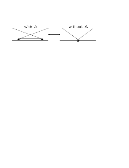
Figure 2.9: Illustration of resonance saturation. Figure taken from Ref. [3].

2.3.1 Power counting for the impulse term

Within the framework of $\chi$PT, only pion exchange is considered. Also, the impulse term (Fig. 2.1 (a)) is included in the class of irreducible diagrams defined in Weinberg’s sense. A sub-diagram is considered reducible in Weinberg’s sense if it includes a small energy denominator of the order of $\sim m_{\pi}^{2}/M$ and irreducible otherwise[63]. In the following, we present the power counting for the impulse term.

Since near threshold the pion carries an energy of the order of the pion mass, at least one of the nucleon intermediate states, before or after pion emission, must be off mass-shell by $\sim m_{\pi}$. The transition to an off-mass-shell state is induced by a relatively high-momentum $\left(\sim\sqrt{m_{\pi}M}\right)$ meson exchange mechanism. Therefore, the irreducible sub-diagrams of Fig. 2.1 (a) are in lowest order to be drawn as in Fig. 2.10.

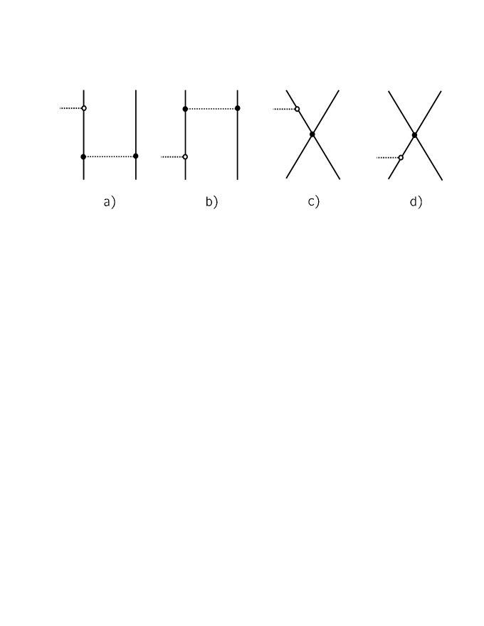
Figure 2.10: Diagrams contributing to the impulse term that are irreducible in the context of chiral power counting for the $pp\rightarrow pp\pi^{0}$ reaction. The solid and dotted lines denote the nucleons and the pions, respectively. Leading(sub-leading) vertices are represented by solid(open) circles. They are originated by the three-momentum(energy) dependence of the vertex.

The corresponding power counting is done as follows:

• Close to threshold, the $\vec{\sigma}\cdot\vec{q}$ term of the $\pi NN$ vertex is suppressed, and the pion-nucleon interaction proceeds via the Galilean term $\left[N^{\dagger}\boldsymbol{\tau}\boldsymbol{\cdot\dot{\pi}}\vec{\sigma}\boldsymbol{\cdot}\vec{\nabla}N\right]$ of Eq. (2.3). This yields a factor of

  $$\frac{1}{f_{\pi}}\frac{pE_{\pi}}{M}\sim\frac{\sqrt{Mm_{\pi}}m_{\pi}}{f_{\pi}M}=\frac{m_{\pi}^{3/2}}{f_{\pi}M^{1/2}}.$$ (2.14)

• Since the nucleon-nucleon interaction originates from virtual (static) pion exchange, as in Fig. 2.10 (a) and (b), each three-momentum dependent $\pi NN$ vertex contributes with a factor of $\sqrt{m_{\pi}M}/f_{\pi}$ and the pion propagator contributes with a factor of $\left(m_{\pi}M\right)^{-1}$, thus giving the overall factor of $f_{\pi}^{-2}$ from the nucleon-nucleon interaction. If the nucleon-nucleon interaction arises from exchange of a heavier meson, as in Fig. 2.10 (c) and (b), the overall factor is also $\left(\frac{g_{NNh}}{m_{h}}\right)^{2}\sim\frac{1}{f_{\pi^{2}}}$.

• Near threshold, the contribution of the non-relativistic two-nucleon propagator is $\left(E_{\mathrm{intermediate}}-E_{\mathrm{initial}}\right)^{-1}\sim m_{\pi}^{-1}$.

• Finally, the overall contribution of the impulse term is then

  $$\frac{m_{\pi}^{3/2}}{f_{\pi}M^{1/2}}\times\frac{1}{f_{\pi}^{2}}\frac{1}{m_{\pi}}=\frac{1}{f_{\pi}^{3}}\sqrt{\frac{m_{\pi}}{M}}.$$ (2.15)

In conclusion, the impulse term is not irreducible in the Weinberg’s sense. Within $\chi$PT the impulse term is calculated as given by the (distorted) diagrams in Fig. 2.10.

2.3.2 Why $\pi^{0}$ is problematic

For neutral pion production there is no meson exchange operator at leading order and the nucleonic operator gets suppressed by the poor overlap of the initial and final state wave functions (an effect not captured by the power counting) and interferes destructively with the direct production of the $\Delta$. Thus the first significant contributions appear at NNLO. As there is a large number of diagrams at NNLO, the different short-range mechanisms found in the literature and discussed before are of similar importance and capable of removing the discrepancy between the Koltun and Reitan result and the data. Charged pion production is expected to be significantly better under control, since there is a meson exchange current at leading order and there are non-vanishing loop contributions[66].

The importance of the pion loops

The most prominent diagram for neutral pion production close to threshold is the pion re-scattering via the isoscalar $T$-matrix that, for the kinematics given, is dominated by one-sigma exchange[3]. Within the effective field theory the isoscalar potential is built up perturbatively. The leading piece of the one-sigma exchange gets cancelled by other loops that cannot be interpreted as a re-scattering diagram and therefore are not included in the phenomenological approaches. This is an indication that in order to improve the phenomenological approaches, at least in case of neutral pion production, pion loops should be considered as well.

2.3.3 Charged pion production in $\chi$PT

The main calculations on $pp\rightarrow pn\pi^{+}$ in the framework of $\chi$PT are those of Ref. [66], which also included the mechanism proposed in Refs. [47, 48], where the short-range interaction is supposed to be originated from $Z$-diagrams mediated by $\sigma$ and $\omega$ changes. The Coulomb interaction is disregarded in the $pn\pi^{+}$ final state. The channels considered were ${}^{3}P_{1}\rightarrow\left({}^{3}S_{1}\right)p$ and ${}^{3}P_{0}\rightarrow\left({}^{1}S_{0}\right)s$. For the ${}^{3}S_{1}$ final state, the Weinberg-Tomozawa term contribution is found to be the largest. Most of the other contributions were much smaller and tended to cancel each other to some extent. The exception was the $\Delta$ contribution which had a significant destructive interference with the Weinberg-Tomozawa term. Although the theory produces the correct shape for the $\eta$ dependence, it fails in magnitude by a factor of $\sim 5$ (see Fig. 2.11).

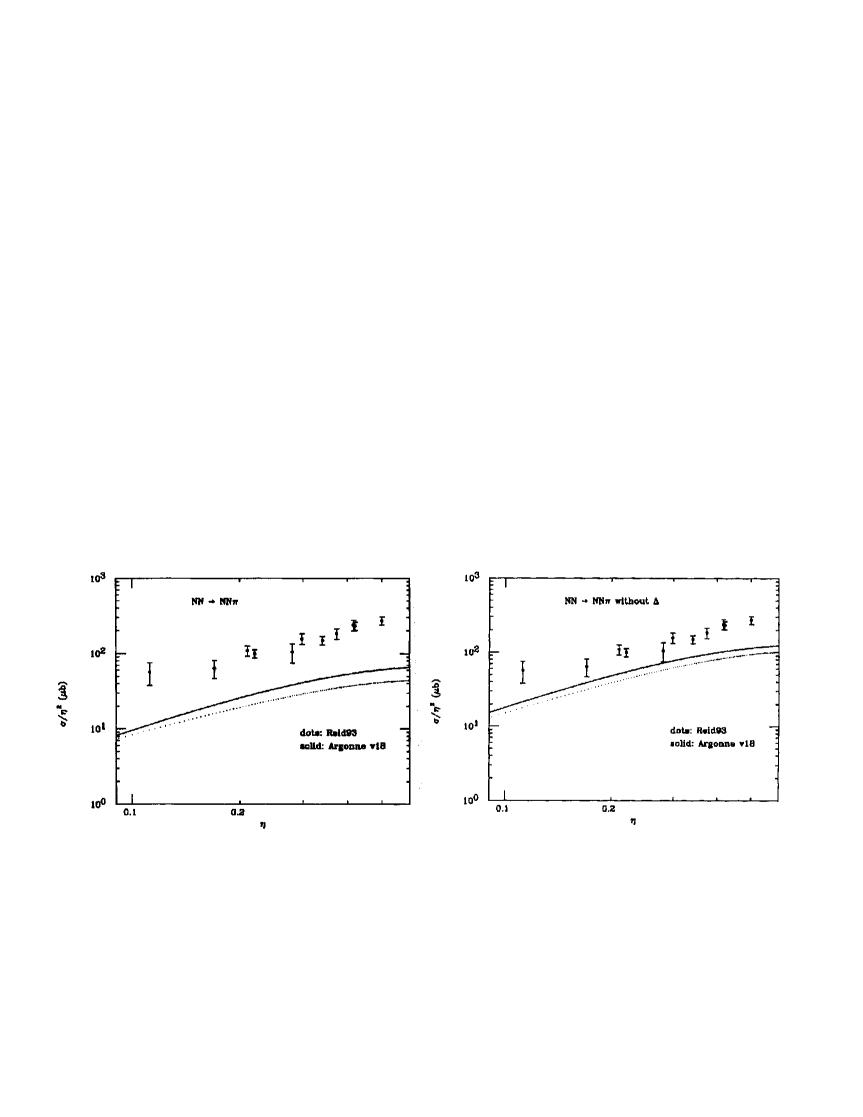
Figure 2.11: Reduced cross section for $pp\rightarrow pn\pi^{+}$ with (left panel) and without (right panel) the $\Delta$ contribution. The dotted and solid lines correspond, respectively to the Reid 93 and Argonne 18 $NN$ potentials. Figure taken from Ref. [66].

Ref. [66] suggested that the $\Delta$ contribution may be overestimated by a factor of $50\%$ or more. Actually, the cross sections with and without the $\Delta$ contribution (respectively, left and right panel of Fig. 2.11), differed by almost a factor of $2$. This could arise from the uncertainties on the $\pi N\Delta$ coupling constant, or from the neglecting of the $\Delta$-$N$ mass difference in energies. The kinetic energy of the $\Delta$ was also neglected, account of which would further decrease its amplitude.

2.3.4 The $V_{\mathrm{low-k}}$ approach

As there are no $\chi$PT $NN$ potentials available yet for pion production calculations, in practices one usually uses a hybrid (not much consistent) $\chi$PT approach, in which the transition operators are derived from $\chi$PT but the nuclear wave functions are generated from high-precision phenomenological $NN$ potentials. However, a conceptual problem underlying these hybrid $\chi$PT calculations is that, whereas the transition operators are derived assuming that relevant momenta are sufficient small compared with the chiral scale $\chi\sim 1\mathrm{GeV}$, the wave functions generated by a phenomenological potential can in principle contain momenta of any magnitude[78].

A systematic method based on the renormalisation group approach was recently developed[79] to construct from a phenomenological “bare” $NN$ potential an effective $NN$ potential, $V_{\mathrm{low-k}}$, by integrating out momentum components above a specified cutoff scale $\Lambda$. For a $\Lambda=2.1\mathrm{fm}^{-1}$, it was found[79] that the low momentum behaviour of the $NN$ wave functions calculated from $V_{\mathrm{low-k}}$ is essentially model independent.

The very recent first calculation[78] for $pp\rightarrow pp\pi^{0}$ using the $V_{\mathrm{low-k}}$ approach led to a cross section closer to the experimental data than the one calculated with “bare” potentials.

2.4 Energy prescription for the exchanged pion

In most of the calculations on pion production, several approximations to the pion production vertex and the kinematics have been tacitly assumed from the very first investigation by Koltun and Reitan[34]. However, these prescriptions were found to have a significant effect both in the magnitude and energy dependence of the cross section[57, 59, 80], as it is illustrated by Fig. 2.12 and by Fig. 2.13.

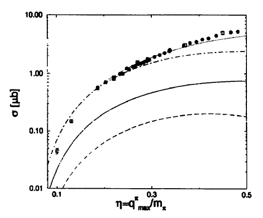
Figure 2.12: Cross section for $pp\rightarrow pp\pi^{0}$. The solid curve is the full calculation of the re-scattering and direct production diagrams whereas the dashed line corresponds to the direct production diagram only. The dashed-dotted curve is the full result scaled by a factor of $\sim 4$. The dotted curve is the full calculation with the approximate treatment of the pion production vertex of Ref. [51] (frozen kinematics). Figure taken from Ref. [59].

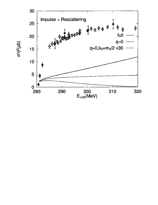
Figure 2.13: Cross section for $pp\rightarrow pp\pi^{0}$, including both impulse and re-scattering amplitudes. The solid line is the calculation assuming four-momentum conservation and that the intermediate particles are on-mass-shell. The dotted and dashed-dotted lines correspond to two different fixed-threshold prescriptions for the energy of the exchanged pion. Figure taken from Ref. [80].

Fig. 2.12 refers to the calculations[59] for $pp\rightarrow pp\pi^{0}$ based on the Jülich model presented in Sec. 2.2. It differs from the calculation of Ref. [51] since the momentum of the exchanged pion is not fixed to the value corresponding to the particular kinematic situation at the pion production threshold when there are no distortions in the initial and final $pp$ states.

The full treatment of the pion production vertex (solid line of Fig. 2.12) reduced the $\pi^{0}$ production rate by a factor of $2$. Therefore, the work of Ref. [59] concluded that the enhancement of the re-scattering amplitude due to offshellness falls a bit too short to explain the scale of the $pp\rightarrow pp\pi^{0}$ cross section.

In Fig. 2.13 we show a calculation for the $pp\rightarrow pp\pi^{0}$ reaction within $\chi$PT, which also aimed to investigate the effect of the simplifying assumptions on the energy-momentum flow in the re-scattering diagram[80]. For this case, the discrepancy between the approximations was found to be of a factor of $3$.

A clarification of these formal issues is thus necessary before one can draw conclusions about the physics of the pion production processes. More specifically, one needs to obtain a three-dimensional formulation from the more general Feynman procedure. This will be the subject of the next Chapter, and was the starting point of this thesis work.

Chapter 3 From Field Theory to DWBA

Abstract: DWBA calculations, which are currently applied to pion production, are based on a quantum-mechanical three-dimensional formulation for the initial- and final-$NN$ distortion, which is not obtained from the four-dimensional field-theoretical Feynman diagrams. As a consequence, the energy of the exchanged pion has been treated approximately in the calculations performed so far. This Chapter will discuss the validity of the DWBA approach through the link with the time-ordered perturbation theory diagrams which result from the decomposition of the corresponding Feynman diagram.

All the meson production mechanisms described in the previous Chapter are derived from relativistic Feynman diagrams. Nevertheless, within the framework of DWBA, the evaluation of the corresponding matrix elements for the cross section proceeds through non-relativistic initial and final nucleonic wave functions. Therefore the calculations apply a three-dimensional formulation in the loop integrals for the nucleonic distortion, which is not obtained from the underlying field-theoretical Feynman diagrams. Namely, the energy of the exchanged pion in the re-scattering operator (both in the $\pi N$ amplitude and in the exchanged pion propagator) has been treated approximately and under different prescriptions in calculations performed till now. In other words, the usual approach, as in Refs. [36, 56, 57, 63, 66, 81], is to use an educated “guess” for the energy-dependence of the virtual pion-nucleon interaction and then to use a Klein-Gordon propagator for the exchanged pion propagator. In particular, most of the calculations assume a typical threshold kinematics situation even when the exchanged pion is expected to be largely off-shell.

A theoretical control of the energy for the loop integration embedding the non-relativistic reduction of the Feynman $\pi$-exchange diagram in the non-relativistic nucleon-nucleon wave functions became then an important issue, as pointed out in Refs. [82, 83].

In this Chapter, following the work of Ref. [84], we deal with the isoscalar re-scattering term for the $pp\rightarrow pp\pi^{0}$ reaction (near threshold). Although for $\pi^{0}$ production, as mentioned in Chapter 2, the re-scattering mechanism is indeed small, the amount of its interference with the (also small) impulse term depends quantitatively on the calculation method. We note, furthermore, that the pion isoscalar re-scattering term, which is energy dependent, increases away from threshold, and that for the charged pion production reactions the isovector term is important, and also depends on the exchanged pion energy. Thus the knowledge gained from the application discussed here to the $pp\rightarrow pp\pi^{0}$ reaction near threshold is useful for other applications.

Specifically, this Chapter will focus on the investigation of

• the validity of the traditionally employed DWBA approximation. We will use as a reference the result obtained from the decomposition of the Feynman diagram into TOPT diagrams, and realise how the last ones link naturally to an appropriate quantum-mechanical DWBA matrix element. This study for a realistic $\pi NN$ coupling was not done before;

• the (numerical) importance of the three-body logarithmic singularities of the exact propagator of the exchanged pion, which are not present when the usual approximations in DWBA are considered; this study was not done before.

The work of Ref. [84] generalised the work of Refs. [82, 83] which considered a solvable toy model for scalar particles and interactions and treated the nucleons as distinguishable and therefore pion emission to proceed only from one nucleon. It is described by the following Lagrangian

$$\mathcal{L} = \sum_{i=1,2}N_{i}^{\dagger}\left(i\partial_{0}+\frac{\nabla^{2}}{2M}\right)N_{i}+\frac{1}{2}\left[\left(\partial_{\mu}\pi\right)^{2}-m_{\pi}^{2}\pi^{2}\right]+\frac{1}{2}\left[\left(\partial_{\mu}\sigma\right)^{2}-m_{\sigma}^{2}\sigma^{2}\right]+$$ (3.1)

$$\frac{g_{\pi}}{f_{\pi}}N_{2}^{\dagger}N_{2}\pi+g_{\sigma}\sum_{i=1,2}N_{i}^{\dagger}N_{i}\sigma+\frac{c}{f_{\pi}^{2}}\sum_{i=1,2}N_{i}^{\dagger}N_{i}\left(\partial_{0}\pi\right)^{2}$$

where $N_{i}$ and $\pi$ are the nucleon and pion field, respectively. Eq. (3.1) further assumes a Yukawa coupling for the pion-nucleon coupling, $\frac{g_{\pi}}{f_{\pi}}$ and describes the pion re-scattering through a $\pi N$ seagull vertex inspired by the chiral $\pi N$ interaction Lagrangian of Eq. (2.3), $\frac{c}{f_{\pi}^{2}}Q_{0}^{\prime}Q_{0}$, where $c$ is an arbitrary constant. In this toy model, the nuclear interactions are described through $\sigma$-exchange, which also couples to the nucleons via a Yukawa coupling, $g_{\sigma}$, and the nucleons are treated non-relativistically (in particular, contributions from nucleon negative-energy states are not considered).

There are some nonrealistic features of this model that also motivated our work and the one of Ref. [84]. First of all, the model does not satisfy chiral symmetry, which would have required a derivative coupling of the pion to the nucleon instead of the simpler Yukawa coupling. Furthermore, in this toy model the nucleons, interacting via $\sigma$ exchange, have a stronger overlap than in a more realistic model, since it does not include short-range repulsive nucleon-nucleon interactions that keep the nucleons apart. Note also that near threshold kinematics, the scalar particle is produced in a $s$-wave state, as is the final nucleon-nucleon pair (and the initial nucleon -nucleon pair too, by angular momentum conservation requirements). This is not the case for the production of a real pion, since it is a pseudo-scalar particle and, therefore, near threshold the production of $s$-wave pions calls for a initial $P$-wave nucleon state.

Our calculation employs a physical model for nucleons and pions and investigates how much of the features found in Refs. [82, 83] survive in a more realistic calculation which uses a pseudo-vector coupling for the $\pi NN$ vertex, the $\chi$PT $\pi N$ amplitude[36] and the Bonn B potential[62] for the nucleon-nucleon interaction.

3.1 Extraction of the effective production operator

3.1.1 Final-state interaction diagram

The amplitude

The Feynman diagram for the reaction $pp\rightarrow pp\pi^{0}$ where the $NN$ final-state interaction (FSI) proceeds through sigma exchange is represented in part $a$ of Fig. 3.3. After the nucleon negative-energy states are neglected, it corresponds to the amplitude

$$\mathcal{M}_{FSI}= ig_{\sigma}^{2}\int\frac{d^{4}Q^{\prime}}{\left(2\pi\right)^{4}}f\left(Q_{0}^{\prime}\right)\frac{1}{Q_{1}^{0}-\omega_{1}+i\varepsilon}\frac{1}{Q_{2}^{0}-\omega_{2}+i\varepsilon}\frac{1}{K_{0}^{2}-\omega_{\sigma}^{2}+i\varepsilon}$$

$$\frac{1}{Q_{0}^{\prime 2}-\omega_{\pi}^{2}+i\varepsilon}$$

where the exchanged pion has four-momentum $Q^{\prime}=\left(Q^{\prime}_{0},\vec{q}^{\,\prime}\right)$. The four-momenta of the intermediate nucleons are $Q_{1}$ and $Q_{2}$ and the four-momentum of the exchanged $\sigma$ is $K$. The on-mass-shell energies for the intermediate nucleons, exchanged pion and sigma mesons are $\omega_{1,2}$, $\omega_{\pi}$, $\omega_{\sigma}$, respectively. In Appendix B details on these functions are given. All quantities are referred to the three-body centre-of-mass frame of the $\pi NN$ final state.

In Eq. (3.1.1) $f\left(Q_{0}^{\prime}\right)$ is a short-hand notation for both the $\mathcal{M}_{\pi NN}$ and $\mathcal{M}_{\pi\pi NN}$. We note that $f$ in fact may depend on the three-momenta and energies of both the exchanged and produced pion, and also on the nucleon spin. However, for simplicity, only the dependence on the energy of the exchanged pion, $Q^{\prime}_{0}$, is emphasised, because this is the important variable for the main considerations of these Chapter. For the toy model described by the lagrangian of Eq. (3.1), it is

$$f\left(Q_{0}^{\prime}\right)=\left(\frac{g_{\pi}}{f_{\pi}}\right)\times\left(\frac{c}{f_{\pi}^{2}}Q_{0}^{\prime}E_{\pi}\right)\text{,}$$ (3.3)

but for the more realistic case of Ref. [84] which uses a pseudo-vector coupling for the $V_{\pi NN}$ vertex and the $\chi$PT $\pi N$ amplitude[36], it reads

$$f\left(Q_{0}^{\prime}\right)=\left(\frac{g_{A}}{f_{\pi}}\vec{\sigma}^{2}\cdot\vec{q}^{\,\prime}\right)\times\frac{m_{\pi}^{2}}{f_{\pi}^{2}}\left[2c_{1}+\left(c_{2}+c_{3}-\frac{g_{A}^{2}}{8M}\right)\frac{E_{\pi}Q_{0}^{\prime}}{m_{\pi}^{2}}+c_{3}\frac{\vec{q}^{\prime}\cdot\vec{q}_{\pi}}{m_{\pi}^{2}}\right]$$ (3.4)

In Eq. (3.3) and Eq. (3.4), $E_{\pi}$$\left(\vec{q}_{\pi}\right)$ is the energy (three-momentum) of the produced pion. As mentioned before, $f_{\pi}$ is the pion decay constant and $g_{A}$ is the nucleon axial vector coupling constant, which is related to the pseudovector coupling constant $f_{\pi NN}$ by the Goldberger-Treiman relation $\frac{g_{A}}{2f_{\pi}}=\frac{f_{\pi NN}}{m_{\pi}}$. The low-energy constants $c_{i}^{\prime}$s are defined on Table 2.1.

Using four-momentum conservation, the amplitude of Eq. (3.1.1) can be written as

$$\mathcal{M}_{FSI} = -ig_{\sigma}^{2}\int\frac{d^{4}Q^{\prime}}{\left(2\pi\right)^{4}}f\left(Q_{0}^{\prime}\right)\frac{1}{E_{1}+Q_{0}^{\prime}-E_{\pi}-\omega_{1}+i\varepsilon}\frac{1}{Q_{0}^{\prime}-E_{2}+\omega_{2}-i\varepsilon}$$

$$\frac{1}{F_{2}-E_{2}+Q_{0}^{\prime}-\omega_{\sigma}+i\varepsilon}\frac{1}{F_{2}-E_{2}+Q_{0}^{\prime}+\omega_{\sigma}-i\varepsilon}\frac{1}{Q_{0}^{\prime}-\omega_{\pi}+i\varepsilon}\frac{1}{Q_{0}^{\prime}+\omega_{\pi}-i\varepsilon}$$

where the functions $E_{1,2}$$\left(F_{1,2}\right)$ stand for the energy of the initial(final) nucleons.

The integrand in Eq. (3.1.1) has three poles in the upper half-plan and three poles in lower half-plan. They are schematically reproduced on Fig. 3.1.

Figure 3.1: Schematic position (scaled for a kinematics close to pion production threshold) of the poles in $Q^{\prime}_{0}$ of the amplitude of Eq. (3.1.1). The diamonds, open circles and bullets represent, the nucleon poles, the sigma poles and the pion poles, respectively.

To integrate Eq. (3.1.1) over the energy variable $Q^{\prime}_{0}$ we can close the contour on one of the half-planes and pick each of the three poles enclosed. However, to get a more straightforward connection with the DWBA formalism through time-ordered perturbation theory, it is better to perform a partial fraction decomposition to isolate the pion poles before integrating over $Q_{0}^{\prime}$. All details of this decomposition are given in Appendix C.

As a result, Eq. (3.1.1) is expressed as a sum of eight types of terms, with each one having at the maximum three poles, as represented in Fig. 3.2. From this figure one realises that only $4$ terms do not vanish after the $Q^{\prime}_{0}$ integration: they correspond to the location of the poles as represented in the last $4$ diagrams of Fig. 3.2.

Figure 3.2: Schematic position of the poles in $Q^{\prime}_{0}$ resulting from the partial fraction decomposition of the amplitude of Eq. (3.1.1). The meaning of the symbols is the same of Fig. 3.1.

After the $Q^{\prime}_{0}$ integration, one obtains for Eq. (3.1.1):

$$\mathcal{M}^{FSI}_{TOPT}=-g_{\sigma}^{2}\int\frac{d^{3}q^{\prime}}{\left(2\pi\right)^{3}}\frac{1}{4\omega_{\sigma}\omega_{\pi}}\times$$ (3.6)

$$\left[\frac{f\left(\omega_{\pi}\right)}{\left(E_{tot}-E_{\pi}-\omega_{1}-\omega_{2}\right)\left(E_{tot}-E_{1}-\omega_{2}-\omega_{\pi}\right)\left(E_{tot}-F_{1}-E_{\pi}-\omega_{2}-\omega_{\sigma}\right)}\right.$$

$$\left.+\frac{f\left(\omega_{\pi}\right)}{\left(E_{tot}-E_{\pi}-\omega_{1}-\omega_{2}\right)\left(E_{tot}-E_{1}-\omega_{2}-\omega_{\pi}\right)\left(E_{tot}-F_{2}-E_{\pi}-\omega_{1}-\omega_{\sigma}\right)}\right.$$

$$\left.+\frac{f\left(-\omega_{\pi}\right)}{\left(E_{tot}-E_{\pi}-\omega_{1}-\omega_{2}\right)\left(E_{tot}-E_{2}-E_{\pi}-\omega_{1}-\omega_{\pi}\right)\left(E_{tot}-F_{1}-E_{\pi}-\omega_{2}-\omega_{\sigma}\right)}\right.$$

$$\left.+\frac{f\left(-\omega_{\pi}\right)}{\left(E_{tot}-E_{\pi}-\omega_{1}-\omega_{2}\right)\left(E_{tot}-E_{2}-E_{\pi}-\omega_{1}-\omega_{\pi}\right)\left(E_{tot}-F_{2}-E_{\pi}-\omega_{1}-\omega_{\sigma}\right)}\right.$$

$$\left.+\frac{f\left(\omega_{\pi}\right)}{\left(E_{tot}-E_{1}-\omega_{2}-\omega_{\pi}\right)\left(E_{tot}-F_{2}-E_{\pi}-\omega_{1}-\omega_{\sigma}\right)\left(E_{tot}-E_{1}-F_{2}-\omega_{\pi}-\omega_{\sigma}\right)}\right.$$

$$\left.+\frac{f\left(-\omega_{\pi}\right)}{\left(E_{tot}-E_{2}-E_{\pi}-\omega_{1}-\omega_{\pi}\right)\left(E_{tot}-F_{1}-E_{\pi}-\omega_{2}-\omega_{\sigma}\right)\left(E_{tot}-E_{2}-F_{1}-E_{\pi}-\omega_{\pi}-\omega_{\sigma}\right)}\right]$$

with $E_{tot}=2E=F_{1}+F_{2}+E_{\pi}$ and $E\equiv E_{1}=E_{2}$.

This equation evidences that there are six contributions to the amplitude. These six terms, originated by the four propagators of the loop, can be interpreted as time-ordered diagrams. They are represented by diagrams $a_{1}$ to $a_{6}$ in Fig. 3.3. This interpretation justifies the extra subscript label $TOPT$ for the $\mathcal{M}_{FSI}$ amplitude in Eq. (3.6).

Figure 3.3: Decomposition of the Feynman diagram in terms of six time-ordered diagrams for the final-state interaction. The pion(sigma) field is represented by a dashed(solid double) line. The nucleons are represented by solid lines. The DWBA amplitude may be identified to the first four time-ordered diagrams ($a_{1}$ to $a_{4}$). The last two diagrams ($a_{5}$ to $a_{6}$) are usually called stretched boxes.

Obviously, the result of direct integration is the same of the result obtained doing a partial fraction decomposition before integrating. For the $f\left(Q_{0}^{\prime}\right)$ functions considered, since they have a simple (linear) dependence in $Q_{0}^{\prime}$, the integrals in which the two or three poles are all in the same half-plan vanish (first four diagrams of Fig. 3.2), and we end up with only six terms, corresponding to four distributions of the poles (four last terms of Fig. 3.2).

Because the partial fraction decomposition of the propagators in Eq. (3.1.1) was done prior to the integration over the variable $Q^{\prime}_{0}$, we have the following outcome which is independent of the choice of the contour of this integration: the only terms from the decomposition which do contribute to the integral correspond to the ones with only one pole, which happens to be the $Q^{\prime}_{0}=\omega_{\pi}=\sqrt{m_{\pi}^{2}+\vec{q}^{\,\prime 2}}$ or the $Q^{\prime}_{0}=-\omega_{\pi}=-\sqrt{m_{\pi}^{2}+\vec{q}^{\,\prime 2}}$ pion poles. The other terms, with nucleon poles and/or sigma poles, together or not with pion poles, have all these poles located on the same half-plane and consequently their contribution vanish (upper part of Fig. 3.2).

We stress at this point that this method for the energy integration implies effectively that the $\pi N$ re-scattering amplitude is evaluated only for on-mass-shell pion energies. In this way, off-shell extrapolations which are not yet solidly constrained are avoided, which is an advantage. Other methods may need the contribution of the off-shell amplitude in the integrand with the form shown in Eq. (3.1.1). But the net result is the same, provided that all the contributions from all (nucleon, sigma and pion) propagator poles are considered. So far, calculations[36, 56, 57, 63, 66, 81] did not consider the pion propagator poles, since they approximate that propagator by a form free of any singularity. Consequently, they exhibit a strong dependence on the $\pi N$ amplitude at off-mass-shell energies of the incoming pion.

The effective pion propagator for FSI distortion

From the six terms in Eq. (3.6), the first four terms (corresponding to diagrams $a_{1}$ to $a_{4}$ of Fig. 3.3) have the special feature that any cut through the intermediate state intersects only nucleon legs. Thus, they may be identified to the traditional DWBA amplitude for the final-state distortion. In contrast, in the last two diagrams $a_{5}$ and $a_{6}$ of Fig. 3.3, any cut through the intermediate state cuts not only the nucleon legs, but also the two exchanged particles in flight simultaneously. They are called the stretched boxes[82]. The corresponding pole distribution is illustrated in Fig. 3.4.

Figure 3.4: Schematic position of the poles in $Q^{\prime}_{0}$ resulting from the partial fraction decomposition of the amplitude of Eq. (3.1.1) for the DWBA and stretched boxes terms. The meaning of the symbols is the same of Fig. 3.1.

Because of the identification of diagrams $a_{1}$ to $a_{4}$ with DWBA, we may collect the four first terms of Eq. (3.6) and obtain what we may call the reference expression for the DWBA amplitude:

$$\mathcal{M}_{DWBA}^{FSI}=\frac{1}{2}\int\frac{d^{3}q^{\prime}}{\left(2\pi\right)^{3}}\left[\tilde{f}\left(\omega_{\pi}\right)G_{\pi}\right]\frac{1}{\left(E_{1}+E_{2}-E_{\pi}-\omega_{1}-\omega_{2}\right)}T_{NN}^{FSI}.$$ (3.7)

Here $T$ stands for the transition-matrix of the final-state interaction. We have used both sigma exchange, (with $m_{\sigma}=550\mathrm{MeV}$) as in Ref. [82], which makes Eq. (3.7) coincide exactly with Eq. (3.6), and also the T-matrix calculated from the Bonn B potential[62]. For the $\sigma$-exchange case, one gets

$$V_{\sigma}^{DWBA}=\frac{g_{\sigma}^{2}}{2\omega_{\sigma}}\left[\frac{1}{\left(E_{tot}-F_{1}-E_{\pi}-\omega_{2}-\omega_{\sigma}\right)}+\frac{1}{\left(E_{tot}-F_{2}-E_{\pi}-\omega_{1}-\omega_{\sigma}\right)}\right].$$ (3.8)

The details of the $T$-matrix calculation are in Appendix D. In the derivation of the integrand of Eq. (3.7) the propagators for the two nucleons in the intermediate state fused into only one overall propagator with the non-relativistic form,

$$G_{NN}=\frac{1}{\left(E_{1}+E_{2}-E_{\pi}-\omega_{1}-\omega_{2}\right)},$$ (3.9)

The function $\tilde{f}\left(\omega_{\pi}\right)$ includes the contribution of the two pion poles $\omega_{\pi}$ and $-\omega_{\pi}$ corresponding to two different time-ordered diagrams,

$$\tilde{f}=\frac{f\left(\omega_{\pi}\right)\left(E_{1}-E_{\pi}-\omega_{1}-\omega_{\pi}\right)+f\left(-\omega_{\pi}\right)\left(E_{2}-\omega_{2}-\omega_{\pi}\right)}{\omega_{\pi}}$$ (3.10)

where the function $f\left(\omega_{\pi}\right)$ is the product of the $\pi N$ amplitude with the $\pi NN$ vertex. The multiplicative kinematic factors $f_{1}^{f}=\frac{E_{1}-E_{\pi}-\omega_{1}-\omega_{\pi}}{\omega_{\pi}}$ and $f_{2}^{f}=\frac{E_{2}-\omega_{1}-\omega_{2}}{\omega_{\pi}}$ may be treated as form factors (see Fig. 3.6).

In the derivation of Eq. (3.7) from Eq. (3.6) the function $G_{\pi}$ for the pion propagator turns to be exactly

$$G_{\pi}=\frac{1}{\left[\frac{\omega_{1}-\omega_{2}}{2}+\frac{E_{\pi}}{2}\right]^{2}-\left[\left(E_{tot}-E-\frac{E_{\pi}}{2}\right)-\frac{\omega_{1}+\omega_{2}}{2}-\omega_{\pi}\right]^{2}},$$ (3.11)

which gives the form of the effective pion propagator appropriate for a DWBA final-state calculation, and can also be written as

$$G_{\pi}=\frac{1}{\left[{\omega_{1}+E_{\pi}-E_{1}+\omega_{\pi}}\right]\left[{E_{2}-\omega_{2}-\omega_{\pi}}\right]}.$$ (3.12)

The same approach will next be applied to the ISI case.

3.1.2 Initial-state interaction diagram

Figure 3.5: Decomposition of the Feynman diagram in terms of six time-ordered diagrams for the initial-state interaction. The pion(sigma) field is represented by a dashed(solid double) line. The nucleons are represented by solid lines. The DWBA amplitude corresponds to the first four time-ordered diagrams ($b_{1}$ to $b_{4}$) and the stretched boxes to the last two ($b_{5}$ to $b_{6}$).

The amplitude

The corresponding Feynman diagram ($b$ in Fig. 3.5), for the $NN$ initial-state interaction (ISI) when it proceeds through sigma exchange, after the nucleon negative-energy states are neglected, generates the amplitude:

$$\mathcal{M}^{ISI} = -ig_{\sigma}^{2}\int\frac{d^{4}q^{\prime}}{\left(2\pi\right)^{4}}f\left(Q^{\prime}_{0}\right)\frac{1}{Q^{\prime}_{0}+F_{2}-\omega_{2}+i\varepsilon}\frac{1}{F_{1}+E_{\pi}-Q^{\prime}_{0}-\omega_{1}+i\varepsilon}$$

$$\frac{1}{Q^{\prime}_{0}-E_{2}+F_{2}-\omega_{\sigma}+i\varepsilon}\frac{1}{Q^{\prime}_{0}-E_{2}+F_{2}+\omega_{\sigma}-i\varepsilon}\frac{1}{Q^{\prime}_{0}-\omega_{\pi}+i\varepsilon}\frac{1}{Q^{\prime}_{0}+\omega_{\pi}-i\varepsilon},$$

where we have used a notation analogous to one used for the final-state amplitude of Eq. (3.1.1).

As before, in order to perform the integration over the exchanged pion energy $Q^{\prime}_{0}$, a partial fraction decomposition to isolate the poles of the pion propagator was done. By closing the contour such that only the residues of the $Q^{\prime}_{0}=\pm\omega_{\pi}=\pm\sqrt{q^{{}^{\prime}2}+m_{\pi}^{2}}$ poles contribute, in an entirely similar way to the FSI case, one obtains the amplitude:

$$\mathcal{M}^{ISI}_{TOPT} =-g_{\sigma}^{2}\int\frac{d^{3}q^{\prime}}{\left(2\pi\right)^{3}}\frac{1}{4\omega_{\sigma}\omega_{\pi}}\times$$

$$\left[\frac{-f\left(-\omega_{\pi}\right)}{\left(E_{tot}-\omega_{1}-\omega_{2}\right)\left(E_{tot}-E_{1}-\omega_{2}-\omega_{\sigma}\right)\left(E_{tot}-F_{1}-E_{\pi}-\omega_{2}-\omega_{\pi}\right)}\right.$$

$$\left.+\frac{-f\left(\omega_{\pi}\right)}{\left(E_{tot}-\omega_{1}-\omega_{2}\right)\left(E_{tot}-E_{1}-\omega_{2}-\omega_{\sigma}\right)\left(E_{tot}-F_{2}-\omega_{1}-\omega_{\pi}\right)}\right.$$

$$\left.+\frac{-f\left(-\omega_{\pi}\right)}{\left(E_{tot}-\omega_{1}-\omega_{2}\right)\left(E_{tot}-E_{2}-\omega_{1}-\omega_{\sigma}\right)\left(E_{tot}-F_{1}-E_{\pi}-\omega_{2}-\omega_{\pi}\right)}\right.$$

$$\left.+\frac{-f\left(\omega_{\pi}\right)}{\left(E_{tot}-\omega_{1}-\omega_{2}\right)\left(E_{tot}-E_{2}-\omega_{1}-\omega_{\sigma}\right)\left(E_{tot}-F_{2}-\omega_{1}-\omega_{\pi}\right)}\right.$$

$$\left.+\frac{-f\left(\omega_{\pi}\right)}{\left(E_{tot}-E_{1}-\omega_{2}-\omega_{\sigma}\right)\left(E_{tot}-E_{1}-F_{2}-\omega_{\pi}-\omega_{\sigma}\right)\left(E_{tot}-F_{2}-\omega_{1}-\omega_{\pi}\right)}\right.$$

$$\left.+\frac{-f\left(-\omega_{\pi}\right)}{\left(E_{tot}-E_{2}-\omega_{1}-\omega_{\sigma}\right)\left(E_{tot}-F_{1}-E_{\pi}-\omega_{2}-\omega_{\pi}\right)\left(E_{tot}-E_{2}-E_{\pi}-F_{1}-\omega_{\pi}-\omega_{\sigma}\right)}\right]$$

The six terms in Eq. (3.1.2) are interpreted as contributions from time-ordered diagrams represented in Fig. 3.5, $b_{1}$ to $b_{6}$. This interpretation justifies the extra subscript label $TOPT$ for the $\mathcal{M}^{ISI}$ amplitude. Although Eq. (3.6) and Eq. (3.1.2) are formally alike, for the initial state an extra pole is present (besides that from the nucleons propagator), since it is energetically allowed for the exchanged pion to be on-mass-shell. All the singularities are decisive for the real and imaginary parts of Eq. (3.6) and Eq. (3.1.2).

The effective pion propagator for the ISI distortion

Analogously to the final-state case, the first four terms in Eq. (3.1.2) (diagrams $b_{1}$ to $b_{4}$ of Fig. 3.5, where any cut of the intermediate state intersects only nucleon lines) are identified with the DWBA amplitude for the initial-state distortion, and the last two (diagrams $b_{5}$ and $b_{6}$ of Fig. 3.5, with two exchanged particles in flight in any cut of the intermediate state) to the stretched boxes. In other words, the decomposition obtained in Eq. (3.1.2) allows to write the exact or reference expression for the DWBA amplitude for the initial-state distortion, by collecting the four first terms, which have intermediate states without exchanged particles in flight, i.e.,

$$\mathcal{M}_{DWBA}^{ISI}=-\frac{1}{2}\int\frac{d^{3}q^{\prime}}{\left(2\pi\right)^{3}}\left[\tilde{f}\left(\omega_{\pi}\right)G_{\pi}\right]\frac{1}{\left(E_{1}+E_{2}-\omega_{1}-\omega_{2}\right)}T_{NN}^{ISI},$$ (3.15)

where

$$\tilde{f}\left(\omega_{\pi}\right)=\frac{f\left(\omega_{\pi}\right)\left(E_{\pi}+F_{1}-\omega_{1}-\omega_{\pi}\right)+f\left(-\omega_{\pi}\right)\left(F_{2}-\omega_{2}-\omega_{\pi}\right)}{\omega_{\pi}}.$$ (3.16)

Again, $f\left(\omega_{\pi}\right)$ stands for the product of the $\pi N$ amplitude with the $\pi NN$ vertex. As before, the multiplicative factors $f_{1}^{i}=\frac{E_{\pi}+F_{1}-\omega_{1}-\omega_{\pi}}{\omega_{\pi}}$ and $f_{2}^{i}=\frac{F_{2}-\omega_{2}-\omega_{\pi}}{\omega_{\pi}}$ have a form-factor like behaviour (see Fig. 3.6), cutting the high momentum tail.

Figure 3.6: Form-factor like behaviour of the kinematic multiplicative factors for the simple case when $f\left(\omega_{\pi}\right)=-f\left(-\omega_{\pi}\right)$, as a function of the exchanged pion momentum. The dotted line corresponds to threshold and the solid line to the maximum momentum of the emitted pion for $T_{lab}=440\mathrm{MeV}$.

In Eq. (3.15) we made also the replacement of the exchanged particle potential by the $NN$ scattering transition-matrix. The two-nucleon propagator

$$G_{NN}=\frac{1}{\left(E_{1}+E_{2}-\omega_{1}-\omega_{2}\right)}$$ (3.17)

is the non-relativistic global $NN$ propagator. As we did for the final-state interaction, we extracted from Eq. (3.15) the effective pion propagator to be included in the initial state distortion in a DWBA-type calculation. It reads,

$$G_{\pi}=\frac{1}{\left[\frac{\omega_{2}-\omega_{1}}{2}+\frac{F_{1}-F_{2}}{2}+\frac{E_{\pi}}{2}\right]^{2}-\left[\left(\frac{E_{\pi}}{2}-\frac{\omega_{1}+\omega_{2}}{2}+\frac{F_{1}+F_{2}}{2}\right)-\omega_{\pi}\right]^{2}},$$ (3.18)

or,

$$G_{\pi}=-\frac{1}{\left(F_{2}-\omega_{2}-\omega_{\pi}\right)\left(F_{1}+E_{\pi}-\omega_{1}-\omega_{\pi}\right)}.$$ (3.19)

For the $\sigma$-exchange case, one gets

$$V_{\sigma}^{DWBA}=\frac{g_{\sigma}^{2}}{2\omega_{\sigma}}\left[\frac{1}{\left(E_{tot}-E_{1}-\omega_{2}-\omega_{\sigma}\right)}+\frac{1}{\left(E_{tot}-E_{2}-\omega_{1}-\omega_{\sigma}\right)}\right].$$ (3.20)

3.2 Stretched Boxes vs. DWBA

In this section, the $NN$ and $(NN)\pi$ channels considered in all calculations refer to the transition ${}^{3}P_{0}\rightarrow\left({}^{1}S_{0}\right)s$, which is the dominant one for $pp\rightarrow pp\pi^{0}$ (see Chapter 5). The details of the partial wave decomposition analytical formulae are given in Appendix E.

The DWBA amplitude was found to be clearly dominant over the stretched boxes in the realistic model considered, as the dashed line in Fig. 3.7 documents for the FSI case.

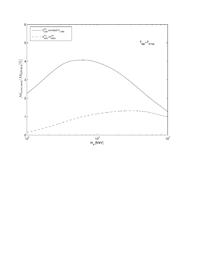
Figure 3.7: Importance of the stretched boxes relatively to the DWBA FSI amplitude $\mathcal{M}^{FSI}_{DWBA}$ of Eq. (3.7), as a function of the mass of the scalar particle for the final $NN$ interaction. The $\pi N$ amplitude is contact re-scattering vertex as in Eq. (3.3) (solid line) and the $\chi$PT amplitude as in Eq. (3.4) (dashed line). The energy is taken at the pion production threshold. Absolute values of the amplitudes are considered.

It is interesting to compare this result with the one of Ref. [82]. As shown in Fig. 3.7, the stretched boxes amplitude is less than $1\%$, of the total amplitude and therefore is about 6 times more suppressed than in the dynamics of the toy model used in that reference. Replacing the $\pi N$ amplitude from $\chi$PT by a simple contact amplitude, the stretched boxes amplitude becomes slightly more important, but they still do not exceed $4\%$ of the DWBA amplitude (solid line in Fig. 3.7).

In terms of the cross section, the weight of the stretched boxes relatively to DWBA is even smaller, of the order of $0.02\%$ at most. This is seen in Fig. 3.8 where we compare, for three different values of the laboratory energy, the cross section obtained with only the DWBA contribution ($\sigma_{DWBA}$), with the one obtained with only the stretched boxes terms ($\sigma_{stretched}$). In both cases considered, $V_{\pi NN}^{PV}+V_{\pi\pi NN}^{\chi Pt}$ and $V_{\pi NN}^{PV}$ + contact (left and right panel in Fig. 3.8, respectively) the cross section with the DWBA terms is clearly dominant, and in a more pronounced way when compared to the less realistic case of Ref. [82], not only at threshold but even for higher energies as $440\mathrm{MeV}$.

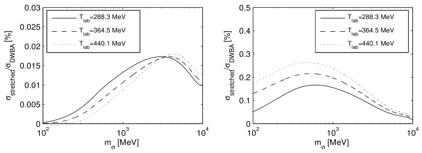
Figure 3.8: Importance of the stretched boxes compared to the DWBA (FSI) for the cross section as a function of the mass of the scalar particle for the final $NN$ interaction. The $\pi N$ amplitude is the $\chi$PT amplitude (left) and a contact re-scattering vertex (right).

However, we note that the ratios and energy dependence of the amplitudes and of the cross sections are significantly influenced by the $\pi N$ amplitude used in the calculation. The stretched boxes are seen to be amplified by the contact $\pi N$ re-scattering amplitude, due to an interplay between the $\pi N$ and the $NN$ amplitudes. Relatively to the more realistic $\chi$Pt amplitude, the contact $\pi N$ amplitude gives a larger weight to the low-momentum transfer. The realistic $\pi N$ amplitude satisfies chiral symmetry. This implies cutting small momenta and giving more weight to the region of large momentum transfer, which however in turn is cut by the nucleonic interactions. The difference between the two $\pi N$ amplitudes is clearly seen by comparing the behaviour of each curve on the left panel of Fig. 3.8 with the corresponding curves on the right panel, for small values of the $NN$ interaction cut-off.

In the case of the initial-state amplitude, the stretched boxes amplitude is also much smaller than the DWBA amplitude for the two cases shown in Fig. 3.9.

The cross sections obtained with only the stretched boxes terms were found to be less than $1.2\%$ of the DWBA cross sections, even for laboratory energies as high as $T_{lab}\sim 440\mathrm{MeV}$ (see Fig. 3.10).

The results presented in Fig. 3.7 to Fig. 3.10 justify the DWBA treatment for pion production.

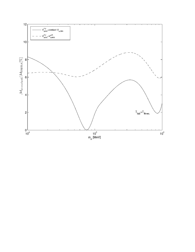
Figure 3.9: The same as Fig. 3.7 but for the DWBA ISI amplitude $\mathcal{M}^{ISI}_{DWBA}$ of Eq. (3.15).

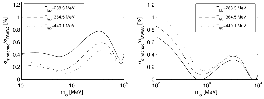
Figure 3.10: The same as Fig. 3.8 but for the ISI case.

3.3 The logarithmic singularity in the pion propagator (ISI)

From the evaluation of the effective pion propagator for the ISI case of Eq. (3.19), at threshold,

$$G_{\pi}^{th.}=\frac{1}{\left(\frac{m_{\pi}}{2}\right)^{2}-\left(\frac{m_{\pi}}{2}-\omega_{\pi}\right)^{2}}=\frac{1}{\omega_{\pi}\left(m_{\pi}-\omega_{\pi}\right)},$$ (3.21)

it is straightforward to conclude that $G_{\pi}$ has a pole, since it is energetically allowed for the exchanged pion to be on-mass-shell $\left(\omega_{\pi}=m_{\pi}\right)$. The treatment of the pole leads to a moving singularity which was not considered in the traditional DWBA calculations of Refs. [36, 56, 57, 63, 66, 81]. It requires a careful numerical treatment which was included in our calculations.

This is done by rewriting $G_{\pi}$ of Eq. (3.19) as

$$G_{\pi}=\frac{1}{\alpha_{1}-\alpha_{2}}\left(\frac{1}{\alpha_{1}-\omega_{\pi}}-\frac{1}{\alpha_{2}-\omega_{\pi}}\right),$$ (3.22)

with

$$\alpha_{1} = F_{2}-\omega_{2}$$ (3.23)

$$\alpha_{2} = F_{1}+E_{\pi}-\omega_{1}.$$ (3.24)

With the definitions $F_{1,2}$, $\omega_{1,2}$ and $\omega_{\pi}$ introduced in Sec. 3.1 (see Appendix B), then Eq. (3.22) reads

$$G_{\pi}=\frac{1}{\alpha_{1}-\alpha_{2}}\left[\frac{\alpha_{1}+\omega_{\pi}}{q_{\pi}I_{2}\left(x_{2}\right)}\frac{1}{y_{1}-x_{1}}-\frac{\alpha_{2}+\omega_{\pi}}{q_{\pi}I_{2}\left(x_{2}\right)}\frac{1}{y_{2}-x_{1}}\right].$$ (3.25)

where $I_{2}\left(x_{2}\right)=\left|\overrightarrow{q_{u}}-\overrightarrow{q_{k}}\right|=\sqrt{q_{u}^{2}-2q_{u}q_{k}x_{2}+q_{k}^{2}}$. The angles involved in the partial wave decomposition performed for the amplitudes are $x_{1}=\measuredangle\left(\overrightarrow{q_{u}}-\overrightarrow{q_{k}},\overrightarrow{q_{\pi}}\right)$ and $x_{2}=\measuredangle\left(\overrightarrow{q_{u}},\overrightarrow{q_{k}}\right)$ (see Appendix E). Here, $y_{i}$, roots of the denominator of $G_{\pi}$, are given by:

$$y_{i}=\frac{\alpha_{i}^{2}-\beta^{2}}{q_{\pi}I_{2}\left(x_{2}\right)}\qquad\text{with }\beta^{2}\equiv m_{\pi}^{2}+\frac{q_{\pi}^{2}}{4}+I_{2}\left(x_{2}\right)^{2}\text{ and }i=1,2$$ (3.26)

Once $G_{\pi}$ is written in this form, for the calculation of the partial wave decomposition, we have to deal with its poles at $x_{1}=y_{i}$. We used the subtraction technique (see Appendix F) exposing the three-body logarithmic singularity:

$$\int_{-1}^{1}\frac{f\left(x_{1},x_{2}\right)}{y_{i}-x_{1}+i\varepsilon}P_{L}\left(x_{1}\right)dx_{1} = \mathbf{PV}\int_{-1}^{1}\frac{f\left(x_{1},x_{2}\right)-f\left(y_{i},x_{2}\right)}{y_{i}-x_{1}}P_{L}\left(x_{1}\right)+2f\left(y_{i},x_{2}\right)Q_{L}\left(y_{i}\right)-$$ (3.27)

$$-i\pi P_{L}\left(y_{i}\right)f\left(y_{i},x_{2}\right)$$

where $P_{L}$ and are the Legendre polynomials of order $L$ and $Q_{L}$ are the Legendre functions of the second kind of order $L$[85]. These last functions exhibit logarithmic singularities which are given by the condition $y_{i}=\pm 1$, which are determined analytically. Then, the integral over the moving logarithmic singularities is handled by a variable mesh. When the number of singularities (always between zero and two) is $n_{s}$, the interval of integration is divided into $2n_{s}+1$ regions including as breaking points those given by the found singularities. In each one of the regions we considered a Gaussian mesh.

3.4 Conclusions

In this Chapter we have generalised the work done in Refs. [82, 83] on the study of the DWBA approaches for the irreducible pion re-scattering mechanism of the reaction $pp\rightarrow pp\pi^{0}$. We considered a physical model for nucleons and pions, combining a pseudo-vector coupling for the $\pi NN$ vertex and the $\chi$PT $\pi N$ re-scattering amplitude. We treated the initial and final state distortion exactly, taking into account in the first case the three-body moving singularities in the pion propagator.

Both for the final- and initial-state interaction, our results show that the DWBA formalism is quite adequate at threshold and even at higher energies, since this part of the full amplitude is clearly seen to be dominant over the stretched boxes. This is independent of the model for the $\pi N$ re-scattering amplitude. Nevertheless, relatively to less realistic models, a chirally constrained amplitude reinforces even more the relative importance of the DWBA amplitude in the total amplitude.

The amplitudes given by Eqs.(3.7) and (3.15) obtained as non-relativistic reductions of the corresponding Feynman diagrams for the final- and initial-state interactions, can now be employed to study the commonly used prescriptions for the energy of the exchanged pion, both in the propagator and at the re-scattering vertex. This energy, not fixed in a non-relativistic quantum-mechanical calculation, was fixed by TOPT to be $\omega_{\pi}$, its on-mass-shell energy.

Since in the time-ordered diagrams energy is not conserved at individual vertices, each of the re-scattering diagrams for the initial- and final-state distortion defines a different off-energy shell extension of the pion re-scattering amplitude, as calculated in Sec. 3.1.1 and Sec. 3.1.2. As a consequence, the two operators for FSI and ISI are different, demanding the evaluation of two different matrix elements of such operators between the quantum-mechanical $NN$ wave functions. In the next Chapter, an alternative approach will be presented, where this problem does not arise.

Chapter 4 The S-matrix approach for quantum mechanical calculations

Abstract: The pion re-scattering process is certainly part of the pion production mechanism, but its importance relative to other contributions varies considerably depending on the approximations made in evaluation of the effective operators. In this Chapter, we will re-examine the nature and extent of this uncertainty. The pion re-scattering operator originated from the S-matrix construction, previously applied only below pion production threshold, is seen here to approximate well the exact DWBA result consistent with time-ordered perturbation theory.

4.1 The pion re-scattering operator in the S-matrix technique

To derive the quantum mechanical effective operators for pion production, and other effective nuclear operators in general, one starts from the relativistic (effective) Lagrangian written in terms of hadronic fields. The interactions, mediated by meson exchanges before and after the production reaction takes place, are included in the effective $NN$ (and nucleon-meson) interaction, while from the irreducible parts connected to the reaction mechanism (e.g., pion production) one obtains effective operators, whose expectation values are to be evaluated between the initial and final nucleonic wave functions. One aims to get such effective operators consistent with the realistic description of the $NN$ interaction, which can then be used in studies of the corresponding reactions not only in the simplest (one or two-nucleon) systems, but preferably also in heavier nuclei.

The covariant techniques based on the Bethe-Salpeter equation or its quasipotential re-arrangements are these days practically manageable only below meson production threshold. However, above the threshold the dressings of the single hadron propagators and interaction vertices via the meson loops have to be included explicitly. For this reason the construction of the production operator is so far realised mostly in the Hamiltonian quantum-mechanical framework (usually non-relativistic, or, with leading relativistic effects included perturbatively by means of the decomposition in powers of $p/m$, where $p$ is the typical hadronic momentum and $m$ is the nucleon mass).

The derivation of the nuclear effective operators below the meson production threshold within the Hamiltonian framework – leading to hermitian and energy independent $NN$ and $3N$ potentials, and conserved electromagnetic and partially conserved weak current operators – can be done in many different ways (see discussion in Refs. [86, 87, 88, 89] and references therein). At the non-relativistic order the results are determined uniquely. As for the leading order relativistic contributions, they were shown to be unitarily equivalent[89]. The unitary freedom allows to choose the $NN$ potentials to be static (in the CM frame of the two-nucleon system) and identify them with the successful static semi-phenomenological potentials.

Also, above the threshold energy the static limit is commonly employed, since more elaborate descriptions which include the mesonic retardation and loop effects are technically considerably more complex [90, 91, 92], especially for systems of more than two nucleons. Both the static approaches and the ones including “retardation” typically consider contributions of several one-meson exchanges, and the potentials are fitted to describe the data. It is therefore difficult to assess how well do they approximate the covariant amplitudes (corresponding to the same values of physical masses and coupling constants) which are so far outside the scope of existing calculational schemes, but which we believe do provide in principle the consistent description of the considered reactions.

Thus, the ultimately exact approach to the description of pion production (and in particular of the pion re-scattering contribution) would be either the covariant Bethe-Salpeter or quasipotential frameworks (extended above the pion threshold) or the quantum mechanical coupled-channel technique including retardation. In these approaches one has to treat consistently the non-hermitian energy-dependent $NN$ interaction (fitted to the data also above pion production threshold) and consider besides the effects of renormalisation of vertices, masses and wave functions via meson loops.

In this Chapter (following Refs. [82, 83, 84, 93]) we rather numerically estimate the range of the predictions from several frequently used simplifying approximations, and compare them to the result obtained from the reduction of the corresponding covariant Feynman diagrams for the pion re-scattering operator. This reduction coincides with the time-ordered perturbation theory[84]. To this end we deal with retardation effects in the exchanged pion propagator, i.e., its energy dependence, as well as with the energy dependence of the $\pi$N scattering amplitude in the vertex, from which the produced pion is emitted.

4.1.1 Factorisation of the effective re-scattering operator

In the previous Chapter, we made the connection to the usual representation of the pion re-scattering operator for non-relativistic calculations, following the work of Ref. [84]. We started from the covariant two-nucleon Feynman amplitudes including final and initial state interaction (FSI and ISI, respectively), shown in Fig. 4.1a) and 4.1b)).

Figure 4.1: Feynman diagrams for pion re-scattering. The pion field is represented by a dashed line, the $NN$ interaction by solid double line and the nucleons by solid lines.

To obtain the effective re-scattering operator, the negative energy contributions in the nucleon propagators (to be included in complete calculations) were neglected. By integrating subsequently over the energy of the exchanged pion the resulting Feynman amplitudes were transformed into those following from time-ordered perturbation theory.

The irreducible “stretched box diagrams” (i.e., those with more than one meson in flight in the intermediate states) give a very small contribution and can be therefore also neglected (as we showed in the previous Chapter in Fig. 3.7-Fig. 3.10). Thus, the full covariant amplitude is in the lowest order Born approximation well approximated by the product of the $NN$ potential and the effective pion re-scattering operator, which can be extracted from these time-ordered diagrams (Fig. 4.2).

Figure 4.2: The two time-ordered diagrams for FSI considered here. The additional stretched box diagrams are neglected.

Summarising, what was obtained in Chapter 3, for the final state distortion amplitude, was

$${\mathcal{M}}_{FSI} = \int\frac{d^{3}q^{\prime}}{(2\pi)^{3}}\,V_{\sigma}\,\frac{1}{F_{1}+F_{2}-\omega_{1}-\omega_{2}+i\varepsilon}\,\hat{O}_{rs}$$ (4.1)

$$\hat{O}_{rs} = -\frac{1}{2\omega_{\pi}}\left[\frac{f(\omega_{\pi})}{E_{2}-\omega_{2}-\omega_{\pi}}+\frac{f(-\omega_{\pi})}{E_{1}-\omega_{1}-E_{\pi}-\omega_{\pi}}\right]=\frac{1}{2}\,\tilde{f}\,G_{\pi}.$$ (4.2)

The effective pion re-scattering operator was factorised into an effective pion re-scattering vertex $\tilde{f}$ and an effective pion propagator $G_{\pi}$. For the diagram with FSI (Fig. 4.2) this factorisation reads (Eq. (3.8), Eq. (3.10) and Eq. (3.12)):

$$\tilde{f} = \frac{1}{\omega_{\pi}}\left[(E_{1}-\omega_{1}-E_{\pi}-\omega_{\pi})f(\omega_{\pi})+(E_{2}-\omega_{2}-\omega_{\pi})f(-\omega_{\pi})\right]$$ (4.3)

$$G_{\pi} = -\frac{1}{(E_{1}-\omega_{1}-E_{\pi}-\omega_{\pi})(E_{2}-\omega_{2}-\omega_{\pi})}$$ (4.4)

$$V_{\sigma} = \frac{g_{\sigma}^{2}}{2\omega_{\sigma}}\left[\frac{1}{F_{2}-\omega_{2}-\omega_{\sigma}}+\frac{1}{F_{1}-\omega_{1}-\omega_{\sigma}}\right].$$ (4.5)

As before, $\vec{q}^{\,\prime}$ is the momentum of the exchanged pion, $\omega_{\pi}=\sqrt{m_{\pi}^{2}+\vec{q}^{\,\prime 2}}$ is its on-mass-shell energy and $f(\omega_{\pi})$ is the product of the $\pi N$ amplitude with the $\pi NN$ vertex. The variables $E_{i},\omega_{i},F_{i}$ are the on-mass-shell energies of the i-th nucleon in the initial, intermediate and final state, respectively, $E_{\pi}$ is the energy of the produced pion, $E_{1}+E_{2}=F_{1}+F_{2}+E_{\pi}$.

Again, we note that $f\left(\omega_{\pi}\right)$ in fact depends on the three-momenta and energies of both (the exchanged and the produced) pions and on the nucleon spin. We indicate explicitly only the dependence on the exchanged pion energy, as the only one important for the considerations below.

The inclusion of some pieces of the integrand of Eq. (4.1) into the propagator $G_{\pi}$ and of others in the modified vertex $\tilde{f}$ is somewhat arbitrary. The appearance of the unusual effective propagator $G_{\pi}$ and the effective vertex $\tilde{f}$ is the result of combining two time-ordered diagrams with different energy dependence into a single effective operator.

The $NN$ interaction is in Fig. 4.2 and in Eq. (4.1) simulated by a simple $\sigma$-exchange potential. Though not realistic, this interaction suffices for model studies of approximations employed in derivations of the effective pion re-scattering operator, as done in references Refs. [82, 83]. Since some results do depend on the behaviour of the $NN$ scattering wave function, in particular in the region of higher relative momenta, we perform our calculations (as in Ref. [84]) also with $V_{\sigma}$ replaced by a full $NN$ T-matrix, generated from the realistic Bonn B potential[62].

We note that the meson poles are not neglected in the integration over the energy $Q^{\prime}_{0}$ of the exchanged pion, which generates Eq. (4.1) (see Sec. 3.1). A result similar to Eq. (4.1) can also be obtained for the amplitude with the initial state interaction (ISI).

$${\mathcal{M}}_{ISI} = -\int\frac{d^{3}q^{\prime}}{(2\pi)^{3}}\,V_{\sigma}\,\frac{1}{E_{1}+E_{2}-\omega_{1}-\omega_{2}+i\varepsilon}\,\hat{O}_{rs}$$ (4.6)

$$\hat{O}_{rs} = -\frac{1}{2\omega_{\pi}}\left[\frac{f(\omega_{\pi})}{E_{\pi}+F_{1}-\omega_{1}-\omega_{\pi}}+\frac{f(-\omega_{\pi})}{F_{2}-\omega_{2}-\omega_{\pi}}\right]=\frac{1}{2}\,\tilde{f}\,G_{\pi}$$ (4.7)

$$\tilde{f} = \frac{1}{\omega_{\pi}}\left[(F_{2}-\omega_{2}-\omega_{\pi})f(\omega_{\pi})+(E_{\pi}+F_{1}-\omega_{1}-\omega_{\pi})f(-\omega_{\pi})\right]$$ (4.8)

$$G_{\pi} = -\frac{1}{(E_{\pi}+F_{1}-\omega_{1}-\omega_{\pi})(F_{2}-\omega_{2}-\omega_{\pi})}$$ (4.9)

$$V_{\sigma} = \frac{g_{\sigma}^{2}}{2\omega_{\sigma}}\left[\frac{1}{E_{2}-\omega_{2}-\omega_{\sigma}}+\frac{1}{E_{1}-\omega_{1}-\omega_{\sigma}}\right].$$ (4.10)

The two amplitudes differ however in the contribution from the pion poles to the remaining integration over the three-momentum. For the amplitude with FSI there are no such poles. However, for the ISI case there are values of the exchanged pion three-momentum for which the propagator $G_{\pi}$ has poles. These poles have been considered in all our numerical calculations for the cross section (see Sec. 3.3). As we will see in this Chapter, they are one of the main reasons for deviations between several approximations and the reference results calculated from Eqs. (4.1-4.5) and Eqs. (4.6-4.10) .

It is worth mentioning that although the FSI and ISI diagrams graphically separate the $NN$ interaction and the pion re-scattering part (when the stretched boxes are neglected), they do not define a single effective operator (as a function of nucleon three-momenta and the energy of emitted pion). Since in these time-ordered diagrams energy is not conserved at individual vertices, each of these diagrams defines a different off-energy shell extension of the pion re-scattering amplitude. This is an unpleasant feature, since one would have to make an analogous construction for diagrams with both FSI and ISI. Moreover, one would have to repeat the whole analysis for systems of more than two nucleons. Only after the on-shell approximation is made consistently (in the next subsection), the pion re-scattering parts of FSI and ISI diagrams coincide and one can identify them with a single effective re-scattering operator.

4.1.2 The S-matrix technique

The S-matrix technique is a simple prescription to derive effective nuclear operators from the corresponding covariant Feynman diagrams [86, 87, 88, 89]. For electromagnetic operators and also for $NN$ and $3N$ potentials at energies below the first nucleonic inelasticities, the S-matrix approach analytically reproduces the results of more laborious constructions, based on time-ordered or non-relativistic diagram techniques. We will prove here that the same is numerically true for energies above pion production threshold.

This approach is well defined and understood below the meson production threshold. As a simple tool it was employed also above the threshold in Refs. [47, 57], but only to derive the Z-diagram operators. The two-nucleon effective operators are by definition identified with the diagrams describing the irreducible mechanism of the corresponding reaction. The only exception are the nucleon Born diagrams from which the iteration of the one-nucleon operator has to be subtracted. The operators of the nuclear electromagnetic and weak currents, as well as the pion absorption operators and nuclear potentials, are obtained by a straightforward non-relativistic reduction of the corresponding Feynman diagrams, in which the intermediate particles are off-mass-shell but energy is conserved at each vertex: therefore the derived effective operators are also defined on-energy-shell. The nuclear currents and other transition operators are defined to be consistent with a hermitian energy independent $NN$ potential, which has the usual one boson exchange form employed in realistic models of the $NN$ interaction, and can be used also in systems of more than two nucleons.

The $\sigma$-exchange potential

For the $\sigma$-exchange potential the S-matrix technique in the lowest order of non-relativistic reduction yields

$$V_{\sigma}^{S}=g_{\sigma}^{2}\frac{1}{\Delta^{2}-\left(m_{\sigma}^{2}+\vec{q}_{\sigma}^{\,2}\right)},$$ (4.11)

where $\Delta=\Delta_{1}=\Delta_{2}$, $\Delta_{1}=\epsilon^{\prime}_{1}-\epsilon_{1}$ and $\Delta_{2}=\epsilon_{2}-\epsilon^{\prime}_{2}$, with $\epsilon^{\prime}_{i}$ and $\epsilon_{i}$ being the on-mass-shell energies of the i-th nucleon after and before the meson exchange, respectively. As pointed out above, this defines the potential only on-energy-shell (where actually $\Delta=0$). However, the Lippmann-Schwinger equation and even the first order Born approximation to the wave function require the potential off-energy-shell.

The S-matrix prescription takes the symmetric combination

$$\Delta=\frac{\epsilon^{\prime}_{1}-\epsilon_{1}}{2}+\frac{\epsilon_{2}-\epsilon^{\prime}_{2}}{2}=\frac{\Delta_{1}+\Delta_{2}}{2}.$$ (4.12)

Most realistic $NN$ potentials, namely those fitted to the data below pion threshold, in particular the Bonn B[62] potential used in this work, are energy-independent and static in the nucleon CM frame and are therefore consistent with this construction. The extended S-matrix approach [86, 87, 88, 89] given by Eq. (4.11) defines the most general off-energy-shell continuation of $V_{\sigma}$ as a class of unitarily equivalent potentials parameterised by the “retardation parameter” $\nu$.

We show in Fig. 4.3 the comparison of the cross section for $pp\rightarrow pp\pi^{0}$ with the approximation of Eq. (4.11) and the static approximation ($\Delta=0$) for the potential, to the “exact” reference result of Eq. (4.1) and Eq. (4.6).

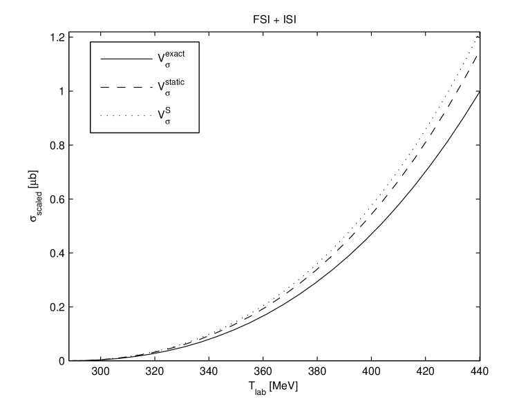
Figure 4.3: Comparison of the cross section for $pp\rightarrow pp\pi^{0}$ calculated with the static and on-shell approximations for the $\sigma$-exchange potential (dashed and dotted lines, respectively) to the reference result of Eq. (4.1) and Eq. (4.6) (solid line), as a function of the laboratory energy $T_{lab}$. The values of the cross sections are scaled by requiring a reference result of $1$ for $T_{lab}=440\mathrm{MeV}$.

From Fig. 4.3, one concludes that the effect of the approximations for $V_{\sigma}$ is small till $Q\approx 0.1m_{\pi}$. As expected, the deviations of the described approximations (dashed and dotted line, respectively) from the reference result (solid line) increase with energy, with a maximum deviation of about $20\%$.

The pion re-scattering operator

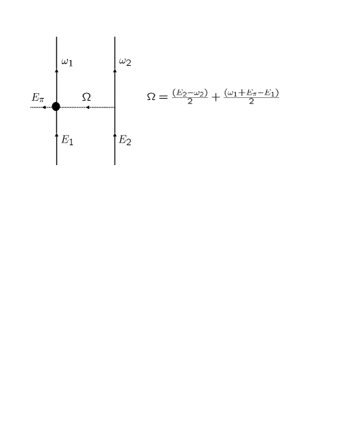
Figure 4.4: Illustration of the S-matrix prescription.

For the pion re-scattering diagram in the FSI case (Eq. (4.2)), according to the S-matrix approach one assumes energy conservation at each vertex. Then the exchanged pion is no longer on-mass-shell and we have to replace $f(\omega_{\pi})\rightarrow f(E_{2}-\omega_{2})$ and $f(-\omega_{\pi})\rightarrow f(E_{2}-\omega_{2})$: in the first time-ordered diagram the virtual pion is entering the re-scattering vertex and in the second one it is emitted from this vertex (as defined on Fig. 4.2). Therefore, one obtains

$$\hat{O}_{rs}\rightarrow\hat{O}_{rs}^{S}=\frac{f\left(E_{2}-\omega_{2}\right)}{\left(E_{2}-\omega_{2}\right)^{2}-\omega_{\pi}^{2}},$$ (4.13)

which is of the S-matrix form[93]. The nucleon energies before and after pion emission are $E_{2}$ and $\omega_{2}$, respectively (see Fig. 4.4).

For three-momentum values corresponding to the on-mass-shell conditions of the nucleons and the emitted pion, the characterisation (4.13) of the S-matrix technique suffices. However, whenever the operators are used in convolution integrals for the nucleon states distortion, the momentum variable is free. The on-mass shell condition has then to be reinforced explicitly by demanding the conservation of energy $\omega_{\pi}=E_{2}-\omega_{2}=-\left(E_{1}-\omega_{1}-E_{\pi}\right)$. This is implemented by setting additionally

$$\Omega=\frac{\left(E_{2}-\omega_{2}\right)}{2}+\frac{\left(\omega_{1}+E_{\pi}-E_{1}\right)}{2},$$ (4.14)

as it is illustrated on Fig. 4.4. The general form of the S-matrix prescription[93] for the pion re-scattering operator becomes henceforth

$$\hat{O}_{rs}^{S}=\frac{f(\Omega)}{\Omega^{2}-\left(m_{\pi}^{2}+\vec{q}^{\,\prime 2}\right)}.$$ (4.15)

Note that the S-matrix approach defines a single effective operator (4.15) both for the FSI and ISI diagrams. In Eq. (4.15), the energy of the exchanged pion is determined by applying consistently energy conservation in both vertices of each diagram and guaranteeing that intermediate particles are on-mass shell. The prescription (4.14) is also consistent with the most realistic $NN$ potentials (see Eq. (4.12)).

4.2 Energy prescriptions for the exchanged pion

The on-shell approximation (also labelled the “$E-E^{\prime}$” approximation[82]) as introduced in Refs. [80, 82, 83] actually coincides with the approximation defined by Eq. (4.13). The re-scattering operator of Eq. (4.13) can indeed be obtained directly from Eq. (4.3) and Eq. (4.4) by the substitutions following from the on-energy-shell prescription and the energy conservation in individual vertices $\Omega=E_{2}-\omega_{2}=-\left(E_{1}-\omega_{1}-E_{\pi}\right)$ as follows:

$$\hat{O}_{rs}\rightarrow-\frac{1}{2\left(E_{2}-\omega_{2}\right)}\frac{-2\left(E_{2}-\omega_{2}\right)\times f\left(E_{2}-\omega_{2}\right)+0\times f\left(\omega_{2}-E_{2}\right)}{\left(E_{2}-\omega_{2}-\omega_{\pi}\right)\left(\omega_{2}-E_{2}-\omega_{\pi}\right)}=\hat{O}_{rs}^{on}\,.$$ (4.16)

We note that this form of $\hat{O}_{rs}$ only coincides with Eq. (4.15) for on-mass shell nucleons, which is not the case in intermediate states, where the momentum integration variable does not in general satisfy the condition of Eq. (4.14).

In the work of Ref. [84] the extra kinematic factors in Eq. (4.3) multiplying the function $f\left(\omega_{\pi}\right)$ were interpreted as form factors and kept unaltered, i.e., the substitution $f(\omega_{\pi})\rightarrow f(E_{2}-\omega_{2}),f(-\omega_{\pi})\rightarrow f(E_{2}-\omega_{2})$ was made only in $G_{\pi}$ and $f(\omega_{\pi})$ of Eq. (4.2), not in the kinematic factors included in the function $\tilde{f}$.

In the following we will analyse in detail the S-matrix approach as well as the effects of other approximations frequently used for the energy of the exchanged pion, namely the on-shell, fixed threshold-kinematics and static approximations. The fixed kinematics approximation, besides considering on-mass-shell particles and energy conservation at the vertices, further assumes that the energy of the emitted pion is $m_{\pi}$, its threshold value ($\Omega\rightarrow m_{\pi}/2$ in Eq. (4.15)). On the other hand, the static approximation assumes that no energy is exchanged ($\Omega\rightarrow 0$ in Eq. (4.15)).

Table 4.1 lists the different approximations considered here and in other works for the full re-scattering operator. The corresponding approximations for the pion propagator $G_{\pi}$ and the re-scattering vertex $\tilde{f}$ are in Table 4.2 and Table 4.3, respectively.

$\hat{O}_{rs}$	FSI	ISI
TOPT	$-\frac{1}{2\omega_{\pi}}\left[\frac{f\left(\omega_{\pi}\right)}{E_{2}-\omega_{2}-\omega_{\pi}}+\frac{f\left(-\omega_{\pi}\right)}{E_{1}-\omega_{1}-E_{\pi}-\omega_{\pi}}\right]$	$-\frac{1}{2\omega_{\pi}}\left[\frac{f\left(\omega_{\pi}\right)}{F_{2}-\omega_{2}-\omega_{\pi}}+\frac{f\left(-\omega_{\pi}\right)}{F_{1}+E_{\pi}-\omega_{1}-\omega_{\pi}}\right]$
on-shell	$\frac{f\left(E_{2}-\omega_{2}\right)}{\left(E_{2}-\omega_{2}\right)^{2}-\omega_{\pi}^{2}}$	$\frac{f\left(\omega_{2}-F_{2}\right)}{\left(\omega_{2}-F_{2}\right)^{2}-\omega_{\pi}^{2}}$
fixed-kin.	$\frac{f\left(\frac{m_{\pi}}{2}\right)}{\left(\frac{m_{\pi}}{2}\right)^{2}-\omega_{\pi}^{2}}$	$\frac{f\left(\frac{m_{\pi}}{2}\right)}{\left(\frac{m_{\pi}}{2}\right)^{2}-\omega_{\pi}^{2}}$
static	$-\frac{f\left(0\right)}{\omega_{\pi}^{2}}$	$-\frac{f\left(0\right)}{\omega_{\pi}^{2}}$
S-matrix	$\dfrac{f\left(\frac{\left(E_{2}-\omega_{2}\right)+\left(\omega_{1}+E_{\pi}-E_{1}\right)}{2}\right)}{\left[\frac{\left(E_{2}-\omega_{2}\right)+\left(\omega_{1}+E_{\pi}-E_{1}\right)}{2}\right]^{2}-\omega_{\pi}^{2}}$	$\dfrac{f\left(\frac{\left(\omega_{2}-F_{2}\right)+\left(F_{1}+E_{\pi}-\omega_{1}\right)}{2}\right)}{\left[\frac{\left(\omega_{1}-E_{\pi}-F_{1}\right)+\left(F_{2}-\omega_{2}\right)}{2}\right]^{2}-\omega_{\pi}^{2}}$

Table 4.1: Energy prescriptions for the exchanged pion in the full re-scattering operator. The first line is the reference result coming from TOPT of Eq. (4.2) and Eq. (4.7). The second, third and fourth lines are for the frequently used prescriptions for the energy of the exchanged pion (on-shell[57, 80, 82, 83], fixed-kinematics[36, 55, 56, 63] and static approximation, respectively). The last line presents the explicit expressions for the full production operator in the S-matrix approach of Eq. (4.15).
Note that the S-matrix approach defines a single effective operator: although they may look different because the labels for the energies in the FSI and ISI cases are different, the operators in the last line have the same dependence on the on-shell energies.

$G_{\pi}$	FSI	ISI
TOPT	$\dfrac{1}{\left(\omega_{1}+E_{\pi}-E_{1}+\omega_{\pi}\right)\left(E_{2}-\omega_{2}-\omega_{\pi}\right)}$	$\dfrac{1}{\left(\omega_{1}-E_{\pi}-F_{1}+\omega_{\pi}\right)\left(F_{2}-\omega_{2}-\omega_{\pi}\right)}$
on-shell	$\dfrac{1}{\left(E_{2}-\omega_{2}\right)^{2}-\omega_{\pi}^{2}}$	$\frac{1}{\left(\omega_{2}-F_{2}\right)^{2}-\omega_{\pi}^{2}}$
fixed-kin.	$\dfrac{1}{\left(\frac{m_{\pi}}{2}\right)^{2}-\omega_{\pi}^{2}}$	$\dfrac{1}{\left(\frac{m_{\pi}}{2}\right)^{2}-\omega_{\pi}^{2}}$
static	$-\dfrac{1}{\omega_{\pi}^{2}}$	$-\dfrac{1}{\omega_{\pi}^{2}}$
S-matrix	$\dfrac{1}{\left[\frac{\left(E_{2}-\omega_{2}\right)+\left(\omega_{1}+E_{\pi}+E_{1}\right)}{2}\right]^{2}-\omega_{\pi}^{2}}$	$\dfrac{1}{\left[\frac{\left(\omega_{1}-E_{\pi}-F_{1}\right)+\left(F_{2}-\omega_{2}\right)}{2}\right]^{2}-\omega_{\pi}^{2}}$

Table 4.2: Frequently used prescriptions (on-shell[57, 80, 82, 83], fixed-kinematics[36, 55, 56, 63] and static approximation) for the energy of the exchanged pion in the pion propagator. The first line is the reference result coming from TOPT of Eq. (4.4) and Eq. (4.9). The last line presents the explicit expressions for $G_{\pi}$ within the S-matrix approach.

$\tilde{f}\left(\omega_{\pi}\right)$	FSI	ISI
TOPT	$f\left(\omega_{\pi}\right)f_{1}^{f}+f\left(-\omega_{\pi}\right)f_{2}^{f}$	$f\left(\omega_{\pi}\right)f_{1}^{i}+f\left(-\omega_{\pi}\right)f_{2}^{i}$
on-shell	$f\left(E_{2}-\omega_{2}\right)f_{1}^{f}+f\left(\omega_{2}-E_{2}\right)f_{2}^{f}$	$f\left(\omega_{2}-F_{2}\right)f_{1}^{i}+f\left(F_{2}-\omega_{2}\right)f_{2}^{i}$
fixed-kin.	$f\left(\frac{m_{\pi}}{2}\right)f_{1}^{f}+f\left(-\frac{m_{\pi}}{2}\right)f_{2}^{f}$	$f\left(\frac{m_{\pi}}{2}\right)f_{1}^{i}+f\left(-\frac{m_{\pi}}{2}\right)f_{2}^{i}$
static	$f\left(0\right)f_{1}^{f}+f\left(0\right)f_{2}^{f}$	$f\left(0\right)f_{1}^{i}+f\left(0\right)f_{2}^{i}$

Table 4.3: The same of Table 4.2 but for the re-scattering vertex $\tilde{f}$ alone. The first line is the reference result of Eq. (4.3) and Eq. (4.8). The functions $f^{f}_{k}$ and $f^{i}_{k}$ $\left(k=1,2\right)$ refer to the multiplicative factors mentioned in Sec. 3.1.

As in Chapter 3, for numerical calculations we considered the $NN\rightarrow(NN)\pi$ transition in partial waves ${}^{3}P_{0}\rightarrow(^{1}S_{0})s$ for the $pp\rightarrow pp\pi^{0}$ reaction. The amplitudes and cross sections are evaluated both with the simple interaction $V_{\sigma}$ of Eq. (4.5) and Eq. (4.10) and with the Bonn B potential[62].

We tested the S-matrix prescription for the re-scattering operator (4.15) and the approximations discussed in the previous section (see Table 4.1). We include also the results for the on-shell, fixed threshold-kinematics, static and the S-matrix approximations for the effective pion propagator $G_{\pi}$, as listed in Table 4.2.

In Fig. 4.5 we show that the amplitudes with the S-matrix operator $O^{S}$ (dotted line with +’s on the upper panels) are the closest to the reference result (solid line). Using the same approach both for the operator and for $V_{\sigma}$ increases slightly the gap from the reference result (line with x’s versus solid line on the upper left panel). The fixed threshold-kinematics version of $\hat{O}_{rs}$, denoted as $\hat{O}^{fk}$, works well for small values of the excess energy $Q$, but starts to deviate rapidly with increasing $Q$ (dashed-dotted line in the upper panels of Fig. 4.5). The on-shell approximation for the operator (dotted-line in the upper panels), although deviates largely from the reference result when the $NN$ interaction is described through $\sigma$-exchange, is close to the reference result for the Bonn B potential (right panel). The static approximation for the re-scattering operator ($\hat{O}^{st}$) overestimates significantly the amplitude (dashed versus solid lines in the upper panels). The same conclusions hold individually for the FSI and ISI amplitudes (Fig. 4.6 and Fig. 4.7, respectively).

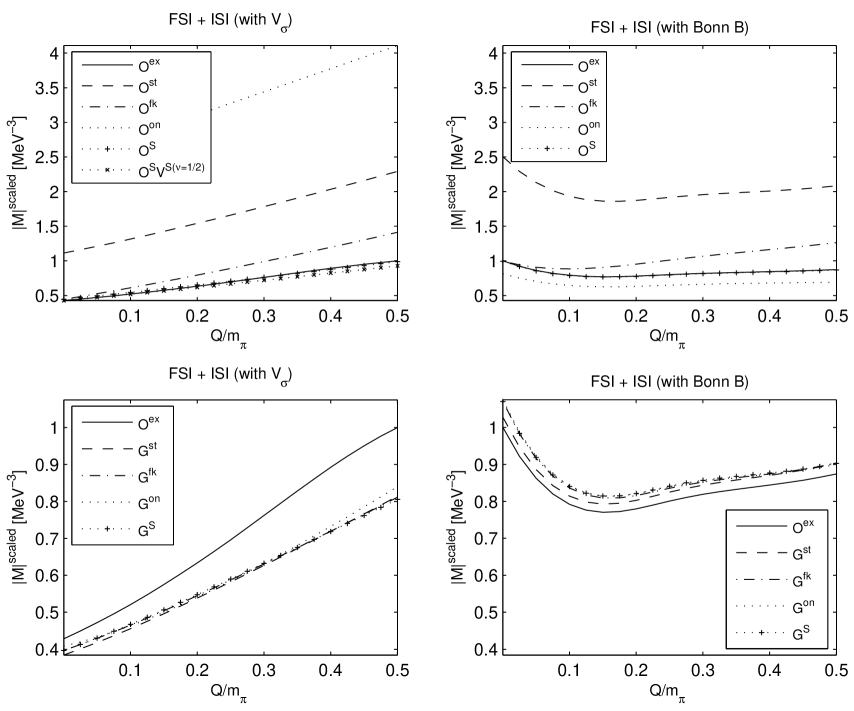
Figure 4.5: Absolute values of the FSI + ISI amplitude as a function of the excess energy $Q=2E-2M-E_{\pi}$ (in units of $m_{\pi}$). The right(left) panels correspond to the amplitudes with $\sigma$-exchange(Bonn B potential) for the $NN$ interaction. The amplitudes are taken at the maximum pion momentum $q_{\pi}^{max}$, determined by $Q$. The upper panels correspond to approximations for the whole operator $\hat{O}_{rs}$; the lower panels to approximations for the pion propagator $G_{\pi}$ only. The solid line $(O^{ex})$ is the reference calculation. The dashed, dashed-dotted, dotted lines and dotted-line with +’s correspond to the static, fixed threshold-kinematics and on-shell approximations and the S-matrix approach, respectively. The corresponding operators are $O^{st}$, $O^{fk}$, $O^{on}$ and $O^{S}$, and $G^{st}$, $G^{fk}$, $G^{on}$ and $G^{S}$. The dotted line with x’s corresponds to both the pion production operator and $\sigma$-exchange potential in the S-matrix approach. All amplitudes were normalised by a factor defined by the maximum value of the reference result.

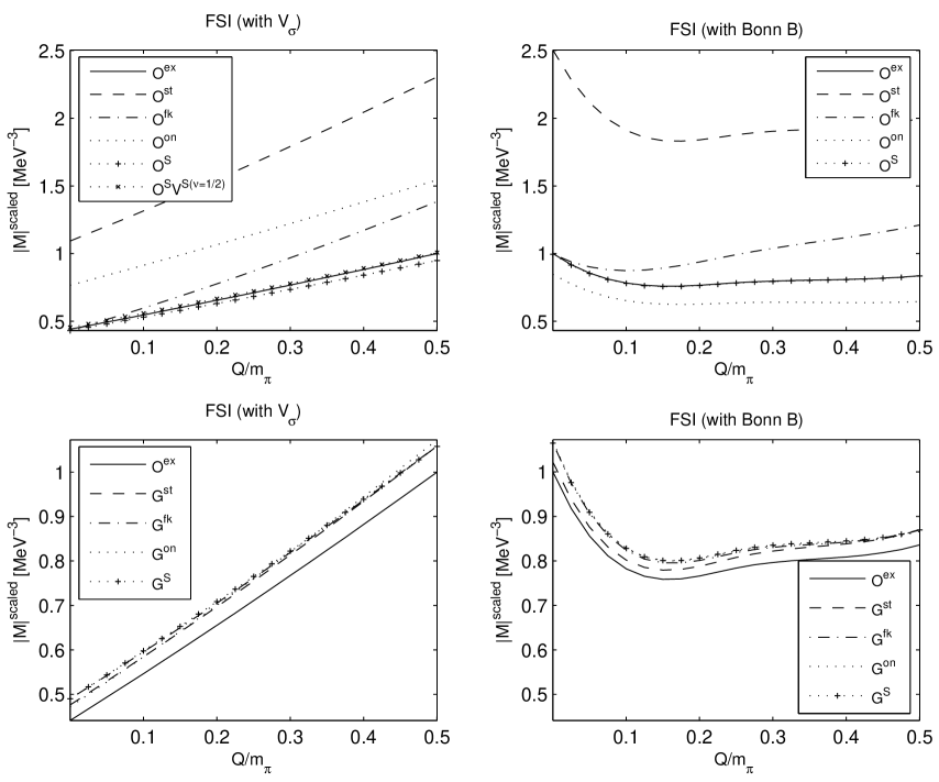
Figure 4.6: The same of Fig. 4.5 but for the FSI amplitude.

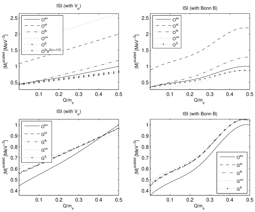
Figure 4.7: The same of Fig. 4.5 but for the ISI amplitude.

The investigation of how much of these features survive below pion production threshold is on Fig. 4.8. The fixed kinematics approximation (dashed-dotted line) is now found to disagree the most with the reference result. The deviation of the static approximation (dashed line) from the reference result (solid line) is much smaller when compared to the situation above threshold of Fig. 4.5. This justifies the traditional approximation of static exchange below threshold. As before, the several approximations for the pion propagator yield results very close to each other (lower panels of Fig. 4.8). Also, the S-matrix approach (dotted line with +’s in the upper panels) describes quite satisfactorily the reference amplitude.

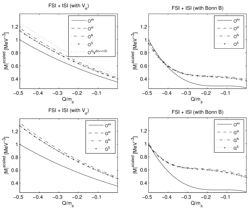
Figure 4.8: Absolute values of the FSI + ISI amplitude as a function of the symmetric of excess energy $Q$ (in units of $m_{\pi}$), below pion production threshold. The meaning of the lines is the same of Fig. 4.5.

4.2.1 Expansion of the effective pion propagator

The lower panels on Fig. 4.5 show that all considered approximations taken only for the effective pion propagator do not differ much from each other, as already found on Ref. [84]. It means that the choices for the energy of the exchanged pion in the effective propagator alone are not very decisive (solid line versus dotted, dashed, dashed-dotted and dotted line with x’s). We notice however that for $\sigma$-exchange there is a considerable deviation of all these approximations from the reference result.

In order to understand this we considered the expansion of the effective pion propagator $G_{\pi}$ in Eq. $\left(\ref{gpi}\right)$ in terms of an “off-mass-shell” dimensionless parameter $y$:

$$y=-\frac{2E-E_{\pi}-\omega_{1}-\omega_{2}}{\omega_{1}-\omega_{2}+E_{\pi}}\,,$$ (4.17)

which measures the deviation of the total energy from the energy of the intermediate state with all three particles on-mass-shell[93]. As before, $E=E_{1}=E_{2}$. This Taylor series expansion can give an insight on the small effect of retardation effects in the propagator, and it reads

$${G_{\pi}}=\underbrace{\frac{1}{\left(\frac{E_{\pi}+\omega_{1}-\omega_{2}}{2}\right)^{2}-\omega_{\pi}^{2}}}_{G^{(1)}_{Tay}}\left[1+\frac{\left(-2E+E_{\pi}+\omega_{1}+\omega_{2}\right)}{\left(\frac{E_{\pi}+\omega_{1}-\omega_{2}}{2}\right)^{2}-\omega_{\pi}^{2}}+...\right]$$ (4.18)

where $G^{(1)}_{Tay}$ has the form of the usual Klein-Gordon propagator.

We notice here that in the case of the ISI amplitude, the representation of the pion propagator $G_{\pi}$ by its Taylor series, the first term of which is $G^{(1)}_{Tay}$, fails due to the presence of a pole in the propagator.

Figure 4.9 compares the first four terms $G_{Tay}^{(i)}(i=1,...,4)$ of this expansion (dashed, dotted and dashed-dotted line and bullets, respectively) with the full effective propagator in Eq. (4.4) (solid line), as a function of the two-nucleon relative momentum $q_{k}$, for two different values of the excess energy $Q$. The convergence of the series demands at least 4 terms. Besides, as expected, this convergence is momentum-dependent.

We have also compared the first term of this expansion with the already considered on-shell, fixed threshold-kinematics and static approximations for the pion propagator. These results are shown in Fig. 4.10. We realise that all these approximations are very near to the 1st order term of the Taylor series. The corrections arising from higher order terms in the expansion are negligible only for low momentum transfer, more precisely in the range $q_{k}<100\mathrm{MeV}$.

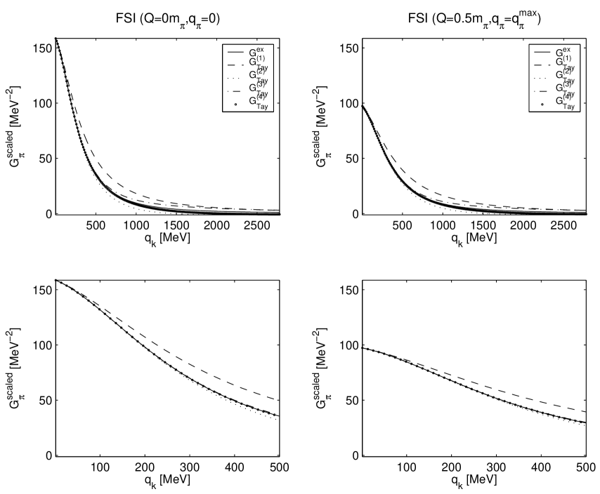
Figure 4.9: Convergence of the Taylor expansion (4.18) of the pion propagator $G_{\pi}$ in the FSI amplitude as a function of the two-nucleon relative momentum. The solid line is the full effective propagator of Eq. (4.4). The dashed, dotted and dashed-dotted lines correspond to the first three terms of the Taylor expansion. The bullets represent the fourth term. Left panel: at threshold; right panel: above threshold at maximum pion momentum for an excess energy $Q=0.5m_{\pi}$. The bottom panels zoom into the region of low relative momentum ($q_{k}<500\mathrm{MeV}$).

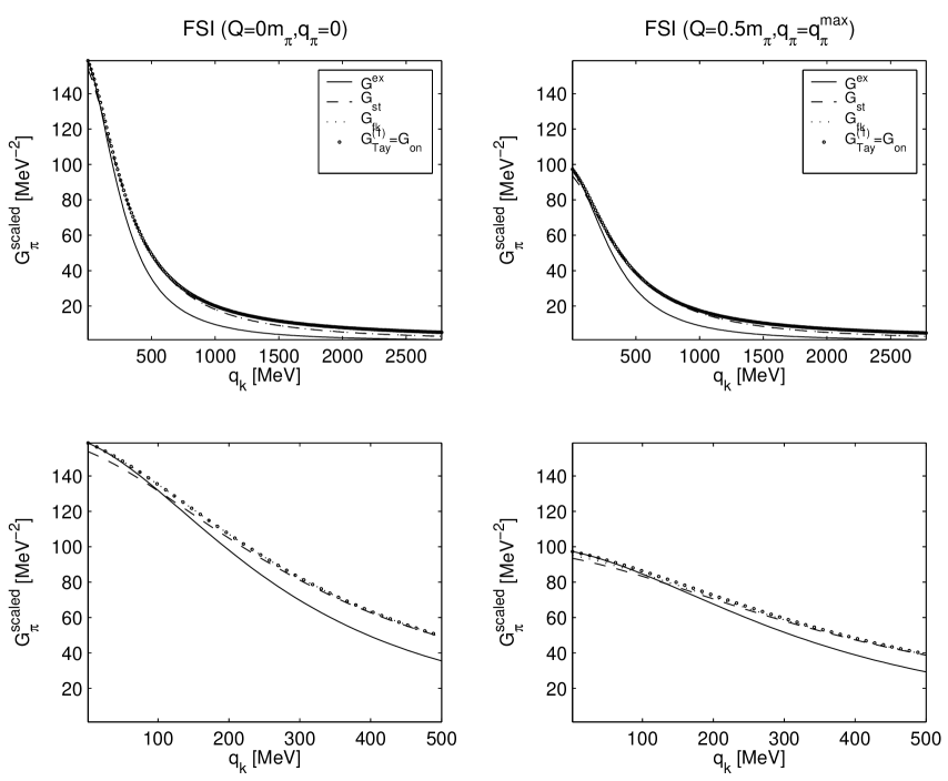
Figure 4.10: Approximations for $G_{\pi}$ in the FSI diagram and the first term of the Taylor series. Left and right panels have the same meaning as on Fig. 4.9.

The deviations of $G^{st}$, $G^{fk}$ and $G^{on}$ from the effective propagator $G_{\pi}$ given by Eq. (4.4) cannot explain the relatively large deviations obtained on the bottom-left panel of Fig. 4.5 between considered approximations and the reference result. These deviations follow from the ISI contribution.

When we compare the results for the final state interaction (lower panels of Fig. 4.6) with the results obtained for the initial state interaction (lower panels of Fig. 4.7), we recognise however that the deviation between the approximate results and the exact one is much more significant for the ISI amplitude. The on-shell $G^{on}$ approximation (and also the fixed kinematics approximation) gives a larger amplitude. Its effect is much more pronounced than it is for the final-state distortion. This difference can be understood since the initial state interaction induces high off-shell energies in the intermediate nucleons. This enlarges the gap between the $G^{on}$ or $G^{fk}$ and the $G^{exact}$ calculations, compared to what happens for the FSI case, where the nucleons emit the outcoming pion before their interaction happens. Also, what is behind the approximations $G^{on}$, $G^{fk}$ or $G^{st}$ being worse representations of the exact amplitude for the ISI case than for the FSI case, is the physics related to the logarithmic singularities of the exact pion propagator. These singularities are present only for the ISI amplitude, but are absent in the case of the approximate forms for that propagator. Their effect is most important for the imaginary part of the amplitude, which is shown in Fig. 4.11.

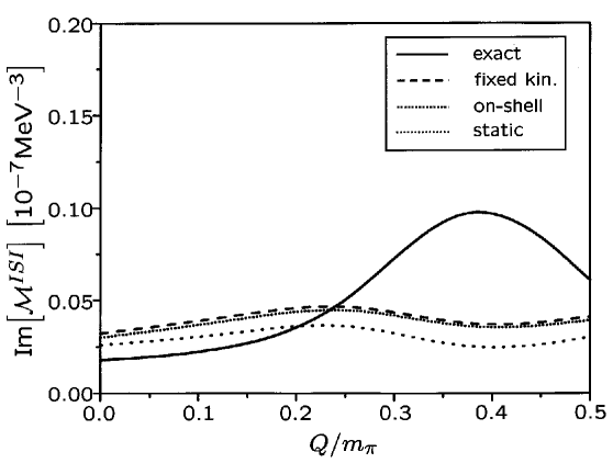
Figure 4.11: Imaginary part of the ISI amplitude $\mathcal{M}_{DWBA}$ of Eq. (4.6) as a function of the excess energy. The exact result (full line) and fixed kinematics (dashed line), on-shell (short-dashed line) and static (dotted line) approximations for the pion propagator are shown.

Also, the weight of the ISI term depends on the $NN$ interaction employed. It is comparable to the FSI term for $V_{\sigma}$ (for which the deviations are large, as seen on the bottom-left panel of Fig. 4.5), but it is less important for the full Bonn B potential (and therefore the corresponding deviations on the bottom-right panel of Fig. 4.5 are indeed much smaller).

All the findings for the amplitudes manifest themselves also in the results for the cross section. We show in Fig. 4.12 the effects of the considered approximations on the cross section, first taking only the FSI contribution. On the left panel the amplitude includes $V_{\sigma}$ for the $NN$ interaction, and on the right panel the Bonn B T-matrix is used. The curves compare the reference result (solid line in all panels) with the S-matrix results (upper panels) and their fixed threshold-kinematics version (lower panels). The S-matrix approach (dashed line) is the closest to the reference result (upper panels of Fig. 4.12).

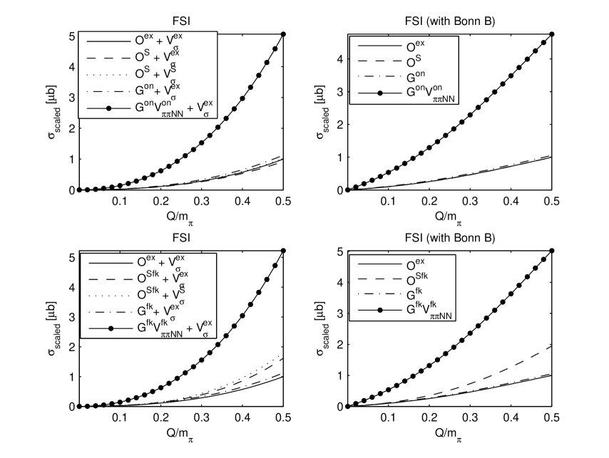
Figure 4.12: Effects of the approximations for the re-scattering operator $\hat{O}_{rs}$ and for the effective pion propagator $G_{\pi}$ as a function of the excess energy $Q$. The cross section curves shown correspond to the FSI amplitude alone. The upper panels correspond to the re-scattering operator $\hat{O}_{rs}$ given by Eq. $\left(\ref{msmat}\right)$ and the lower panels to fixed threshold-kinematics approximation. The solid line is the reference calculation $\left(\ref{afsi}\right)$. The dashed line is the S-matrix calculation for the re-scattering operator $\hat{O}_{rs}$ given by Eq. $\left(\ref{msmat}\right)$ (upper panels) and the fixed threshold-kinematics approximation for $\left(\ref{msmat}\right)$ (lower panels). The dotted line corresponds to take the S-matrix approximation not only for $\hat{O}_{rs}$, but also for the $\sigma$-exchange interaction (4.11). The dashed-doted line corresponds to the on-shell (upper panels) and fixed threshold-kinematics (lower panels) prescriptions only for $G_{\pi}$. The solid lines with bullets refer to the energy prescriptions taken for the propagator $G_{\pi}$ and for $f(\omega_{\pi})$ in Eq. (4.3), as in [84], but not for extra kinematic factors in $\tilde{f}$. All the cross sections were normalised with a factor defined by the maximum value of the reference result.

For the case of the $NN$ interaction described by $V_{\sigma}$ we also show the result following from the S-matrix prescription applied to the $NN$ interaction (dotted line on left panels in Fig. 4.12). For the fixed threshold-kinematics versions (bottom panel) the deviations from the reference result increase pronouncedly with the excess energy $Q$, as expected. The approximations for the energy of the exchanged pion taken in the pion propagator $G_{\pi}$ and in the re-scattering vertex $f(\omega_{\pi})$, but not in the kinematic factors of Eq. (4.3) (see Table 4.3), overestimate the cross section by a factor of 5 (solid line with bullets).

Finally, we present on Fig. 4.13 the comparison between the approximated total cross sections with both FSI and ISI included. The approximation dictated by the S-matrix approach (dashed and dotted lines on the upper panels of Fig. 4.13) is clearly seen as the best one. For the Bonn potential calculation, it practically coincides with the reference result. As shown in the previous section, this procedure amounts to extend the on-shell approximation, used in Ref. [84] for $G_{\pi}$ and $f(\omega_{\pi})$ alone, also to the multiplicative kinematic factors showing up in the operator $\tilde{f}$ (see Eqs. (4.2-4.4)).

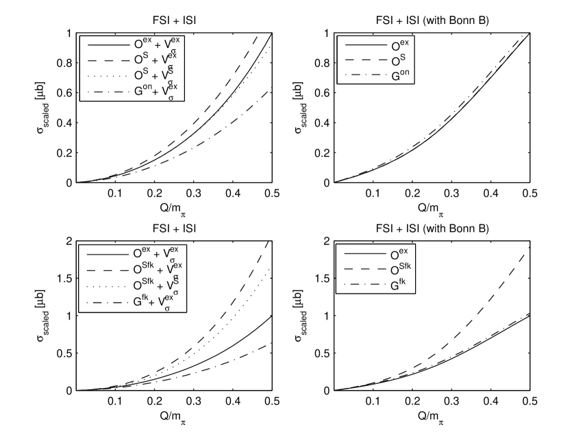
Figure 4.13: The same of Fig. 4.12, but for the total (FSI+ISI) cross-section and considering only the approximations for $\hat{O}$ and $G_{\pi}$.

To conclude we notice, moreover, that for the realistic $NN$ interaction, the difference between the S-matrix approach (upper right panel on Fig. 4.13) and its fixed threshold-kinematics version (lower right panel of the same figure) is not very important near threshold, provided the excess energy does not exceed $\approx 30\mathrm{MeV}$ ($Q/m_{\pi}\sim 0.2$).

4.3 Conclusions

This Chapter discussed the choices for the exchanged pion energy which are unavoidable in the three-dimensional non-relativistic formalism underlying DWBA. The main conclusions are:

1) The usual approximations to the effective pion propagator [36, 56, 63, 80, 84], obtained from a quantum-mechanical reduction of the Feynman diagram describing the pion re-scattering process, are rather close to the first order term of a Taylor series in a parameter measuring off-mass-shell effects in the intermediate states. The series converges rapidly for the FSI amplitude near threshold. As a consequence, retardation effects are not decisive in the pion re-scattering mechanism near the threshold energy for pion production.

2) As for the pion energy in the $\pi N$ re-scattering amplitude, the on-shell approach when used only in $f(\omega_{\pi})$ overestimates significantly the reference result.

3) Nevertheless, and this is the key point of this Chapter, this deviation is dramatically reduced if the approximation coming from the S-matrix approach is used consistently in the whole effective operator[93]. This procedure amounts to extend the on-shell approximation used in Ref. [84] for $G_{\pi}$ and $f(\omega_{\pi})$ to the full operator $\hat{O}_{rs}$, including kinematic factors which differently weight the two dominant time-ordered diagrams. The amplitudes and cross sections obtained with the S-matrix effective operator are very close to those obtained with the time-ordered one in the considered kinematic region. Nevertheless, the static approximation works well below threshold.

The re-scattering operator for the neutral pion production in the isoscalar $\pi$N channel indeed seems to be relatively unimportant: its enhancement reported in previous papers followed from inconsistent or too crude (static or fixed threshold-kinematics) treatment of the energy dependence of the effective operator. Our findings[93] explain why the calculation of Ref. [80], where the on-shell approximation is used, artificially enhances the contribution of the isoscalar re-scattering term. On the other hand, our results indicate that the fixed kinematics choice done in Refs. [36, 55, 56, 63] for the different production operators considered, is valid in the restricted kinematic region where $Q\lesssim 0.2m_{\pi}$.

The re-scattering mechanism is filtered differently by other spin/isospin channels in pion production reactions. For charged pion production reactions the general irreducible re-scattering operator comprises also the dominant isovector Weinberg-Tomozawa term of the $\pi$N amplitude, and its importance is therefore enhanced. Next Chapter investigates these reactions within the S-matrix approach.

Chapter 5 Charged and neutral pion production reactions

Abstract: The S-matrix technique, shown to reproduce the results of time-ordered perturbation theory for the re-scattering mechanism in $\pi^{0}$ production, is applied both to charged and neutral pion production reactions. The contributions from the direct-production, pion re-scattering, Z-diagrams and explicit $\Delta$-isobar excitation terms are considered. High angular momentum partial wave channels are included and the convergence of the partial wave series is investigated.

5.1 Pion production operators

Chapter 4, following the work of Ref. [93], has shown that the S-matrix approach reproduces the energy dependent re-scattering operator for neutral pion production derived from time-ordered diagram techniques. This conclusion provides the motivation to apply this approach further to total cross sections for not only neutral, but also charged pion production. As discussed before, the S-matrix technique has the advantage to define a single effective operator, contrarily to what happens when deriving the quantum-mechanical production operator in the framework of non-relativistic, time-ordered perturbation theory.

Another usual problem of pion production calculations concerns the need of a realistic nucleon-nucleon potential valid for the energies above the pion production threshold, which necessarily are needed for the initial nucleonic states. In this Chapter, we apply for the first time an $NN$ interaction including two boson exchange potentials which describes well not only $NN$ phase-shifts but also inelasticities.

5.1.1 The mechanisms and their operators

We considered the contributions of the impulse, re-scattering, $\Delta$-isobar mechanisms and Z-diagrams as represented in Fig. 5.1.

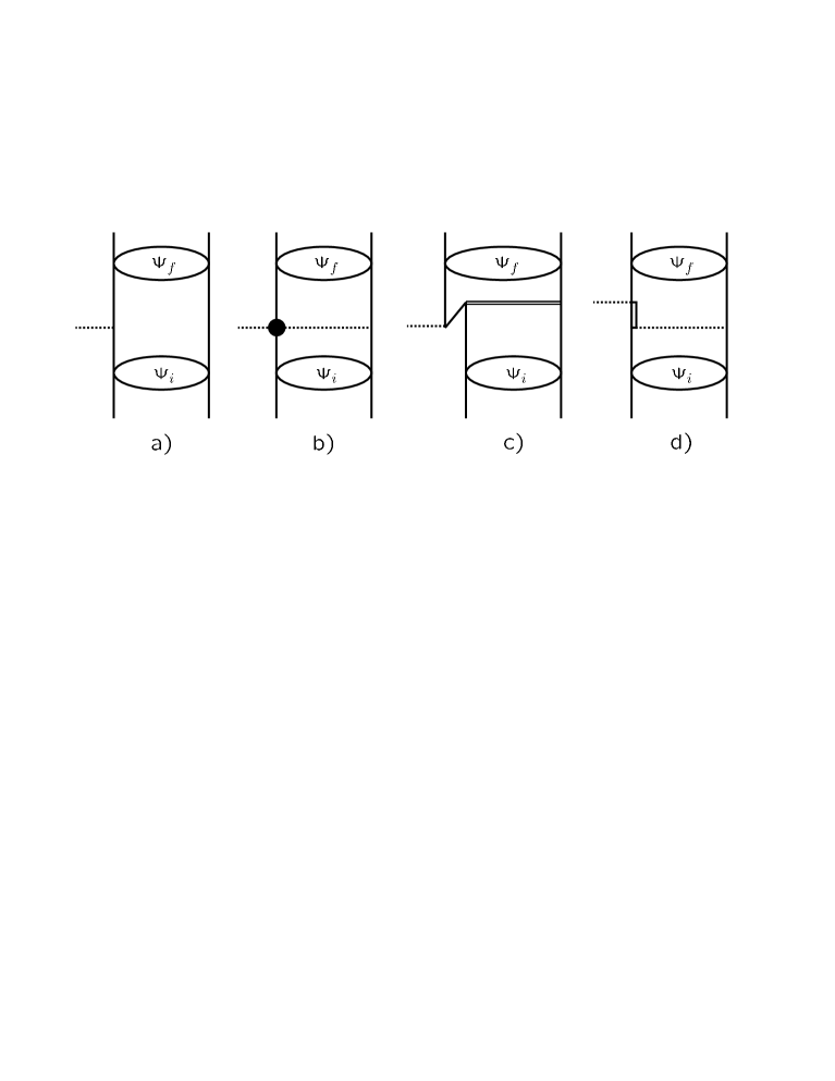
Figure 5.1: Mechanisms considered for charged and neutral pion production. a) direct production, b) re-scattering, c) Z-diagrams and d) $\Delta$-isobar contribution. $T$ is calculated from realistic $NN$ interactions.

The $\pi N$ amplitudes are those of chiral perturbation theory from Ref. [66], resulting from the leading-order Lagrangian of Eq. (2.3) and the next-to-leading order Lagrangian of Eq. (2.3).

From Eq. (2.3) and Eq. (2.3), the single-nucleon emission vertex is

$$\mathcal{M}^{\pi NN}_{a}=\frac{f_{\pi NN}}{m_{\pi}}\tau_{a}^{\left(1\right)}\left[-\left(\vec{\sigma}^{\left(1\right)}\cdot\vec{q}_{\pi}\right)+\frac{E_{\pi}}{2M}\vec{\sigma}^{\left(1\right)}\cdot\left(\vec{p}_{1}+\vec{q}_{1}\right)\right]$$ (5.1)

where $\vec{p}_{1}$ and $\vec{q}_{1}$ are the nucleon momentum before and after pion emission, $\vec{q}_{\pi}$ is the momentum of the emitted pion and $a$ is an isospin index. The second term of Eq. (5.1) accounts for the nucleon recoil effect. For the re-scattering $\pi N$-$\pi N$ vertex (with no isospin flip), one has

$$\mathcal{M}^{\pi\pi NN}_{resc} =-i\frac{m_{\pi}^{2}}{f_{\pi}^{2}}\frac{g_{A}}{f_{\pi}}\left[2c_{1}-\left(c_{2}+c_{3}-\frac{g_{A}^{2}}{8M}\right)\frac{Q^{\prime}_{0}E_{\pi}}{m_{\pi}^{2}}+c_{3}\frac{\vec{q}_{\pi}\cdot\vec{q}^{\,\prime}}{m_{\pi}^{2}}\right]\left[\tau_{a}^{\left(2\right)}\vec{\sigma}^{\left(2\right)}\cdot\vec{q}^{\,\prime}\right]$$

$$-i\frac{1}{f_{\pi}^{2}}\frac{g_{A}}{f_{\pi}}\frac{\delta_{q}}{8}\left[\tau_{3}^{\left(2\right)}\tau_{a}^{\left(1\right)}\vec{\sigma}^{\left(2\right)}\cdot\vec{q}^{\,\prime}+\delta_{3a}\left(\tau^{\left(1\right)}\cdot\tau^{\left(2\right)}\right)\left(\sigma^{\left(2\right)}\cdot\vec{q}^{\,\prime}\right)\right]$$

and for the Weinberg-Tomozawa term,

$$\mathcal{M}^{\pi\pi NN}_{WT}=\frac{g_{A}}{2f_{\pi}}\frac{1}{4f_{\pi}^{2}}\epsilon_{abc}\tau_{b}^{\left(1\right)}\tau_{c}^{\left(2\right)}\left[Q^{\prime}_{0}+E_{\pi}\right]\vec{\sigma}^{\left(1\right)}\cdot\vec{q}^{\,\prime},$$ (5.3)

where $Q^{\prime}_{0}$ is the zeroth component of the exchanged pion four-momentum and $\epsilon_{abc}$ the Levi-Civita tensor (as before, $a$, $b$ and $c$ are isospin indices).

The $\Delta$-isobar contribution was calculated from Eq. (2.3) and reads

$$\mathcal{M}^{\pi N\Delta}=i\frac{g_{A}}{2f_{\pi}}\left(\frac{h_{A}}{2f_{\pi}}\right)^{2}\frac{4}{9}\left[2\tau_{a}^{\left(2\right)}+\tau_{b}^{\left(1\right)}\tau_{c}^{\left(2\right)}\varepsilon^{abc}\right]\left(\vec{q}_{\pi}\cdot\vec{q}^{\,\prime}\right)\vec{\sigma}^{\left(2\right)}\cdot\vec{q}^{\prime}\frac{1}{\Delta-E_{\pi}}\frac{1}{\Omega^{2}-\omega_{\pi}^{2}},$$ (5.4)

where $\Omega$ is given by Eq. (4.14). Since the $\Delta$-resonance is here included explicitly, its contribution needs to be subtracted from the values of the low energy constants $c_{i}$’s of Eq. (5.1.1). This was done taking the heavy baryon limit of Eq. (5.4), giving the contribution $c_{3}^{\Delta}\approx-\frac{h_{A}^{2}}{18m_{\pi}}=-2.78\mathrm{GeV}^{-1}$ which was subtracted from the $-5.29\mathrm{GeV}^{-1}$ value of the $c_{3}$ constant appearing in the $\left(\vec{q}_{\pi}\cdot\vec{q}^{\,\prime}\right)$ term of Eq. (5.1.1).

The heavy-meson mediated $Z$-diagrams contributions given in Ref. [47] and used in Ref. [57] for the $\pi^{0}$ production calculation, were also included:

$$\mathcal{M}_{a}^{Z\_\sigma}=-i\frac{f_{\pi NN}}{m_{\pi}}\frac{V_{S}^{+}\left(k\right)}{M}\frac{E_{\pi}}{2M}\vec{\sigma}^{\left(1\right)}\cdot\left(\vec{p}_{1}+\vec{q}_{1}\right)\tau_{a}^{\left(1\right)}$$ (5.5)

for $\sigma$-exchange, and

$$\mathcal{M}_{a}^{Z\_\omega}=+i\frac{f_{\pi NN}}{m_{\pi}}\frac{E_{\pi}}{2M}\frac{V_{V}^{+}\left(k\right)}{M}\tau_{a}^{\left(1\right)}\vec{\sigma}^{\left(1\right)}\cdot\left[\left(\vec{p}_{2}+\vec{q}_{2}\right)+i\vec{\sigma}^{\left(2\right)}\times\vec{k}\right],$$ (5.6)

for $\omega$ exchange, where $V_{S}^{+}$ and $V_{V}^{+}$ are respectively, the scalar component and isospin independent vector component of the nucleon-nucleon interaction. The i-th nucleon final momentum is $\vec{q}_{i}$ and $\vec{k}=\vec{q}_{2}-\vec{p}_{2}$. The kinematics conventions for the diagrams may be found in Appendix B. Details for the partial wave decomposition of the amplitudes are given in Appendix E.

5.1.2 Nucleon-nucleon potentials at intermediate energies

Since the energies considered for the nucleonic initial state interaction are necessarily above the pion production threshold, we took a recently developed $NN$ interaction fitted to the nucleon-nucleon scattering data[90, 94, 95]. This nucleon-nucleon interaction was developed by the Ohio group as an extension of the Bonn family[62] of realistic nucleon-nucleon potentials well into the intermediate and high energies region.

The free $NN$ T-matrices are obtained from a meson-exchange model including $\Delta$-isobar and N*(1440)/N*(1535) degrees of freedom to account for pion-production above the pion threshold[90, 94, 95]. To properly generate inelasticities, the model incorporates the particle data book nucleon resonances as intermediate excitations within two meson exchanges loops. As an extension of the family of the Bonn potentials, it describes well the $NN$ phase-shifts and inelasticities up to $1$ GeV.

The model is based on the solution of the relativistic Thomson equation. This equation was favoured to time-ordered field theory since it gives a good description of the nucleon inelasticities, without the numerical complexities from the one-pion exchange cut singularities. In time-ordered perturbation theory the last ones are formally unavoidable, but actually, the main contribution to the nucleon singularities arise from the nucleon resonances, and the effect from the one-pion exchange cut is indeed quite small.

The Thomson equation for $NN$ scattering was solved in order to obtain the fit of the $NN$ interaction to both phase-shifts and inelasticities. Table 5.1 lists the parameters employed by the Ohio group $NN$ potential and consistently used in all the calculations in this work. Fig. 5.2 shows the quality of the phase shifts in the relevant energy region for the initial and final nucleonic states.

Meson	$m$ $\left[\text{MeV}\right]$	$\frac{g^{2}}{4\pi}$	$\Lambda$ $\left[\text{MeV}\right]$
$NN\alpha$-vertices
$\pi$	$138.03$	$13.8$	$1519$
$\eta$	$547.30$	$5.81$	$830$
$\omega$	$782.60$	$23.1$	$1382$
$\rho$	$769.00$	$1.09$	$1275$
$a_{0}$	$983.00$	$4.75$	$1004$
$\sigma\left(T=1\right)$	$497$	$5.502$	$1807$
$\sigma\left(T=0\right)$	$482$	$3.513$	$1990$
$\eta^{\prime}$	$958$	$1.62$	$1433$
$f_{0}\left(980\right)$	$980$	$2.50$	$1274$
$N\Delta\alpha$-vertices		$\frac{f^{2}}{4\pi}$
$\pi$	$138.03$	$0.224$	$640$
$\rho$	$769.00$	$20.45$	$1508$

Table 5.1: $NN$-meson and $N\Delta$-meson vertices of the Ohio group $NN$ model. The meson mass is $m$, the coupling constants are $g$ and $f$, and $\Lambda$ is the form-factor cutoff. All of the corresponding form factors are of the monopole type $\left(\frac{\Lambda^{2}-m^{2}}{\Lambda^{2}+k^{2}}\right)$[94].

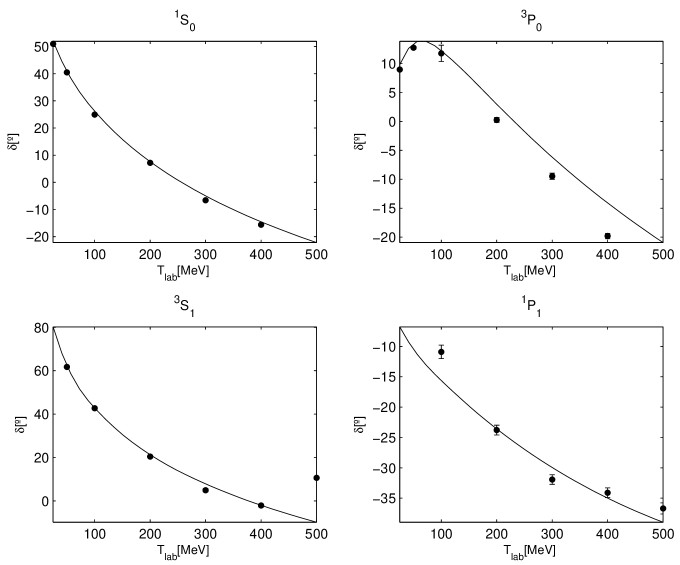
Figure 5.2: Phase shifts calculated with the Ohio group $NN$ potential.

5.2 Calculational details

5.2.1 Three-body kinematics

The phase-space of the reaction $NN\rightarrow B_{1}B_{2}x$ is five-dimensional: the three particles in the final state introduce $3\times 3=9$ degrees of freedom, but the four-momentum conservation reduces this number to $5$. For energies close to threshold, the final state can be treated non-relativistically. The natural coordinate system is therefore given by the Jacobi coordinates[96] where first the relative momentum of one pair of particles is constructed, and then the momentum of the third particle is calculated relatively to the two-body system. Obviously, there are three equivalent sets of variables possible.

For reactions of the type $NN\rightarrow B_{1}B_{2}x$ it is common to work with the relative momentum of the two-nucleon system and to treat the meson $x$ separately, as the spectator particle. This choice is theoretically the most convenient, since one is working already with the relative momentum of the dominant final state interaction. Close to threshold, for the final-state distortion (but not for the initial-state distortion), the nucleons can be treated as non-relativistic, and thus for any given relative energy of the outgoing two-nucleon system,

$$\varepsilon=\frac{q_{k}^{2}}{M}.$$ (5.7)

The modulus of the meson momentum $\left|\vec{q}_{x}\right|$ is fixed by energy conservation. The phase-space is then

$$\xi=\left\{\varepsilon,\Omega_{k},\Omega_{\pi}\right\}$$ (5.8)

where $\Omega_{k}$ and $\Omega_{\pi}$ are the solid angle for the relative $NN$ momentum and for the pion momentum, respectively (see Appendix G). initial state will be denoted by $\vec{p}$. Explicit expressions for the vectors appearing are given in Appendix A. As long as the initial state is unpolarised, the system has azimuthal rotation symmetry, reducing the number of degrees of freedom from $5$ to $4$.

5.2.2 The role of the different isospin channels

Meson production reactions in nucleon-nucleon collisions give also the possibility to manipulate another internal degree of freedom: the isospin. Nucleons are isospin $\frac{1}{2}$ particles in a $\mathcal{SU}\left(2\right)$ doublet,

$$\left|p\right\rangle\equiv\left|t=\frac{1}{2},t_{3}=+\frac{1}{2}\right\rangle\text{ \ and \ }\left|n\right\rangle\equiv\left|t=\frac{1}{2},t_{3}=-\frac{1}{2}\right\rangle,$$ (5.9)

where $\left|p\right\rangle$ and $\left|n\right\rangle$ represent the proton and neutron wave functions, respectively, and $t_{3}$ is the third component of the isospin operator $\mathbf{t}$.

A two-nucleon pair can be either in an isotriplet state (total isospin $T=1$ with the three possible projections of the total isospin $T_{3}=+1$ for a $pp$ state, $T_{3}=0$ for a $pn$ state and $T_{3}=-1$ for a $nn$ state) or in an isosinglet state ($T=0$ with $T_{3}=0$ for a $pn$ state).

Even in an isospin conserving situation, various transitions are possible, depending on whether an isovector or an isoscalar particle is produced. In particular, pion production in $NN$ collisions can be expressed in terms of only three independent reactions with cross sections denoted by $\sigma_{10}$, $\sigma_{01}$ and $\sigma_{11}$ (here, the reference of Ref. [5] is adopted, where $T_{i}$ and $T_{f}$ in $\sigma_{T_{i}T_{f}}$ are the $NN$ pair initial and final total isospin, respectively). Isospin conservation forbids the existence of $\sigma_{00}$. In total, there are seven relations for $NN\rightarrow NN\pi$ reactions[2, 97]:

$$\sigma\left(pp\rightarrow pp\pi^{0}\right) = \sigma_{11}$$ (5.10)

$$\sigma\left(pp\rightarrow pn\pi^{+}\right) = \sigma_{10}+\sigma_{11}$$ (5.11)

$$\sigma\left(np\rightarrow np\pi^{0}\right) = \frac{1}{2}\left[\sigma_{10}+\sigma_{01}\right]$$ (5.12)

$$\sigma\left(np\rightarrow pp\pi^{-}\right) = \frac{1}{2}\left[\sigma_{11}+\sigma_{01}\right]$$ (5.13)

$$\sigma\left(np\rightarrow nn\pi^{+}\right) = \frac{1}{2}\left[\sigma_{11}+\sigma_{01}\right]$$ (5.14)

$$\sigma\left(nn\rightarrow np\pi^{-}\right) = \sigma_{10}+\sigma_{11}$$ (5.15)

$$\sigma\left(nn\rightarrow nn\pi^{0}\right) = \sigma_{11}$$ (5.16)

Note that none of the reactions involves more than two of the fundamental cross sections and that the last two reactions are related with the first two by charge symmetry. The relative strength of the different transition amplitudes can thus provide significant information on the production operator. At medium energies, the cross sections $\sigma_{11}$ and $\sigma_{10}$ are dominated by the excitation of the intermediate $\Delta_{33}$ resonance and are well measured even close to threshold. In contrast, the isoscalar cross section $\sigma_{01}$, which has to be extracted from pion production data in neutron-proton and proton-proton collisions is not well known. Actually, the determination of $\sigma_{01}$ includes a principal model dependence, as

$$\sigma_{np\rightarrow pp\pi^{-}}=\frac{1}{2}\left(\sigma_{11}+\sigma_{01}\right)$$ (5.17)

only holds in the case of exact isospin invariance. However, due to the different particle masses entering in the reactions $np\rightarrow pp\pi^{-}$, $np\rightarrow nn\pi^{+}$ and $pp\rightarrow pp\pi^{0}$, isospin invariance is only an approximate symmetry, and thus the comparison of the cross sections can not be performed at the same beam energy, as mentioned before[33].

Meson production data close to threshold in $np$ collisions suffer from the fact that only relative cross section measurements have been performed, as a consequence of the (poor) quality of the neutron beam. Unfortunately, the isospin cross section $\sigma_{01}$ can only be accessed via these $np$ interactions. It is obtained from the reaction cross section for $np\rightarrow pp\pi^{-}$ by subtracting the $\sigma_{11}$ part, which results in larger uncertainties than in other isospin cross sections.

5.2.3 Partial wave analysis

Some of the complexity inherent to three-body final state reactions can be dealt using partial wave analysis. For energies close to threshold, since the total kinetic energy in the final state is small, the reactions are dominated by transitions to states with low orbital angular momentum values. Therefore, an expansion of the outgoing spherical waves will involve mainly low-order spherical harmonics, and thus the observables should have a relatively simple angular dependence.

The amplitude of the outgoing wave in spin state $\sigma_{1}\sigma_{2}\sigma_{x}$ obtained when the nucleons in the initial state have spin projections $\sigma_{a}$ and $\sigma_{b}$ [98, 99] is given by

$$M_{\sigma_{a}\sigma_{b}}^{\sigma_{1}\sigma_{2}\sigma_{x}} =iK_{i}\sum_{\alpha_{i}\alpha_{f}\alpha_{m}}\sqrt{\frac{2L_{i}+1}{2J+1}}\left\langle s_{a}s_{b}\sigma_{a}\sigma_{b}\left|S_{i}\sigma_{i}\right.\right\rangle\left\langle L_{i}S_{i}0\sigma_{i}\left|JM\right.\right\rangle$$ (5.18)

$$\left\langle s_{1}s_{2}\sigma_{1}\sigma_{2}\left|S_{f}\sigma_{f}\right.\right\rangle\left\langle S_{f}L_{if}\sigma_{f}\lambda_{f}\left|j_{f}m_{f}\right.\right\rangle\left\langle s_{x}l_{x}\sigma_{x}\lambda_{x}\left|j_{x}m_{x}\right.\right\rangle$$

$$\left\langle t_{a}t_{b}\nu_{a}\nu_{b}\left|T_{i}\nu_{i}\right.\right\rangle\left\langle t_{1}t_{2}\nu_{1}\nu_{2}\left|T_{f}\nu_{f}\right.\right\rangle\left\langle T_{f}t_{x}\nu_{f}\nu_{x}\left|T_{i}\nu_{i}\right.\right\rangle$$

$$\left\langle j_{f}j_{x}m_{f}m_{x}\left|JM\right.\right\rangle U_{\alpha_{i}\alpha_{f}}Y_{\lambda_{f}}^{L_{f}}\left(\hat{q}_{k}\right)Y_{\lambda_{x}}^{l_{x}}\left(\hat{q}\right)$$

where $L_{i}$, $S_{i}$ and $J$ are respectively, the two initial nucleon orbital angular momentum, spin and total angular momentum, and $U_{\alpha_{i}\alpha_{f}}$ is a matrix element depending on the quantum numbers in both initial state $\alpha_{i}=\left\{L_{i}\text{, }S_{i}\text{, }J\text{ and }T_{i}\right\}$ and final state $\alpha_{f}=\left\{S_{f}\text{, }L_{f}\text{, }l_{x}\text{, }j_{f}\text{, }j_{x}\text{ and }T_{f}\right\}$. This matrix element is also a function of the energy sharing parameter $\varepsilon$.

The individual nucleon spin quantum numbers are $s_{a}$ and $s_{b}$, with the corresponding magnetic quantum numbers $\sigma_{a}$ and $\sigma_{b}$. In the final state the nucleon spin quantum numbers are represented by $s_{1}$ and $s_{2}$ with spin projections $\sigma_{1}$ and $\sigma_{2}$, and the $NN$ total spin quantum number is $S_{f}$. The $NN$ relative orbital angular momentum is $L_{f}$ and the $NN$ total angular momentum is $j_{f}$.

For the produced meson, the spin is represented by quantum numbers $s_{x}$ and $\sigma_{x}$, the angular momentum relative to the $NN$ centre of mass is $l_{x}$ and the vector sum of $s_{x}$ and $l_{x}$ is $j_{x}$. The isospin quantum numbers are represented by $t$ and $\nu$. $K_{i}$ is a kinematic constant arising from phase-space (as defined in Eq. (G.12)). The sum in $\left(\ref{ms123}\right)$ extends over the initial and final state quantum numbers $\alpha_{1}$ and $\alpha_{2}$, and also the magnetic quantum numbers $\alpha_{m}=\left\{\sigma_{i}\text{, }\sigma_{f}\text{, }M\text{, }m_{f}\text{, }m_{x}\text{, }\lambda_{f}\text{, }\lambda_{x}\text{, }\nu_{i}\text{ and }\nu_{f}\right\}$. These notations are summarised in Table 5.2.

	$N$	Tot${}_{NN_{\text{initial}}}$	$N$	Tot${}_{NN_{\text{final}}}$	$\pi$
Spin	$s_{a}$ and $s_{b}$	$S_{i}$	$s_{1}$ and $s_{2}$	$S_{f}$	$s_{x}$
projection	$\sigma_{a}$ and $\sigma_{b}$	$\sigma_{i}$	$\sigma_{1}$ and $\sigma_{2}$	$\sigma_{f}$	$\sigma_{x}$
Orbital mom.		$L_{i}$		$L_{f}$	$l_{x}$
projection				$\lambda_{f}$	$\lambda_{x}$
Total ang. mom.		$J$		$j_{f}$	$j_{x}$
projection		$M$		$m_{f}$	$m_{x}$
Isospin	$t_{a}$ and $t_{b}$	$T_{i}$	$t_{1}$ and $t_{2}$	$T_{f}$	$t_{x}$
projection	$\nu_{a}$ and $\nu_{b}$	$\nu_{i}$	$\nu_{1}$ and $\nu_{2}$	$\nu_{f}$	$\nu_{x}$

Table 5.2: Summary of the notations for the nucleon and pion spin, orbital momentum, total angular momentum and isospin.

Note that as in the two particle case, the complexity of the angular pattern is determined by the final state orbital angular momentum values $L_{f}$ and $l_{x}$. Since $s_{x}=\sigma_{x}=0\Rightarrow j_{x}=l_{x}$ and $m_{x}=\lambda_{x}$, $\left(\ref{ms123}\right)$ simplifies to

$$M_{\sigma_{a}\sigma_{b}}^{\sigma_{1}\sigma_{2}\sigma_{x}} =iK_{i}I_{\pi}I_{s}\sum_{\alpha_{1}\alpha_{2}\alpha_{m}}\sqrt{\frac{2L_{i}+1}{2J+1}}\left\langle s_{a}s_{b}\sigma_{a}\sigma_{b}\left|S_{i}\sigma_{i}\right.\right\rangle\left\langle L_{i}S_{i}0\sigma_{i}\left|JM\right.\right\rangle$$ (5.19)

$$\left\langle s_{1}s_{2}\sigma_{1}\sigma_{2}\left|S_{f}\sigma_{f}\right.\right\rangle\left\langle S_{f}L_{f}\sigma_{f}\lambda_{f}\left|j_{f}m_{f}\right.\right\rangle\left\langle j_{f}l_{x}m_{f}\lambda_{x}\left|JM\right.\right\rangle$$

$$U_{\alpha_{1}\alpha_{2}}Y_{\lambda_{f}}^{L_{f}}\left(\widehat{q_{k}}\right)Y_{\lambda_{x}}^{l_{x}}\left(\hat{q}\right)$$

with

$$I_{\pi}=\left\langle t_{a}t_{b}\nu_{a}\nu_{b}\left|T_{i}\nu_{i}\right.\right\rangle\left\langle t_{1}t_{2}\nu_{1}\nu_{2}\left|T_{f}\nu_{f}\right.\right\rangle\left\langle T_{f}t_{x}\nu_{f}\nu_{x}\left|T_{i}\nu_{i}\right.\right\rangle$$ (5.20)

If one follows the obvious procedure of including only initial and final angular momentum states that are consistent with the anti-symmetrisation requirements, then the resulting formula will satisfy all the necessary symmetries for identical particles in the initial and final states. The only requirement is that when the initial state has identical particles, an extra factor of $2$ must be included in the cross section to reproduce the appropriate incident flux normalisation[98]. This extra factor of $2$ is already included in Eq. (5.19) via the definition $\left(\ref{Isdef}\right)$ of $I_{s}$.

$$I_{s}=\left\{\begin{array}[]{ccc}\sqrt{2}&&\text{for }\pi^{0}\\ \sqrt{2}&&\text{for }\pi^{+}\\ 1&&\text{for }\pi^{-}\end{array}\right.\text{production}$$ (5.21)

Expansion of the cross section

The simplest observable is the unpolarised cross section, which reads[98, 99]:

$$\sigma_{0}=\frac{1}{\left(2s_{a}+1\right)\left(2s_{b}+1\right)}\mathrm{Tr}\left[MM^{{\dagger}}\right].$$ (5.22)

To obtain a formula for the partial-wave expansion of the cross section which shows explicitly the various allowed angular dependencies, one substitutes Eq. (5.19) in Eq. (5.22) and then combine the spherical harmonics and carry out an angular momentum reduction. More precisely, using $\left(\ref{cleborth1}\right)$, $\left(\ref{racsumcleb}\right)$, $\left(\ref{9jsumcleb}\right)$ and $\left(\ref{prodY}\right)$, one obtains,

$$\sigma_{0}=\frac{\left|K_{i}\right|^{2}}{\left(2s_{a}+1\right)\left(2s_{b}+1\right)}\left(\frac{1}{4\pi}\right)\sum_{L_{p}L_{q}L}\sum_{\alpha\alpha^{\prime}}C_{L_{p}L_{q}L}^{\alpha\alpha^{\prime}}U_{\alpha}U_{\alpha^{\prime}}^{\ast}\mathcal{Y}_{L_{p}L_{q}}^{L0}\left(\hat{q}_{k},\hat{q}\right)$$ (5.23)

with the coefficients[98, 99]

$$C_{L_{p}L_{q}L}^{\alpha\alpha^{\prime}} =\left(I_{\pi}I_{s}\right)^{2}\left(-1\right)^{L_{f}+l_{x}^{\prime}+L_{i}^{\prime}}\delta_{S_{i}S_{i}^{\prime}}\delta_{S_{f}S_{f}^{\prime}}\sqrt{2L_{i}+1}\sqrt{2L_{i}^{\prime}+1}\sqrt{2L_{f}+1}\sqrt{2L_{f}^{\prime}+1}$$ (5.24)

$$\sqrt{2l_{x}+1}\sqrt{2l_{x}^{\prime}+1}\sqrt{2j_{f}+1}\sqrt{2j_{f}^{\prime}+1}\sqrt{2J+1}\sqrt{2J^{\prime}+1}$$

$$\left\langle L_{f}L_{f}^{\prime}00|L_{p}0\right\rangle\left\langle l_{x}l_{x}^{\prime}00|L_{q}0\right\rangle\left\langle L_{i}L_{i}^{\prime}00|L0\right\rangle$$

$$W\left(j_{f}S_{f}L_{p}L_{f}^{\prime};L_{f}j_{f}^{\prime}\right)W\left(L_{i}S_{i}LJ^{\prime};JL_{i}^{\prime}\right)\left\{\begin{array}[]{ccc}j_{f}&l_{x}&J\\ j_{f}^{\prime}&l_{x}^{\prime}&J^{\prime}\\ L_{p}&L_{q}&L,\end{array}\right\},$$ (5.28)

and

$$\left(I_{\pi}I_{s}\right)^{2}=\left\{\begin{array}[]{ccc}1&&\text{for }\pi^{0}\\ \left[\left\langle\frac{1}{2}\frac{1}{2}\nu_{1}\nu_{2}\left|T_{f}0\right.\right\rangle\left\langle T_{f}101\left|11\right.\right\rangle\right]^{2}&&\text{for }\pi^{+}\\ \frac{1}{2}\left[\left\langle\frac{1}{2}\frac{1}{2}\nu_{a}\nu_{b}\left|T_{i}0\right.\right\rangle\left\langle 111-1\left|T_{i}0\right.\right\rangle\right]^{2}&&\text{for }\pi^{-}\end{array}\right.\text{production}$$ (5.29)

In Eq. (5.23) and Eq. (5.24), $\alpha=\left\{L_{i},S_{i},J,S_{f},L_{f},l_{x},j_{f},\sigma_{i},\sigma_{f},M,m_{f},\lambda_{f},\lambda_{x}\right\}$ is a shorthand for summation over all the indices. The values for $\left(I_{\pi}I_{s}\right)^{2}$ are listed in Table 5.3.

$\left(I_{\pi}I_{s}\right)^{2}$	$\pi^{0}$		$\pi^{+}$		$\pi^{-}$
$\vspace{0.4cm}T=0$	$-$		$1$		$\dfrac{1}{6}$
$T=1$	$1$		$\dfrac{1}{2}$		$\dfrac{1}{4}$

Table 5.3: $\left(I_{\pi}I_{s}\right)^{2}$ values for the several pion production reactions considered.

The various cross section terms in $\left(\ref{expcross}\right)$ arise from the interference between the two matrix elements depending on the quantum numbers $\alpha$ and $\alpha^{\prime}$. Moreover, from Eq. (5.24) one sees that two partial waves may interfere only if the $NN$ spin quantum numbers match in both the initial and final states. Since the $\delta_{S_{f}S_{f}^{\prime}}$ is also present in the general formula for the polarisation observables, one can divide the partial waves in groups, where interference is only permitted within each group. For instance, for $\pi^{0}$ production, these first two groups are the $S_{f}=0$ group and the $S_{f}=1$ group, respectively $\left\{Ss,Sd,Ds\right\}$ and $\left\{Ps,Pp\right\}$. Since $Ss$ is dominant at energies close to threshold, one concludes that the $Sd$ and $Ds$ terms may be more important at low energies that one might otherwise have thought. Note also that the expansion of the cross section involves only angular functions $\mathcal{Y}_{L_{p}L_{q}}^{L\Lambda}$ with $\Lambda=0$. This results from the angular momentum algebra and is a consequence of the fact that the cross section must be invariant under rotations about the $z$-axis.

5.2.4 Selection rules for $NN\rightarrow NNx$

The selection rules for $NN\rightarrow NNx$ reactions are based on the symmetries of strong interaction that imply the conservation of parity, total angular momentum and isospin.

For the two-nucleon system, its parity (in other words, the behaviour of its wave function under a reflection of the coordinate system through the origin), determined solely by the relative angular momentum of the two particles, is $\left(-1\right)^{L}$. Also, the symmetry of the spin and isospin wave function is $\left(-1\right)^{S+1}$ and $\left(-1\right)^{T+1}$. Then, because the nucleons are fermions,

$$\left(-1\right)=\left(-1\right)^{S_{i}+T_{i}+L_{i}}=\left(-1\right)^{S_{f}+T_{f}+L_{f}}$$ (5.30)

where $L_{i}\left(L_{f}\right)$, $S_{i}\left(S_{f}\right)$ and $T_{i}\left(T_{f}\right)$ denote the angular momentum, total spin and total isospin of the initial(final) two-nucleon system. In addition, for a reaction of the type $NN\rightarrow NNx$, one finds from parity conservation[3]

$$\left(-1\right)^{L_{i}}=\pi_{x}\left(-1\right)^{\left(L_{f}+l_{x}\right)}$$ (5.31)

where $\pi_{x}$ and $l_{x}$ denote, respectively, the intrinsic parity and the angular momentum (with respect to the outgoing two-nucleon system) of the particle $x$. The two criteria $\left(\ref{Parinitial}\right)$ and $\left(\ref{Parcons}\right)$ can now be combined to give

$$\left(-1\right)^{\left(\Delta S+\Delta T\right)}=\pi_{x}\left(-1\right)^{l_{x}}$$ (5.32)

where $\Delta S\left(\Delta T\right)$ is the change in total (iso)spin when going from the initial to the final $NN$ system. We can now analyse in detail the channels contributing to the different charge reactions:

• $pp\rightarrow pp\pi^{0}$

  The $pp\rightarrow pp\pi^{0}$ reaction corresponds to a $\left(T_{i}^{NN}=1\right)\rightarrow\left(T_{f}^{NN}=1\right)$ transition. The possible partial waves for $pp\rightarrow pp\pi^{0}$ result from applying Eq. (5.31) and Eq. (5.32). They are listed in Table 5.4 up to $J=3$, and restricted to pion $s$- and $p$-wave states relatively to the final $NN$ system. The channels are grouped in sets of equal $J$. Within each set, the different channels were ordered according to the total angular momentum $j_{f}$ of the final $NN$ pair.

$\left(NN\right)_{i}$	$\left(NN\right)_{f}\text{ }l_{x}$	$S_{i}$	$L_{i}$	$J$	$S_{f}$	$L_{f}$	$j_{f}$	$l_{x}$
${}^{3}P_{0}$	$\left({}^{1}S_{0}\right)s$	$1$	$1$	$0$	$0$	$0$	$0$	$0$
${}^{1}S_{0}$	$\left({}^{3}P_{0}\right)s$	$0$	$0$	$0$	$1$	$1$	$0$	$0$
${}^{3}P_{0}$	$\left({}^{3}P_{1}\right)p$	$1$	$1$	$0$	$1$	$1$	$1$	$1$
${}^{3}P_{1}$	$\left({}^{3}P_{0}\right)p$	$1$	$1$	$1$	$1$	$1$	$0$	$1$
${}^{3}P_{1}$	$\left({}^{3}P_{2}\right)p$	$1$	$1$	$1$	$1$	$1$	$2$	$1$
${}^{3}P_{1}$	$\left({}^{3}P_{1}\right)p$	$1$	$1$	$1$	$1$	$1$	$1$	$1$
${}^{3}P_{2}$	$\left({}^{3}P_{1}\right)p$	$1$	$1$	$2$	$1$	$1$	$1$	$1$
${}^{3}F_{2}$	$\left({}^{3}P_{1}\right)p$	$1$	$3$	$2$	$1$	$1$	$1$	$1$
${}^{1}D_{2}$	$\left({}^{3}P_{2}\right)s$	$0$	$2$	$2$	$1$	$1$	$2$	$0$
${}^{3}P_{2}$	$\left({}^{3}P_{2}\right)p$	$1$	$1$	$2$	$1$	$1$	$2$	$1$
${}^{3}F_{2}$	$\left({}^{3}P_{2}\right)p$	$1$	$3$	$2$	$1$	$1$	$2$	$1$
${}^{3}F_{3}$	$\left({}^{3}P_{2}\right)p$	$1$	$3$	$3$	$1$	$1$	$2$	$1$

Table 5.4: The lowest partial waves for $\left(NN_{T=1}\right)\rightarrow\left(NN_{T=1}\right)\pi$, ordered by increasing values of $J$. The notation is $S_{i}(S_{f})$, $L_{i}(L_{f})$ and $J(j_{f})$ for the total spin, the orbital momentum and the total angular momentum of the initial(final) two-nucleon pair, respectively. The orbital angular momentum of the pion relative to the final $NN$ pair is $l_{x}$. The different channels are grouped in sets with the same total angular momentum $J$. Within each set, the order of the channels is ruled by the total angular momentum $j_{f}$ of the final $NN$ pair.

• $pp\rightarrow pn\pi^{+}$

  The partial waves considered for $pp\rightarrow pn\pi^{+}$ are both in Table 5.4 and Table 5.5, since $pn$ can be either in a isospin isotriplet state $T^{NN}=1$ (Table 5.4) or in an isosinglet state $T^{NN}=0$ (Table 5.5). The selection rules for this last case follow from that $\left(L_{i}+S_{i}\right)$ must be even and $\left(L_{f}+S_{f}\right)$ must be odd, since $T_{i}^{NN}=1$ and $T_{f}^{NN}=0$.

$\left(NN\right)_{i}$	$\left(NN\right)_{f}\text{ }l_{x}$	$S_{i}$	$L_{i}$	$J$	$S_{f}$	$L_{f}$	$j_{f}$	$l_{x}$
${}^{1}S_{0}$	$\left({}^{3}S_{1}\right)p$	$0$	$0$	$0$	$1$	$0$	$1$	$1$
${}^{3}P_{0}$	$\left({}^{1}P_{1}\right)p$	$1$	$1$	$0$	$0$	$1$	$1$	$1$
${}^{3}P_{1}$	$\left({}^{3}S_{1}\right)s$	$1$	$1$	$1$	$1$	$0$	$1$	$0$
${}^{3}P_{1}$	$\left({}^{1}P_{1}\right)p$	$1$	$1$	$1$	$0$	$1$	$1$	$1$
${}^{1}D_{2}$	$\left({}^{3}S_{1}\right)p$	$0$	$2$	$2$	$1$	$0$	$1$	$1$
${}^{3}P_{2}$	$\left({}^{1}P_{1}\right)p$	$1$	$1$	$2$	$0$	$1$	$1$	$1$
${}^{3}F_{2}$	$\left({}^{1}P_{1}\right)p$	$1$	$3$	$2$	$0$	$1$	$1$	$1$

Table 5.5: The same of Table 5.4 but $\left(NN_{T=1}\right)\rightarrow\left(NN_{T=0}\right)\pi$.

• $pn\rightarrow pp\pi^{-}$

  The lowest partial waves for $pn\rightarrow pp\pi^{-}$ are in Table 5.4 and Table 5.6, which correspond to the case when $pn$ is in an isotriplet and isosinglet state, respectively.

$\left(NN\right)_{i}$	$\left(NN\right)_{f}\text{ }l_{x}$	$S_{i}$	$L_{i}$	$J$	$S_{f}$	$L_{f}$	$j_{f}$	$l_{x}$
${}^{3}S_{1}$	$\left({}^{1}S_{0}\right)p$	$1$	$0$	$1$	$0$	$0$	$0$	$1$
${}^{3}D_{1}$	$\left({}^{1}S_{0}\right)p$	$1$	$2$	$1$	$0$	$0$	$0$	$1$
${}^{1}P_{1}$	$\left({}^{3}P_{0}\right)p$	$0$	$1$	$1$	$1$	$1$	$0$	$1$
${}^{3}S_{1}$	$\left({}^{3}P_{1}\right)s$	$1$	$0$	$1$	$1$	$1$	$1$	$0$
${}^{3}D_{1}$	$\left({}^{3}P_{1}\right)s$	$1$	$2$	$1$	$1$	$1$	$1$	$0$
${}^{1}P_{1}$	$\left({}^{3}P_{1}\right)p$	$0$	$1$	$1$	$1$	$1$	$1$	$1$
${}^{1}P_{1}$	$\left({}^{3}P_{2}\right)p$	$0$	$1$	$1$	$1$	$1$	$2$	$1$
${}^{3}D_{2}$	$\left({}^{3}P_{2}\right)s$	$1$	$2$	$2$	$1$	$1$	$2$	$0$
${}^{1}F_{3}$	$\left({}^{3}P_{2}\right)p$	$0$	$3$	$3$	$1$	$1$	$2$	$1$

Table 5.6: The same of Table 5.4 but $\left(NN_{T=0}\right)\rightarrow\left(NN_{T=1}\right)\pi$.

It is clear from Table 5.4 and Table 5.6 that partial waves with $Ss$ final states can only contribute to $\sigma_{11}$ and partial waves with $Sp$ final states only to $\sigma_{01}$.

Reactions proceeding dominantly via the $\Delta$ resonance are expected to be significantly larger than others where the excitation of the $\Delta$ resonance is suppressed by selection rules[2]. Since the $\Delta$ has isospin $\frac{3}{2}$ and the nucleon has isospin $\frac{1}{2}$, the $N\Delta$ system can couple to total isospin equal to $2$ or $1$. On the other hand, the nucleon-nucleon system can couple to total isospin equal to $1$ or $0$. Thus, the $N\Delta$ states do not contribute to the nucleon-nucleon channels with isospin equal to $0$ and only the $N\Delta$ channels with isospin equal to $1$ will couple to the nucleon-nucleon system[8]. Table 5.7 lists the lowest partial wave states for the $N\Delta$ system.

	$\left(NN\right)_{i}$	$N\Delta$		$\left(NN\right)_{f}$	$N\Delta$
$\sigma_{11}$	${}^{3}P_{0}$	${}^{3}P_{0}$		${}^{1}S_{0}$	${}^{5}D_{0}$
$\sigma_{10}$	${}^{3}P_{{}_{1}}$	${}^{3}P_{1}$		${}^{3}S_{1}$	$-$
	${}^{1}S_{0}$	${}^{5}D_{0}$		${}^{3}S_{1}$	$-$
	${}^{1}D_{2}$	${}^{5}S_{2}$		${}^{3}S_{1}$	$-$
$\sigma_{01}$	${}^{3}S_{1}$	$-$		${}^{1}S_{0}$	${}^{5}D_{0}$
	${}^{3}D_{1}$	$-$		${}^{1}S_{0}$	${}^{5}D_{0}$

Table 5.7: The lowest $N\Delta$ partial wave states[2, 8].

For instance, for $\sigma_{01}$, intervening in $\pi^{-}$ production, $\Delta$-excitation in the initial state is impossible because a pion-nucleon state with isospin $\frac{3}{2}$ cannot couple with a nucleon with isospin zero. A $\Delta$ excitation is possible in the final state but then the intermediate $\Delta N$ system needs to be in a $L_{\Delta N}=2$ state (see Table 5.7). The necessary rotational energy in the $\Delta N$ system can be estimated through[2]

$$\frac{L_{\Delta N}\left(L_{\Delta N}+1\right)}{2\mu r^{2}}$$ (5.33)

with $\mu$ the reduced mass. Assuming a distance $r$ of $1\mathrm{fm}$ between the $\Delta$ and the nucleon, one obtains

$$73\mathrm{MeV}\hskip 15.6491pt\text{for }L_{\Delta N} = 1$$ (5.34)

$$219\mathrm{MeV}\hskip 15.6491pt\text{for }L_{\Delta N} = 2,$$ (5.35)

which means that the excitation of the $\Delta$-resonance will be strongly suppressed at threshold in this particular isospin channel. The cross section $\sigma_{11}$ can proceed through the $\Delta$ but here the $\Delta N$ system, like the initial $NN$ system, has at least an orbital angular momentum of $1$. For the cross section $\sigma_{10}$, and consequently for the $\pi^{+}$ production reaction, however, there is one partial wave where the $\Delta N$ system is in an $s$-wave state and therefore, the $\Delta$ excitation contribution is expected to be important given the weight of the $\left({}^{1}D_{2}\right)_{NN}\rightarrow\left({}^{5}S_{2}\right)_{N\Delta}\rightarrow\left({}^{3}S_{1}\right)p$ transition[2].

So far, most of the investigations considered only the lowest-partial waves in the outgoing channel with the pion in an $s$-wave state relative to the nucleon pair. Such calculations permit only conclusions on the absolute magnitude of the production cross section near threshold. The inclusion of higher partial waves, in the $NN$ as well as in the $\pi N$ sector, allows predictions for differential cross sections and, in particular, spin dependent observables. Therefore, it is possible to examine whether the considered production mechanisms lead to the proper onset of higher partial waves, as suggested by the data. Results of the latter kind are especially interesting because they reflect the spin-dependence of the production processes and thus should be very useful in discriminating between different mechanisms[60].

Very close to threshold, $\pi^{0}$ production is naturally dominated by s-wave production. To go beyond threshold, we made convergence studies of the partial wave series by including partial waves up to a total angular momentum of the system $J=3$. In our calculations, the coupled channels were properly taken into account in the convergence studies.

5.3 Convergence of the partial wave series

In Fig. 5.3 we show the results for the convergence of the partial wave series for the cross section of $\pi^{0}$ production (with all the mechanisms discussed in Sec. 5.1 included).

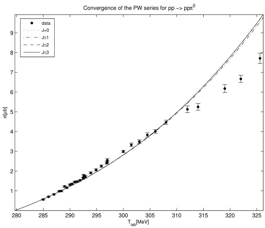
Figure 5.3: Convergence of the partial wave series for $pp\rightarrow pp\pi^{0}$. The dotted, dashed-dotted, dashed and solid line correspond, respectively, to the cross sections with all the contributions up to $J=0$, $J=1$, $J=2$ and $J=3$, as listed in Table 5.4. The nucleon-nucleon interaction is described through the Ohio $NN$ model. The data points are from Ref. [23].

As expected, the importance of the contributions from the channels with higher $J^{\prime}s$ increases with the laboratory energy, $T_{lab}$. Till $\sim 30\mathrm{MeV}$ above threshold, the contributions from the several sets of $J^{\prime}s$ are immaterial compared to the $J=0$ result, which alone describes the data in that energy region. The same conclusions hold when the $NN$ interaction is described through the Bonn B potential[62], due to a smooth variation of the nucleon phase-shifts in that region. We compare in Fig. 5.4 the cross sections with both interactions.

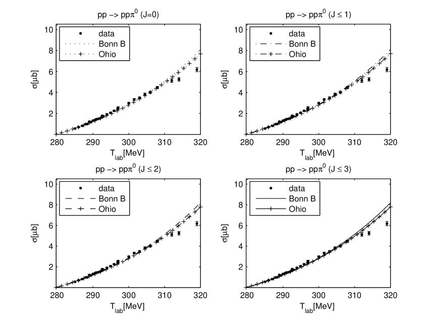
Figure 5.4: Effect of the nucleon-nucleon interaction in the cross section for $pp\rightarrow pp\pi^{0}$. The dotted, dashed-dotted, dashed and solid line correspond, respectively, to the cross section considering the Bonn B potential for the nucleon-nucleon interaction and all the contributions up to $J=0$, $J=1$, $J=2$ and $J=3$. The corresponding lines with +’s consider the nucleon-nucleon interaction to be described by the Ohio $NN$ model. The data points are from Ref. [23].

The cross sections with the Ohio $NN$ model for the nucleon-nucleon interaction (dotted, dashed-dotted, dashed and solid line with +’s) are slightly lower than the ones with the Bonn B potential (dotted, dashed-dotted, dashed and solid lines). Also, naturally, the deviations between the results obtained with the two interactions increase with the energy, and also with $J$.

For $\pi^{-}$ production, the deviation between the cross section with all the contributions up to $J=1$ (dashed-dotted line in Fig. 5.5), $J=2$ (dashed line), and up to $J=3$ (solid line) is very small. However, unlikely to what happens for $\pi^{0}$, the $J=0$ channels (dotted line) are not enough to describe the data in the region of $30\mathrm{MeV}$ above threshold.

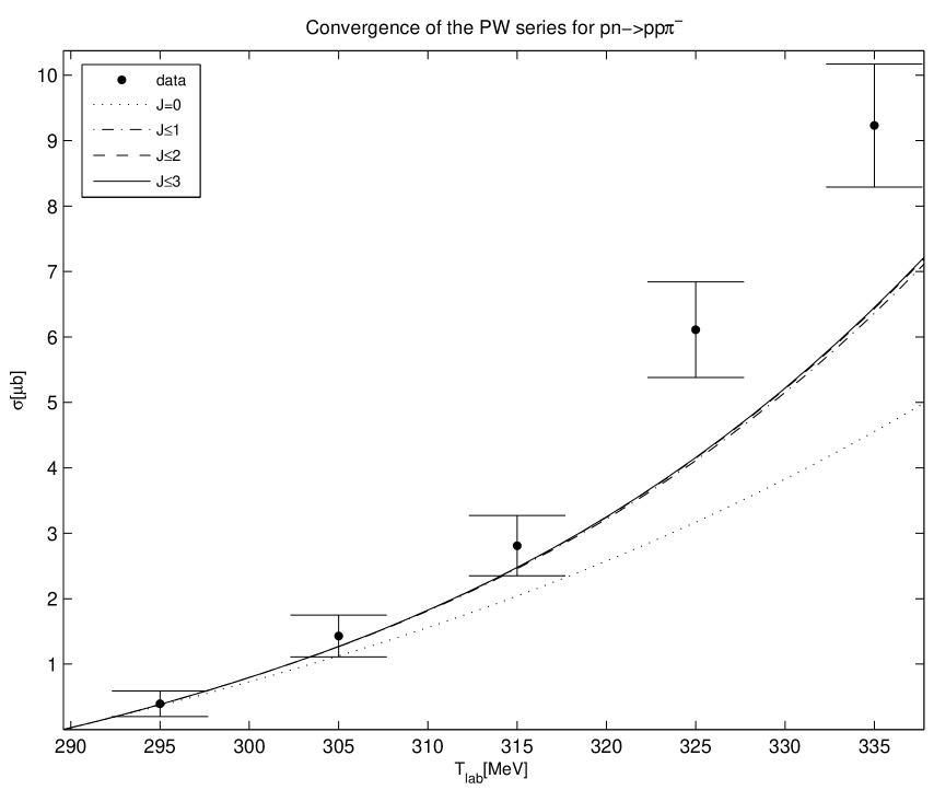
Figure 5.5: Convergence of the partial wave series for $pn\rightarrow pp\pi^{-}$. The meaning of the lines is the same of Fig. 5.3. The data points are from Ref. [32].

The same is found when the $NN$ interaction is described using the Bonn B potential, as it is shown in Fig. 5.6.

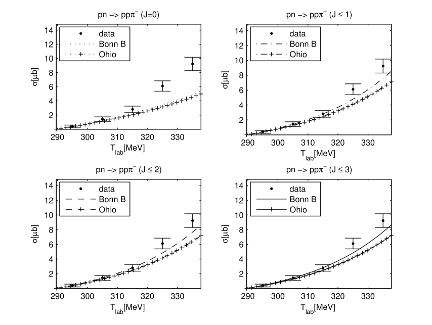
Figure 5.6: Cross section for $pn\rightarrow pp\pi^{-}$ for the Ohio $NN$ model and Bonn B potential for the $NN$ interaction. The meaning of the lines is the same of Fig. 5.4. The data points are from Ref. [32].

We show in Fig. 5.7 the convergence of the partial wave series for the $\pi^{+}$ production. For this reaction, although the convergence is slower, the experimental data near threshold are also described. As already found for $\pi^{-}$ production, since the channels with $J=0$ (dotted line) are not enough to describe the data, one needs to include at least the channels up to $J=2$ (dashed line).

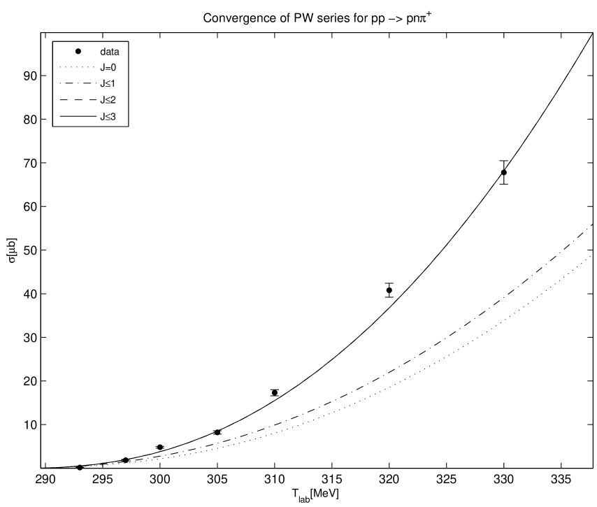
Figure 5.7: Convergence of the partial wave series for $pp\rightarrow pn\pi^{+}$. The meaning of the lines is the same of Fig. 5.3. The data points are from Ref. [28].

Moreover, the $NN$ potential used to describe the $NN$ final- and initial-state interaction can be decisive for the case of $\pi^{+}$ production. We compare in Fig. 5.8 the calculated cross sections with the Bonn B and Ohio interactions, for all sets of $J$’s considered. As expected, the deviation of both results increase with $T_{lab}$ and with $J$, but for this reaction the Bonn B potential fails in describing the data in a much wider region than the Ohio $NN$ model (solid line vs. solid line with +’s in the bottom-right panel of Fig. 5.8).

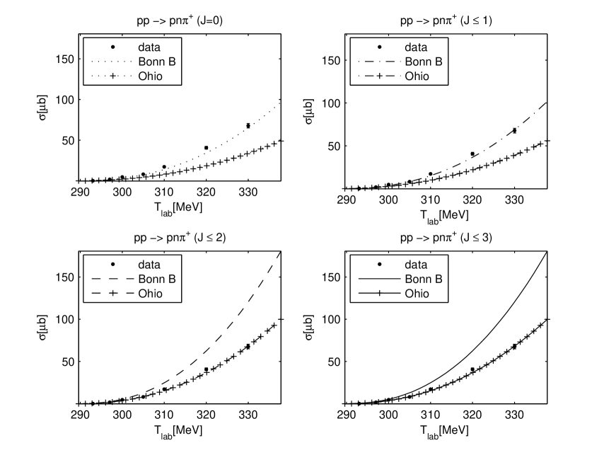
Figure 5.8: Cross section for $pp\rightarrow pn\pi^{+}$ for the Ohio $NN$ model and Bonn B potential for the $NN$ interaction. The data points are from Ref. [28].

5.4 The role of the different production mechanisms

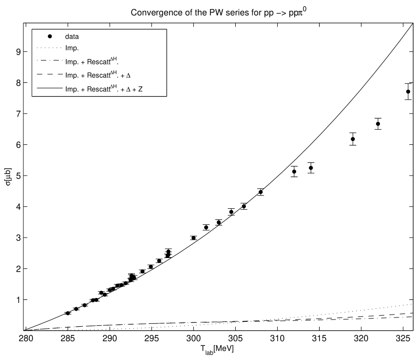
Figure 5.9: Comparison between the contributions for $\pi^{0}$ production of the mechanisms of Fig. 5.1. The dotted line corresponds to the direct-production mechanism alone (diagram a)) and the dashed-dotted line considers the additional contribution of the re-scattering mechanism. In the legend, $\Delta_{H}$ refers to the subtraction of the infinitely heavy limit of Eq. (5.4) from the c_i values of Eq. (5.1.1). The dashed line further includes the explicit $\Delta$-resonance excitation. The solid line represents all the contributions (diagrams a)-d)). The data points are from Ref. [23].

We compare in Fig. 5.9 the contributions of the pion production mechanisms that are illustrated on Fig. 5.1. The direct-production and re-scattering mechanisms alone (dashed-dotted line), highly suppressed, are clearly not enough to describe the $\pi^{0}$ production data. Also, the additional mechanism considering the explicit excitation of a $\Delta$ (dashed line) was found to be small (this is natural, given the discussion in Sec. 5.2.4). As already discussed on Ref. [57], the $Z$-diagrams (solid line) are decisive to remove the discrepancy with the experimental data.

For $\pi^{-}$ production, the re-scattering operator comprises also the Weinberg-Tomozawa term, which does not contribute to $\pi^{0}$ production, and its importance relative to the single nucleon emission term is therefore enhanced (dotted line vs. dashed-dotted line in Fig. 5.10). For this case, the $\Delta$-isobar mechanism is also found to play an important role (dashed line in Fig. 5.10).

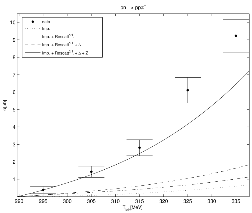
Figure 5.10: Comparison between the contributions for $\pi^{-}$ production of the mechanisms of Fig. 5.1. The meaning of the lines is the same of Fig. 5.9. The re-scattering term now comprises also the Weinberg-Tomozawa mechanism. The data points are from Ref. [32].

The relative importance of the several mechanisms of Fig. 5.1, for $\pi^{+}$ production, is shown in Fig. 5.11, where the re-scattering mechanism is found to contribute significantly (dashed-dotted line).

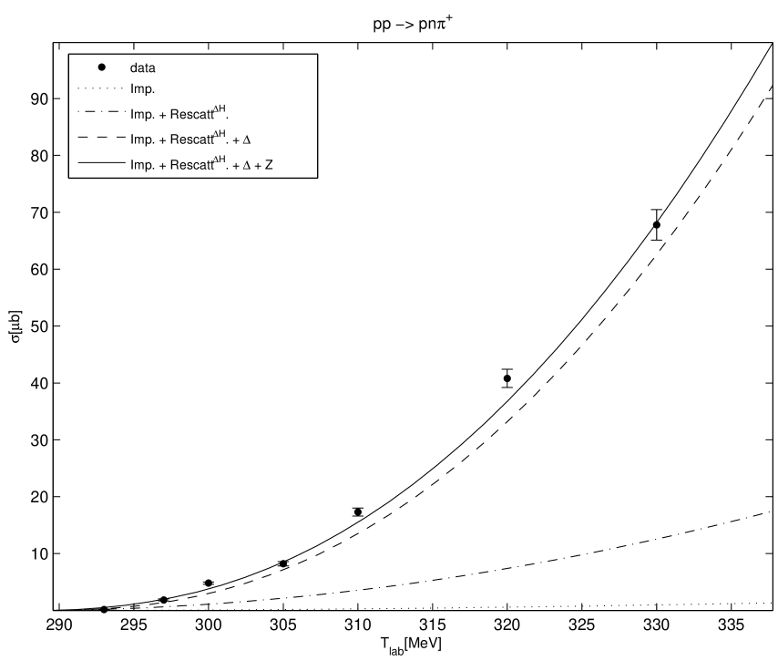
Figure 5.11: The same of Fig. 5.9 but for $pp\rightarrow pn\pi^{+}$. The data points are from Ref. [28].

Since the $\Delta$-resonance is included explicitly in all our calculations, its contribution was subtracted from the values of the low energy constants $c_{i}$’s of the $\pi N$ scattering amplitude in Eq. (5.1.1), which was done taking the infinitely heavy or static limit of Eq. (5.4) (this was indicated by the superscript $\Delta_{H}$ in the legends of Fig. 5.9, Fig. 5.10 and Fig. 5.11). We show in Fig. 5.12 the effect of not including explicitly the mechanism of pion production through the $\Delta$-excitation. In that figure, in contrast to previous ones, the re-scattering amplitude (in the dotted line) is taken with the low energy constant $c_{3}$ including the $\Delta$ contribution. The solid lines are the full calculation for $\pi^{0}$, $\pi^{-}$ and $\pi^{+}$. They coincide with the full lines in Fig. 5.9, Fig. 5.10 and Fig. 5.11, respectively.

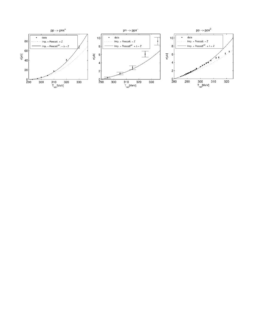
Figure 5.12: Effect on the cross section of not considering the $\Delta$ as an explicit degree of freedom. The solid line is the full calculation of Fig. 5.9-Fig. 5.11 considering the mechanisms of direct-production, re-scattering, $\Delta$-excitation and Z-diagrams (Imp. + Rescatt${}^{\Delta_{H}}$. + $\Delta$ + Z). The dotted line corresponds the calculation with only the direct-production, re-scattering terms and Z diagrams (Imp. + Rescatt. + Z).

For all the cases, the inclusion of the $\Delta$ improves the description of the experimental data. As expected, its importance increases with the energy. Also, both for $\pi^{0}$ and $\pi^{+}$ production, the inclusion of the $\Delta$ increases the cross section. These general trends were already found for the Jülich model[59, 60, 61], presented in Sec. 2.2 (see Fig. 2.8). However, contrarily to this phenomenological model, in which all the short range mechanisms are included through $\omega$-exchange (diagram c) of Fig. 5.1) and adjusted to reproduce the total cross section of the reaction $pp\rightarrow pp\pi^{0}$ close to threshold, in our calculations no adjustment is made, as the parameters for the $Z$-diagrams are taken consistently from the $NN$ interaction employed.

5.5 Importance of the different orbital contributions in the three-body final states

For all the production reactions, the $Ss$ and $Sp$ $\left(NN\right)\pi$ final states were found to be the dominant ones (solid line in Fig. 5.13, Fig. 5.14 and Fig. 5.15 and dotted line in Fig. 5.14 and Fig. 5.15, respectively).

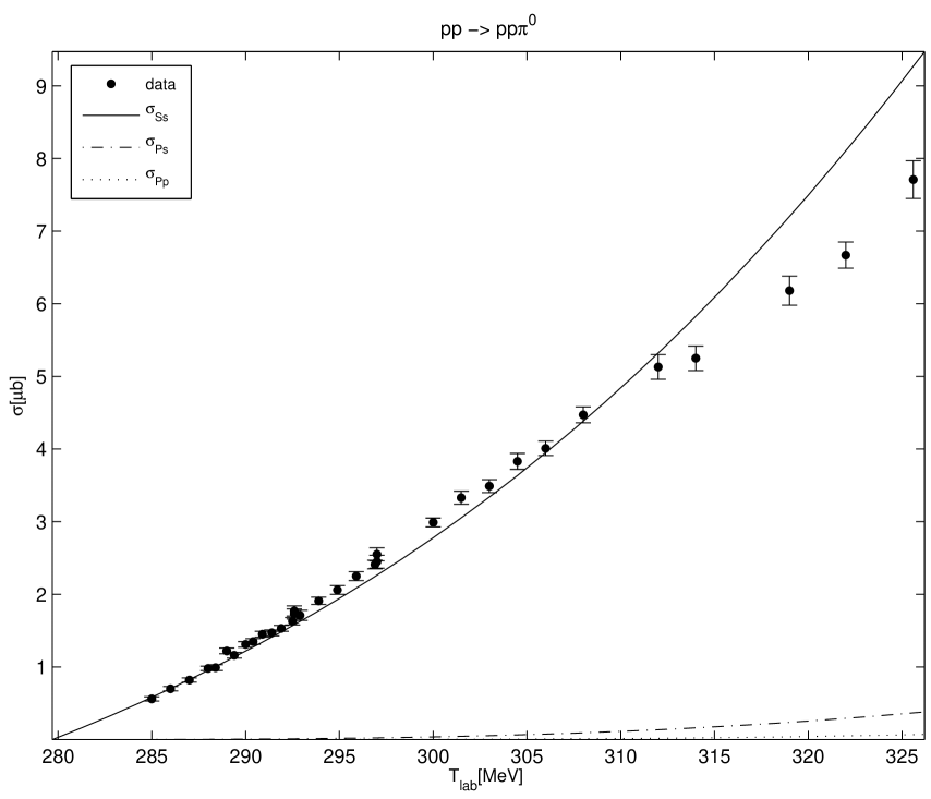
Figure 5.13: Relative importance of the $\left(NN\right)\pi$ final states in $pp\rightarrow pp\pi^{0}$. The cross sections including only the $Ss$, $Ps$ and $Pp$ $\left(NN\right)\pi$ final states are $\sigma_{Ss}$ (solid line), $\sigma_{Ps}$ (dashed-dotted line) and $\sigma_{Pp}$ (dotted line), respectively. The data points are from Ref. [23].

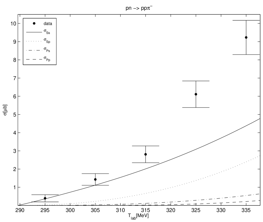
Figure 5.14: Relative importance of the $\left(NN\right)\pi$ final states in $pn\rightarrow pp\pi^{-}$. The cross sections including only the $Ss$, $Sp$ ,$Ps$ and $Pp$ $\left(NN\right)\pi$ final states are $\sigma_{Ss}$ (solid line), $\sigma_{Sp}$ (dotted line), $\sigma_{Ps}$ (dashed-dotted line) and $\sigma_{Pp}$ (dashed line), respectively. The data points are from Ref. [32].

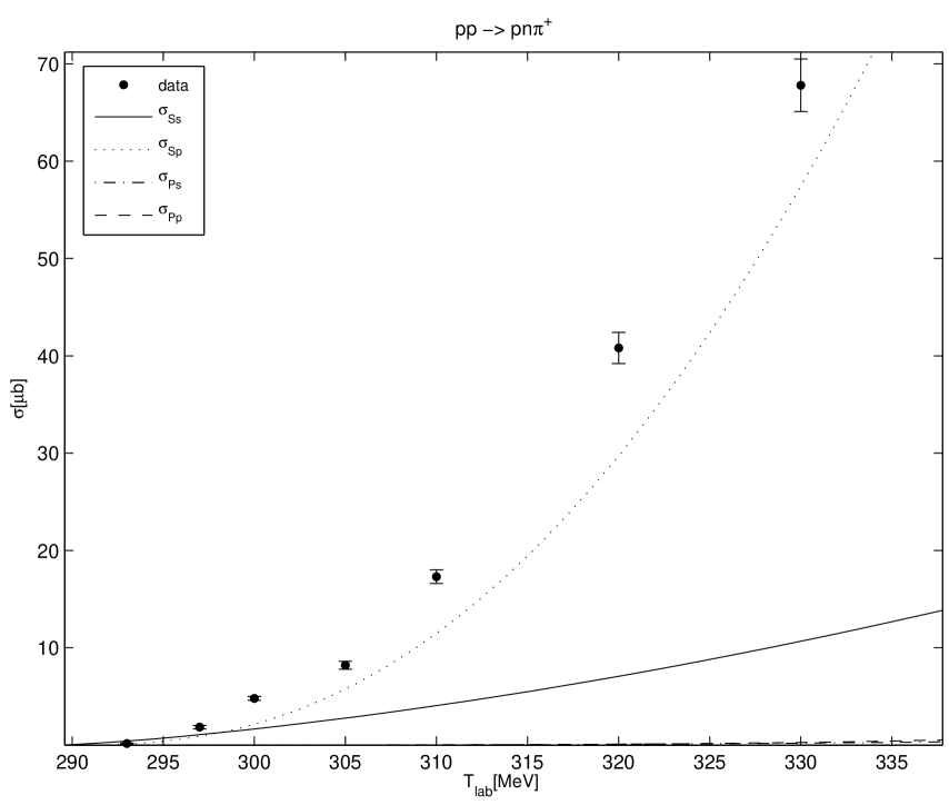
Figure 5.15: Relative importance of the $\left(NN\right)\pi$ final states in $pp\rightarrow pn\pi^{+}$. The meaning of the lines is the same of Fig. 5.14. The data points are from Ref. [28].

In particular, for $\pi^{0}$ production, the cross section with only $Ss$ final states (solid line in Fig. 5.13) is enough to describe the data in a wide energy range. For charged-pion production reactions, the cross section results from an interplay between the $Ss$ final states (which dominate for $\pi^{-}$ production) and the $Sp$ final states (which dominate for $\pi^{+}$ production) (solid and dotted line in Fig. 5.14 and Fig. 5.15).

5.6 Approximations for the energy of the exchanged pion

In this section we start by showing that for all charged pion reaction channels the S-matrix approach for the effective operators, which describe the physical meson production mechanisms, is a very good approximation to the DWBA result obtained directly from TOPT.

We compare in Fig. 5.16 the result from time-ordered perturbation theory to the total cross sections of the several charge production reactions obtained with the on-shell, fixed-kinematics, static and S-matrix approximations. The validity of these approximations has been investigated previously[93] but only for the re-scattering operator and $\pi^{0}$ production (see Chapter 4).

For all the production reactions, the deviation of the S-matrix approach result from the TOPT cross section is much less than the deviations obtained with the other approximations. The maximum deviation, on the other hand, occurs for the static approximation (as checked in Chapter 4, at variance, below threshold, as expected, the static approximation performs better, giving a basis for the traditional static interactions at low energies.)

Figure 5.16: Ratio between the cross section with different energy prescriptions and the TOPT cross section. The dotted, dashed-dotted and dashed line corresponds on-shell approximation, fixed-kinematics and static approximation, respectively. The solid line is the calculation within the S-matrix approach. The Ohio interaction is used for the $NN$ distortions.

We compare in Fig. 5.17, Fig. 5.18 and Fig. 5.19 the effects of the on-shell, fixed-kinematics and static approximations on the total cross section to the result within the S-matrix approach. As expected, these results are in agreement with those shown in Fig. 5.16.

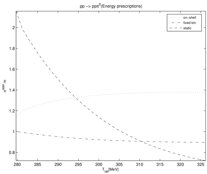
Figure 5.17: Ration between the cross section for $pp\rightarrow pp\pi^{0}$ with different energy prescriptions for the production operator and the S-matrix (coinciding with the “exact” TOPT result, as shown in Fig. 5.16) cross section. The dotted, dashed-dotted and dashed line corresponds on-shell approximation, fixed-kinematics and static approximation, respectively.

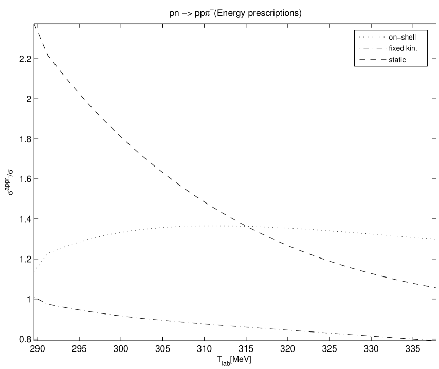
Figure 5.18: The same of Fig. 5.17 but for $pn\rightarrow pp\pi^{-}$.

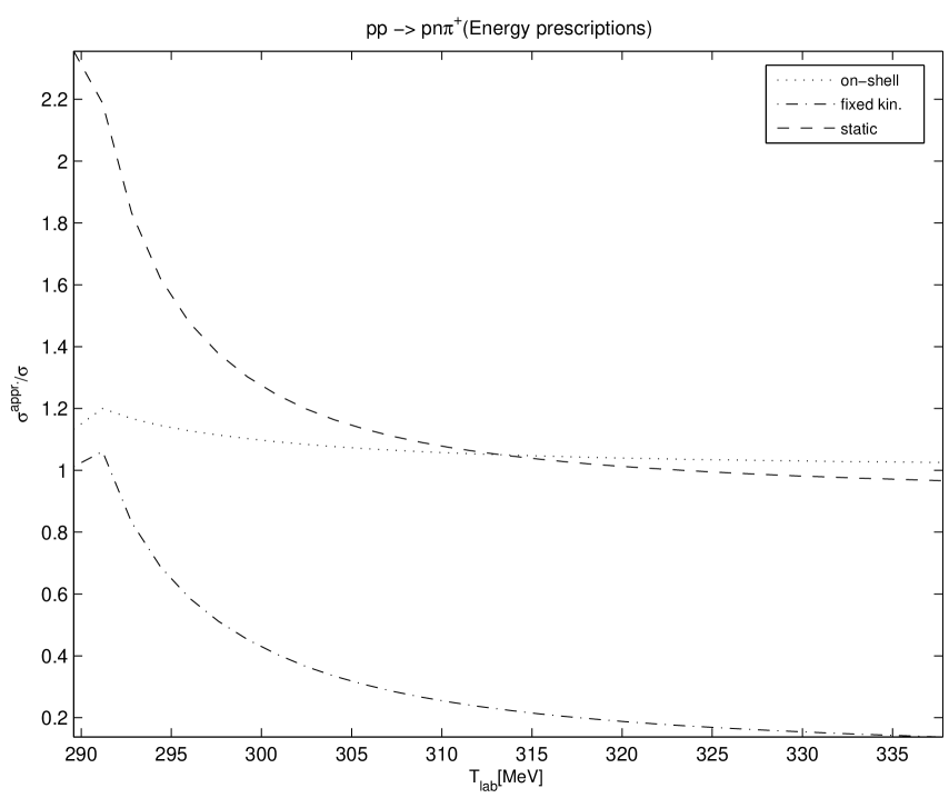
Figure 5.19: The same of Fig. 5.17 but for $pp\rightarrow pn\pi^{+}$.

The deviation from the cross section calculated within the S-matrix approach is maximum for the static approximation, which considers the energy of the exchanged pion to be zero (dashed line). For energies close to threshold, the static approximation overestimates the cross section by a factor larger than $2$. The on-shell approximation (“$E-E^{\prime}$” approximation, which considers the energy of the exchanged pion to be the difference between the nucleon on-shell energies before and after pion emission) deviates also from the reference result, but it may be off $20\%$ for all the charge channels, even for energies close to threshold.

For the $\pi^{0}$ and $\pi^{-}$ production cases (Fig. 5.17 and Fig. 5.18, respectively), about the same happens for the fixed kinematics approximation (energy of the exchanged pion set to its threshold value, $m_{\pi}/2$) as seen in the dashed-dotted lines. As for ${\pi}^{+}$ production, represented in Fig. 5.19, the cross section within the fixed-kinematics approximation is underestimated by a factor of $1.5-2.5$ in the region near threshold, and, for higher energies, by a factor of $\sim 5$.

Our results for $\pi^{+}$ production are consistent with discrepancy with the experimental data reported in Ref. [66], where the calculation also used the $\chi$PT $\pi$N amplitude, but the fixed kinematics approximation was assumed, leading to a calculated cross section which underestimated the data by a factor of $5$ or by a factor of $2$, depending on the $\Delta$ contribution being included or not included[66]. We verified these reduction factors, when the same channels were introduced in our calculation. We furthermore concluded that the deviations observed for the $\pi^{+}$ production reaction are originated by the $p$-waves contributions to the $\pi$N amplitude, as illustrated in Fig. 5.20.

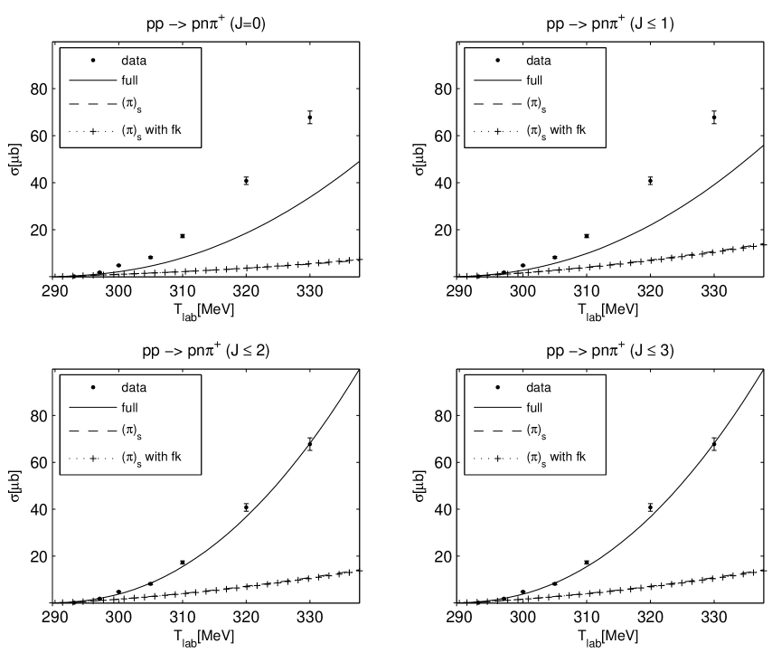
Figure 5.20: Dependence of the effect of the fixed kinematics approximation for the cross section for $pp\rightarrow pn\pi^{+}$ on the orbital $\pi\left(NN\right)$ angular momentum. The solid line is the full calculation. The dashed line is the cross section considering only $s$-wave contributions to the $\pi N$ amplitude. The dotted line with +’s further assumes the fixed kinematics approximation. The Ohio interaction is used for the $NN$ distortions.

In other words, the crucial role of the $\Delta$ in $\pi^{+}$ production enhances the importance of the $\pi N$ $p$-wave states resulting in a slower convergence and in a higher sensitivity to the fixed kinematics approximation.

5.7 Conclusions

This Chapter investigated charged and neutral pion production reactions within the S-matrix approach. The main conclusions are:

1) the S-matrix approach for the description of the pion production operators reproduces numerically the DWBA (TOPT) result. We note that the S-matrix approach simplifies tremendously the numerical effort demanded in TOPT by the presence of logarithmic singularities in the pion propagator for ISI,

2) the contributions from the impulse, re-scattering, $\Delta$-isobar and $Z$-diagrams, within the S-matrix approach successfully describe the cross sections not only for neutral but also for charged pion production, near threshold,

3) the newly developed realistic Ohio $NN$ interaction tuned well above pion production threshold was found to improve the description of the experimental data. For $\pi^{+}$ production, its effect is crucial to reproduce the data in the near-threshold region,

4) the reason for previously reported[66] failures to describe the $pp\rightarrow pn\pi^{+}$ reaction with the $\chi$PT $\pi$N amplitude (giving strengths for the cross section from $1/5$ to $1/2$ of the experimental one) stems from the approximation taken then for the energy of the exchanged pion,

5) convergence of the partial wave series for neutral pion production, and for energies up to $30\mathrm{MeV}$ above threshold, does not require channels with total angular momentum higher than $J=0$. However, for the charged $\pi^{-}$ and $\pi^{+}$ production cases and at the same energies, channels with $J=1$ and $J=2$ at least are needed, due to the importance of $p$ waves in the $\pi N$ and $NN$ interactions, and to the admixtures of both $T=0$ and $T=1$ $NN$ isospin states.

We add that a more detailed description of the experimental data at higher energies may further require a complete coupled-channel $N\Delta$ calculation. The S-matrix approach, shown here to be successful near threshold, should naturally be tested also by the more sensitive polarisation observables and, above all, in high precision calculations, as for instance in charge symmetry breaking studies.

Chapter 6 Conclusions

Understanding pion production, in all its possible charge channels, in nucleon-nucleon collisions near threshold has been a challenge over the last decades. With the experimental data from the new cooler rings, the field entered in a new domain of precision. These unprecedented high quality data on unpolarised, as well as on polarised observables, triggered a plethora of theoretical investigations.

The physics of meson production in nucleon-nucleon collisions is very rich. As the first strong inelasticity for the $NN$ system, the phenomenology of the $NN\rightarrow NN\pi$ reaction is closely linked to that of elastic $NN$ scattering. The fact that low- and medium- energy strong interactions are controlled by chiral symmetry led the hope that chiral effective theories could be used to analyse these processes, and achieve a fundamental understanding of the production processes. This provides the opportunity to improve the phenomenological approaches via matching the chiral expansion and inversely, to constrain the chiral contact terms via resonance saturation. This early excitement was quickly abated by the realisation that proper evaluation within $\chi$PT involves surmounting several severe difficulties, which are caused by the high-momentum transfer nature of this process.

The cross section for the reaction $pp\rightarrow pp\pi^{0}$ near threshold was especially elucidative, since the main pion exchange contribution is there ruled out by isospin conservation. It clearly showed that the transition amplitude results from a delicate interference between the single-nucleon term, the pion re-scattering term, and various additional and individually important contributions from shorter range mechanisms (“Z-diagrams” from heavy meson exchanges). To establish the importance of the latter in an overall description of the different charge channels of pion production, was the main motivation for this work.

DWBA approaches apply a three-dimensional quantum-mechanical formulation for the $NN$ distortion, which is not obtained from the Feynman diagrams describing the production mechanisms. As a consequence, the energy dependence of the pion production operator has been treated approximately and under different prescriptions in calculations performed so far. A clarification of these formal issues was thus needed to enable sound conclusions about the physics of the pion production processes, and it was the aim of Chapters 3 and 4.

Moreover, advance in understanding pion production in $NN$ collisions must follow not from the exclusive study of $pp\rightarrow pp\pi^{0}$, but also from the global understanding of the effects that afflict all channels. Also, to pin down the different production mechanisms, one needs to go beyond the lowest partial waves. These were the main motivations for the work of Chapters 4 and 5.

In short, this thesis aimed to address the problem of charged and neutral pion production in nucleon-nucleon collisions. The main conclusions are:

1. From field theory to DWBA

   The effective pion re-scattering operator was obtained starting from the corresponding four-dimensional Feynman diagram. By integrating over the energy of the exchanged pion, the amplitudes were transformed into those following from time-ordered perturbation theory and could be identified with six time-ordered diagrams.

   From these diagrams, the “stretched box diagrams” (i.e., those with more than one meson in flight in the intermediate states), were seen quantitatively to give a very small contribution, and therefore were neglected. The remaining diagrams were identified with the distorted-wave Born approximation (DWBA) amplitude, allowing to extract an effective production operator. The calculations considered a physical realistic model for pions and nucleons and their interaction vertices.

2. Energy prescriptions for the production operator

   The DWBA amplitude originated by the decomposition of the Feynman diagram into the corresponding time-ordered perturbation theory (TOPT) terms, was used as a reference result to study the commonly used approximations (on-shell, fixed-kinematics and static) for the energy of the exchanged pion. This energy, not fixed in the quantum-mechanical three-dimensional, non-relativistic formalism, was fixed as $\omega_{\pi}$, the on-shell energy of the exchanged pion.

   Near threshold, the retardation effects in the pion re-scattering mechanism were seen to be not very decisive. On the other hand, the effect on the re-scattering vertex alone was found to be significant, largely overestimating the cross section, as unnaturally obtained in previous calculations with ad-hoc choices for the pion energy.

3. The S-matrix approach

   When applying TOPT, each of the re-scattering diagrams for the initial- and final-state distortion defines a different off-energy shell extension of the pion re-scattering amplitude, since energy is not conserved at individual vertices. This imposes the evaluation of two different matrix elements between the quantum-mechanical $NN$ wave functions, for such operators.

   Within the S-matrix technique, however, after the on-shell approximation is made consistently, the pion re-scattering parts of FSI and ISI diagrams coincide and one can identify them with a single effective re-scattering operator.

   The amplitudes and cross sections obtained with the S-matrix effective operator were verified to be very close to those calculated with the “exact” TOPT result, up to $150\mathrm{MeV}$ above threshold.

4. Charged and neutral pion production

   If one considers the contributions from the single-nucleon emission term, re-scattering, $\Delta$-isobar and $Z$-diagrams, the S-matrix approach successfully describes the cross sections for both neutral and charged pion production, near threshold.
   The S-matrix approach reproduces numerically the results from TOPT.

   For neutral (charged) pion production, the summation of all channels up to total angular momentum $J=0$ ($J=2$) is enough up to $30\mathrm{MeV}$.

   The $NN$ interaction was found to be decisive to reproduce the data in the near-threshold region (in particular for $\pi^{+}$ production). In this channel we found also that the correct treatment of the exchanged pion energy in the re-scattering term beyond the fixed kinematics approximation, is essential to remove the previously reported too low cross section strength.

   In the overall, even for energies close to threshold, the cross sections with the approximations for the energy of the exchanged pion other than the S-matrix, deviate at least $20\%$ from the full calculation, being larger for the $\pi^{+}$ channel.

Our findings for the cross section are in agreement with those of the Jülich model. However, contrarily to this approach, for which all the short range mechanisms are included only through $\omega$-exchange and adjusted to reproduce the total cross section of the reaction $pp\rightarrow pp\pi^{0}$ close to threshold, in our calculations no adjustment is made, as the parameters for the $Z$-diagrams are taken consistently from the $NN$ interaction employed, providing a good description of all charge channels.

There are several issues which would undoubtedly be a step further in the investigations of this thesis. Since the importance of the $\Delta$ contribution increases with energy, a detailed description of the experimental data in regions of higher energy may further require a complete coupled-channel $N\Delta$ calculation. Also, although the effect of other higher mass nucleon resonances was found to be small, these mechanisms should also be considered in future calculations.

Moreover, the S-matrix approach, which successfully describes the near-threshold cross sections for neutral and charged pion production, should be submitted to the most stringent test of describing pion (and other mesons) polarisation observables. Finally, since the S-matrix approach passed so well the test of pion production, it is natural to extend the method to the $\eta$ meson sector.

In recent years, the improvement of experimental facilities, detectors and accelerators permitted the acquisition of a great deal of high-precision data, leading to the improvement of its theoretical understanding (both in $\chi$PT and in other phenomenological approaches), and are a promise of very exciting times to come in the near future of meson production physics, where for instance, $\eta$ and $\eta^{\prime}$ production still pose interesting problems.

Appendix A General remarks on kinematics

Fig. A.1 illustrates the choice of variables adopted in this work.

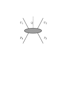
Figure A.1: Illustration of the choice of variables for $NN\rightarrow NN\pi$. The solid lines and dashed lines represent the nucleon and pion, respectively. The initial(final) nucleon four-momenta are $P_{1}$ and $P_{2}$$\left(U_{1}\text{ and }U_{2}\right)$. The four-momentum of the produced pion is $Q$.

Final and initial momenta

The initial nucleon four-momenta in the overall centre of mass system are given by

$$P_{1} = \left(E_{1},\vec{p}\right)$$ (A.1)

$$P_{2} = \left(E_{2},-\vec{p}\right),$$ (A.2)

with $E_{1,2}=\sqrt{M^{2}+p^{2}}\equiv E$. For energies close to the pion production threshold, the non-relativistic expressions for the energy of the final nucleons can be used. Thus, in the centre-of-mass of the final three-body system,

$$U_{1} = \left(F_{1},\vec{q}_{u}-\frac{\vec{q}_{\pi}}{2}\right)$$ (A.3)

$$U_{2} = \left(F_{2},-\vec{q}_{u}-\frac{\vec{q}_{\pi}}{2}\right),$$ (A.4)

where $\vec{q}_{u}$ is the relative momentum of the final nucleons and $\vec{q}_{\pi}$ is the centre-of-mass momentum of the produced pion. From energy conservation it follows that

$$2E = F_{1}+F_{2}+E_{\pi}$$ (A.5)

$$\approx 2M+\frac{q_{u}^{2}}{2\mu}+\frac{q_{\pi}^{2}}{4M}+\sqrt{m_{\pi}^{2}+q_{\pi}^{2}}.$$ (A.6)

Laboratory energy and maximum pion momentum

For the kinematics of the pion production reactions investigated in this work, the nucleons were considered as having equal masses ($M$). The laboratory energy can then be determined from

$$T_{lab}=\frac{s-4M^{2}}{2M},$$ (A.7)

with $s\equiv\left(P_{1}+P_{2}\right)^{2}$. The excess energy $Q$ is given by

$$Q=\sqrt{s}-\left(2M+m_{\pi}\right).$$ (A.8)

The maximum pion momentum, which occurs when $q_{u}=0$, can be calculated (in units of $m_{\pi}$) using

$$\eta=\frac{1}{m_{\pi}}\left[\frac{1}{2\sqrt{s}}\sqrt{\left(s-m_{\pi}^{2}-4M^{2}\right)^{2}-16M^{2}m_{\pi}^{2}}\right].$$ (A.9)

Eqs. (A.7), (A.8) and (A.9) can be easily generalised for the case when the nucleons have different masses[1]:

$$T_{lab}=\frac{s-M_{i1}^{2}-M_{i2}^{2}-2M_{i1}M_{i2}}{2M_{i1}},$$ (A.10)

$$Q=\sqrt{s}-\left(M_{f1}+M_{f2}+m_{\pi}\right),$$ (A.11)

and

$$\eta=\frac{1}{m_{\pi}}\left[\frac{1}{2\sqrt{s}}\sqrt{\left(s-m_{\pi}^{2}-M^{2}_{f}\right)^{2}-4M^{2}_{f}m_{\pi}^{2}}\right].$$ (A.12)

where the masses of the initial (final) nucleons are $M_{i1}$ and $M_{i2}$ ($M_{f1}$ and $M_{f2}$), and $M_{f}=M_{f1}+M_{f2}$.

It is important to remark that the relativistic and non relativistic calculations of the threshold laboratory energy $T_{thr.}$ differ significantly,

$$T_{thr.}^{Rel.} = \frac{4M^{2}+4Mm_{\pi}+m_{\pi}^{2}-4M^{2}}{2M}$$ (A.13)

$$= 2m_{\pi}+\left(\frac{m_{\pi}^{2}}{2M}\right)$$ (A.14)

$$= T_{thr.}^{NRel.}+\left(\frac{m_{\pi}^{2}}{2M}\right),$$ (A.15)

since $\left(\frac{m_{\pi}^{2}}{2M}\right)\approx 10\mathrm{MeV}$. This difference can have decisive effects on the results, especially at threshold.

Appendix B Kinematic definitions for the diagrams

Re-scattering diagram

The kinematic conventions adopted for the re-scattering diagram are represented on Fig. B.1. The relations resulting from four-momentum conservation are listed on Table B.1.

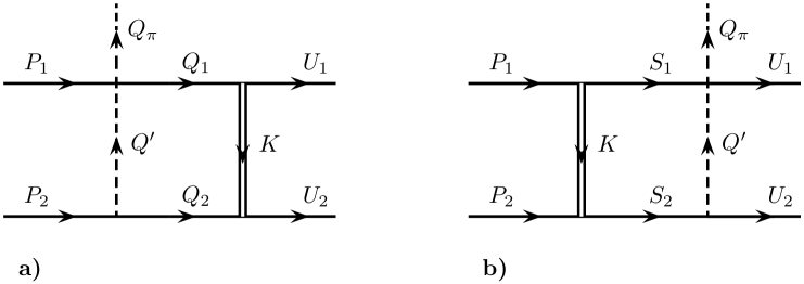
Figure B.1: Illustration of the choice of variables for the re-scattering diagram for a) FSI and b) ISI. The solid lines and dashed lines represent the nucleon and pion, respectively. The initial(final) nucleon four-momenta are $P_{1}$ and $P_{2}$$\left(U_{1}\text{ and }U_{2}\right)$. The four-momentum of the produced pion is $Q_{\pi}$. The four-momentum of the exchanged pion($\sigma$ meson) is $Q^{\prime}$$\left(K\right)$. The four-momenta of the intermediate nucleons for the FSI(ISI) case are $Q_{1}\text{ and }Q_{2}$$\left(S_{1}\text{ and }S_{2}\right)$.

FSI	ISI
$P_{1}+Q^{\prime}-Q_{\pi}-Q_{1}=0\hskip 24.18501pt$	$P_{1}-K-S_{1}=0$
$P_{2}-Q^{\prime}-Q_{2}=0$	$P_{2}+K-S_{2}=0$
$Q_{1}-K-U_{1}=0$	$S_{1}+Q^{\prime}-Q_{\pi}-U_{1}=0$
$Q_{2}+K-U_{2}=0$	$S_{2}-Q^{\prime}-U_{2}=0$

Table B.1: Four-momentum conservation for the re-scattering diagram.

For the final state $NN$ interaction (diagram a) of Fig. B.1), the expressions for the on-shell energies of the particles are:

$$\omega_{\pi}=\sqrt{m_{\pi}^{2}+\left|-\vec{p}+\frac{\overrightarrow{q_{\pi}}}{2}+\overrightarrow{q_{k}}\right|^{2}}\text{\hskip 33.28966ptexchanged }\pi$$ (B.1)

$$\omega_{2,1}=\sqrt{M^{2}+\left|\overrightarrow{q_{k}}\text{$\pm$}\frac{\overrightarrow{q_{\pi}}}{2}\right|^{2}}\hskip 56.9055pt\text{intermediate nucleons}$$ (B.2)

$$\omega_{\sigma}=\sqrt{m_{\sigma}^{2}+\left|\overrightarrow{q_{k}}-\overrightarrow{q_{u}}\right|^{2}}\text{\hskip 68.00206pt}\sigma\text{ exchanged}$$ (B.3)

$$F_{2,1}=M+\frac{1}{2M}\left|\overrightarrow{q_{u}}\text{$\pm$}\frac{\overrightarrow{q_{\pi}}}{2}\right|^{2}\hskip 48.65439pt\text{final nucleons}$$ (B.4)

and, for the initial $NN$ interaction, the corresponding expressions are

$$\omega_{\pi}=\sqrt{m_{\pi}^{2}+\left|\overrightarrow{q_{u}}+\frac{\overrightarrow{q_{\pi}}}{2}-\overrightarrow{q_{k}}\right|^{2}}\text{\hskip 33.57404ptexchanged }\pi$$ (B.5)

$$\omega_{1,2}=\sqrt{M^{2}+\left|\overrightarrow{q_{k}}\right|^{2}}\hskip 84.22034pt\text{intermediate nucleons}$$ (B.6)

$$\omega_{\sigma}=\sqrt{m_{\sigma}^{2}+\left|\overrightarrow{p}-\overrightarrow{q_{k}}\right|^{2}}\text{\hskip 67.7177pt}\sigma\text{ exchanged}$$ (B.7)

$$F_{2,1}=M+\frac{1}{2M}\left|\overrightarrow{q_{u}}\text{$\pm$}\frac{\overrightarrow{q_{\pi}}}{2}\right|^{2}\hskip 48.36958pt\text{final nucleons}$$ (B.8)

where $\vec{p}$ and $\overrightarrow{q_{\pi}}$ are the initial nucleon three-momentum and the emitted pion three-momentum, respectively. The relative three-momentum of the two intermediate(final) nucleons is $\overrightarrow{q_{k}}\left(\overrightarrow{q_{u}}\right)$, and the energy of the emitted pion is $E_{\pi}=\sqrt{m_{\pi}^{2}+\left|\overrightarrow{q_{\pi}}\right|^{2}}$. The nucleon, the pion and the $\sigma$ mass are $M$, $m_{\pi}$ and $m_{\sigma}$, respectively. All quantities are referred to the three-body centre-of-mass frame of the $\pi NN$ final state.

Direct-production diagram

The kinematic conventions adopted for the direct-production diagram are represented on Fig. B.2. The relations resulting from four-momentum conservation are listed on Table B.2.

Figure B.2: Illustration of the choice of variables for the direct-production diagram for a) FSI and b) ISI. The meaning of the variables is the same of Fig. B.1.

FSI	ISI
$P_{1}-Q_{\pi}-Q_{1}=0\hskip 24.18501pt$	$P_{1}-K-S_{1}=0$
$Q_{1}-K-U_{1}=0$	$S_{1}-Q_{\pi}-U_{1}=0$
$P_{2}+K-U_{2}=0$	$P_{2}+K-U_{2}=0$

Table B.2: Four-momentum conservation for the direct-production diagram.

The expressions for the on-shell energies can be easily obtained from Eq. (B.1)-Eq. (B.4) and Eq. (B.5)-Eq. (B.8).

Appendix C Partial fraction decomposition and TOPT

For the loop diagrams considered in this work, we have in general to evaluate integrals like

$$\mathcal{M}=\int\frac{dQ_{0}^{\prime}}{\left(2\pi\right)}f\left(Q_{0}^{\prime}\right)\times U_{1}L_{1}\times U_{2}L_{2}\times U_{3}L_{3}$$ (C.1)

where $U_{i}$, $L_{i}$ are terms with the poles in the upper-half plan and in the lower half-plan, respectively, which can be generically written as:

$$U_{i}=\frac{1}{Q_{0}^{\prime}-u_{i}-i\varepsilon}\hskip 85.35826ptL_{i}=\frac{1}{Q_{0}^{\prime}-l_{i}+i\varepsilon},$$ (C.2)

and $f\left(Q_{0}^{\prime}\right)$ is a generic vertex function which depends on the momentum of one of the exchanged particles.

Direct integration of Eq. (C.1) by closing the contour in one of the half-plans and picking up the poles enclosed, give as a result an expression where one has to evaluate the vertex $f$ for three different energies (the pole contributions) of the exchanged particle $Q_{0}^{\prime}$. For instance, if we close the contour in the upper half-plan, $f$ must be calculated for $Q_{0}^{\prime}=u_{1}$, $Q_{0}^{\prime}=u_{2}$ and $Q_{0}^{\prime}=u_{3}$. We thus gain little insight on the adequate choice to be done for $Q_{0}^{\prime}$ in the traditional three-dimensional formalisms, where this energy is not fixed.

However, by performing a partial fraction decomposition of the integrand before integrating in $Q_{0}^{\prime}$, provides us a visible connection with time-ordered perturbation theory. The way the partial fraction decomposition is done ensures that we have only contributions from terms with one pole on the on-shell energy of the particle interacting through $f\left(Q_{0}^{\prime}\right)$ and the remaining one or two poles in the other half-plan. Closing the contour in the half-plan where there is only one pole, we can relate directly $Q_{0}^{\prime}$ at the vertex with the on-shell energy of the considered particle. Of course, the final result must not depend on the method adopted for integration.

Let $u_{3}$ and $l_{3}$ be the poles we want to isolate. We start by writing the product $U_{3}L_{3}$ as a difference of two terms

$$U_{3}L_{3}=\alpha_{33}\left(U_{3}-L_{3}\right)\hskip 28.45274pt\text{with}\hskip 28.45274pt\alpha_{33}\equiv\frac{1}{u_{3}-l_{3}}\text{,}$$ (C.3)

and doing the same for the terms concerning the other exchanged particle, $U_{2}L_{2}$:

$$U_{2}L_{2}=\alpha_{22}\left(U_{2}-L_{2}\right)\hskip 28.45274pt\text{with}\hskip 28.45274pt\alpha_{22}\equiv\frac{1}{u_{2}-l_{2}}$$ (C.4)

Then Eq. (C.1) reads

$$\mathcal{M} = \int\frac{dQ_{0}^{\prime}}{\left(2\pi\right)}f\left(Q_{0}^{\prime}\right)\alpha_{22}\alpha_{33}U_{1}L_{1}U_{2}U_{3}-\int\frac{dQ_{0}^{\prime}}{\left(2\pi\right)}f\left(Q_{0}^{\prime}\right)\alpha_{22}\alpha_{33}U_{1}L_{1}U_{2}L_{3}$$ (C.6)

$$-\int\frac{dQ_{0}^{\prime}}{\left(2\pi\right)}f\left(Q_{0}^{\prime}\right)\alpha_{22}\alpha_{33}U_{1}L_{1}L_{2}U_{3}+\int\frac{dQ_{0}^{\prime}}{\left(2\pi\right)}f\left(Q_{0}^{\prime}\right)\alpha_{22}\alpha_{33}U_{1}L_{1}L_{2}L_{3}$$

Now, in  (C.6), we apart $L_{1}U_{2}$ and in  (C.6), we apart $U_{1}L_{2}$,

$$\mathcal{M} = \int\frac{dQ_{0}^{\prime}}{\left(2\pi\right)}f\left(Q_{0}^{\prime}\right)\alpha_{22}\alpha_{33}\alpha_{21}U_{1}U_{2}U_{3}$$ (C.14)

$$-\int\frac{dQ_{0}^{\prime}}{\left(2\pi\right)}f\left(Q_{0}^{\prime}\right)\alpha_{22}\alpha_{33}\alpha_{21}U_{1}L_{1}U_{3}$$

$$-\int\frac{dQ_{0}^{\prime}}{\left(2\pi\right)}f\left(Q_{0}^{\prime}\right)\alpha_{22}\alpha_{33}\alpha_{21}U_{1}U_{2}L_{3}$$

$$+\int\frac{dQ_{0}^{\prime}}{\left(2\pi\right)}f\left(Q_{0}^{\prime}\right)\alpha_{22}\alpha_{33}\alpha_{21}U_{1}L_{1}L_{3}$$

$$-\int\frac{dQ_{0}^{\prime}}{\left(2\pi\right)}f\left(Q_{0}^{\prime}\right)\alpha_{22}\alpha_{33}\alpha_{12}U_{1}L_{1}U_{3}$$

$$+\int\frac{dQ_{0}^{\prime}}{\left(2\pi\right)}f\left(Q_{0}^{\prime}\right)\alpha_{22}\alpha_{33}\alpha_{12}L_{2}L_{1}U_{3}$$

$$+\int\frac{dQ_{0}^{\prime}}{\left(2\pi\right)}f\left(Q_{0}^{\prime}\right)\alpha_{22}\alpha_{33}\alpha_{12}U_{1}L_{1}L_{3}$$

$$-\int\frac{dQ_{0}^{\prime}}{\left(2\pi\right)}f\left(Q_{0}^{\prime}\right)\alpha_{22}\alpha_{33}\alpha_{12}L_{2}L_{1}L_{3}$$

and finally, in  (C.14),  (C.14),  (C.14) and  (C.14), we apart $U_{1}L_{1}$:

$$\mathcal{M} =\int\frac{dQ_{0}^{\prime}}{\left(2\pi\right)}f\left(Q_{0}^{\prime}\right)\alpha_{22}\alpha_{33}\alpha_{21}U_{1}U_{2}U_{3}$$ (C.18)

$$-\int\frac{dQ_{0}^{\prime}}{\left(2\pi\right)}f\left(Q_{0}^{\prime}\right)\alpha_{22}\alpha_{33}\alpha_{21}\alpha_{11}U_{1}U_{3}+\int\frac{dQ_{0}^{\prime}}{\left(2\pi\right)}f\left(Q_{0}^{\prime}\right)\alpha_{22}\alpha_{33}\alpha_{21}\alpha_{11}L_{1}U_{3}$$

$$-\int\frac{dQ_{0}^{\prime}}{\left(2\pi\right)}f\left(Q_{0}^{\prime}\right)\alpha_{22}\alpha_{33}\alpha_{21}U_{1}U_{2}L_{3}$$

$$+\int\frac{dQ_{0}^{\prime}}{\left(2\pi\right)}f\left(Q_{0}^{\prime}\right)\alpha_{22}\alpha_{33}\alpha_{21}\alpha_{11}U_{1}L_{3}-\int\frac{dQ_{0}^{\prime}}{\left(2\pi\right)}f\left(Q_{0}^{\prime}\right)\alpha_{22}\alpha_{33}\alpha_{21}\alpha_{11}L_{1}L_{3}$$

$$-\int\frac{dQ_{0}^{\prime}}{\left(2\pi\right)}f\left(Q_{0}^{\prime}\right)\alpha_{22}\alpha_{33}\alpha_{12}\alpha_{11}U_{1}U_{3}+\int\frac{dQ_{0}^{\prime}}{\left(2\pi\right)}f\left(Q_{0}^{\prime}\right)\alpha_{22}\alpha_{33}\alpha_{12}\alpha_{11}L_{1}U_{3}$$ (C.19)

$$+\int\frac{dQ_{0}^{\prime}}{\left(2\pi\right)}f\left(Q_{0}^{\prime}\right)\alpha_{22}\alpha_{33}\alpha_{12}L_{1}L_{2}U_{3}$$ (C.20)

$$+\int\frac{dQ_{0}^{\prime}}{\left(2\pi\right)}f\left(Q_{0}^{\prime}\right)\alpha_{22}\alpha_{33}\alpha_{12}\alpha_{11}U_{1}L_{3}-\int\frac{dQ_{0}^{\prime}}{\left(2\pi\right)}f\left(Q_{0}^{\prime}\right)\alpha_{22}\alpha_{33}\alpha_{12}\alpha_{11}L_{1}L_{3}$$ (C.21)

$$-\int\frac{dQ_{0}^{\prime}}{\left(2\pi\right)}f\left(Q_{0}^{\prime}\right)\alpha_{22}\alpha_{33}\alpha_{12}L_{2}L_{1}L_{3}$$ (C.22)

where, accordingly to our conventions, $\alpha_{ij}\equiv\frac{1}{u_{i}-l_{j}}$.

$\mathcal{M}$ is written as a sum of eight types of terms: terms with three-poles in the upper-half plan  (C.18) or in the lower half-plan  (C.22); with two poles in the upper half-plan (first term of  (C.18) and  (C.19)) or in the lower half-plan (second term of  (C.18) and  (C.21)); with one pole in each half-plan (second term of  (C.18) and  (C.19) and first term of  (C.18) and  (C.21)); and finally, terms with two poles in the upper half-plan and one in the lower half-plan  (C.18) or vice-versa  (C.20). The corresponding schematic is represented on Fig. 3.2.

Assuming that the integrals with all the poles in the same half-plan vanish (which happens if $f\left(Q_{0}^{\prime}\right)$ is linear in $Q_{0}^{\prime}$), $\mathcal{M}$ is reduced to only six terms:

$$\mathcal{M} = \int\frac{dQ_{0}^{\prime}}{\left(2\pi\right)}f\left(Q_{0}^{\prime}\right)\alpha_{22}\alpha_{33}\alpha_{21}\alpha_{11}L_{1}U_{3}+\int\frac{dQ_{0}^{\prime}}{\left(2\pi\right)}f\left(Q_{0}^{\prime}\right)\alpha_{22}\alpha_{33}\alpha_{12}\alpha_{11}L_{1}U_{3}$$ (C.25)

$$+\int\frac{dQ_{0}^{\prime}}{\left(2\pi\right)}f\left(Q_{0}^{\prime}\right)\alpha_{22}\alpha_{33}\alpha_{21}\alpha_{11}U_{1}L_{3}+\int\frac{dQ_{0}^{\prime}}{\left(2\pi\right)}f\left(Q_{0}^{\prime}\right)\alpha_{22}\alpha_{33}\alpha_{12}\alpha_{11}U_{1}L_{3}$$

$$+\int\frac{dQ_{0}^{\prime}}{\left(2\pi\right)}f\left(Q_{0}^{\prime}\right)\alpha_{22}\alpha_{33}\alpha_{12}L_{1}L_{2}U_{3}-\int\frac{dQ_{0}^{\prime}}{\left(2\pi\right)}f\left(Q_{0}^{\prime}\right)\alpha_{22}\alpha_{33}\alpha_{21}U_{1}U_{2}L_{3}$$

These terms can be directly identified with the ones resulting from TOPT. More precisely,  (C.25)- (C.25) can be identified with the DWBA terms and  (C.25) with the stretched boxes, as is illustrated on Fig. 3.4 for the FSI case.

The next section exemplifies this method for the FSI case.

Re-scattering diagram with final state interaction

From Eq. (3.1.1) we have

$$\left\{\begin{array}[c]{l}u_{1}=E_{2}-\omega_{2}+i\varepsilon\\ u_{2}=E_{2}-F_{2}-\omega_{\sigma}+i\varepsilon\\ u_{3}=-\omega_{\pi}+i\varepsilon\end{array}\right.\qquad\text{and}\qquad\left\{\begin{array}[c]{l}l_{1}=E_{\pi}+\omega_{1}-E_{1}-i\varepsilon\\ l_{2}=E_{2}-F_{2}+\omega_{\sigma}-i\varepsilon\\ l_{3}=\omega_{\pi}-i\varepsilon\end{array}\right.$$ (C.26)

and consequently,

$$\frac{1}{\alpha_{11}} \equiv u_{1}-l_{1}=E_{tot}-E_{\pi}-\omega_{1}-\omega_{2}+2i\varepsilon$$ (C.27)

$$\frac{1}{\alpha_{22}} \equiv u_{2}-l_{2}=-2\omega_{\sigma}+2i\varepsilon$$ (C.28)

$$\frac{1}{\alpha_{33}} \equiv u_{3}-l_{3}=-2\omega_{\pi}+2i\varepsilon$$ (C.29)

$$\frac{1}{\alpha_{12}} \equiv u_{1}-l_{2}=F_{2}-\omega_{2}-\omega_{\sigma}=E_{tot}-F_{1}-E_{\pi}-\omega_{2}-\omega_{\sigma}+2i\varepsilon$$ (C.30)

$$\frac{1}{\alpha_{21}} \equiv u_{2}-l_{1}=E_{tot}-F_{2}-E_{\pi}-\omega_{1}-\omega_{\sigma}+2i\varepsilon$$ (C.31)

with $E_{tot}=E_{1}+E_{2}=F_{1}+F_{2}+E_{\pi}$ . The residues of $U_{1}$, $U_{2}$, $L_{1}$ and $L_{2}$ are

$$\text{Res}\left.\vskip 12.0pt plus 4.0pt minus 4.0ptU_{1}\right|_{Q_{0}^{\prime}=l_{3}}=\frac{1}{l_{3}-u_{1}}=-\frac{1}{E_{2}-\omega_{2}-\omega_{\pi}}=-\frac{1}{E_{tot}-E_{1}-\omega_{2}-\omega_{\pi}}\hskip 85.35826pt$$ (C.32)

$$\text{Res}\left.\vskip 12.0pt plus 4.0pt minus 4.0ptU_{2}\right|_{Q_{0}^{\prime}=l_{3}}=\frac{1}{l_{3}-u_{2}}=-\frac{1}{E_{2}-F_{2}-\omega_{\sigma}-\omega_{\pi}}=-\frac{1}{E_{tot}-E_{1}-F_{2}-\omega_{\sigma}-\omega_{\pi}}$$ (C.33)

and

$$\text{Res}\left.\vskip 12.0pt plus 4.0pt minus 4.0ptL_{1}\right|_{Q_{0}^{\prime}=u_{3}}=\frac{1}{u_{3}-l_{1}}=\frac{1}{E_{1}-E_{\pi}-\omega_{1}-\omega_{\pi}}=\frac{1}{E_{tot}-E_{2}-E_{\pi}-\omega_{1}-\omega_{\pi}}\hskip 85.35826pt$$ (C.34)

$$\text{Res}\left.\vskip 12.0pt plus 4.0pt minus 4.0ptL_{2}\right|_{Q_{0}^{\prime}=u_{3}}=\frac{1}{u_{3}-l_{2}}=\frac{1}{F_{2}-E_{2}-\omega_{\sigma}-\omega_{\pi}}=\frac{1}{E_{tot}-F_{1}-E_{\pi}-E_{2}-\omega_{\sigma}-\omega_{\pi}}$$ (C.35)

Therefore, the amplitude Eq. (3.1.1) reads:

$$\mathcal{M}^{FSI}_{TOPT}=-g_{\sigma}^{2}\int\frac{d^{3}q^{\prime}}{\left(2\pi\right)^{3}}\frac{1}{4\omega_{\sigma}\omega_{\pi}}\times$$ (C.36)

$$\left[\frac{f\left(\omega_{\pi}\right)}{\left(E_{tot}-E_{\pi}-\omega_{1}-\omega_{2}\right)\left(E_{tot}-E_{1}-\omega_{2}-\omega_{\pi}\right)\left(E_{tot}-F_{1}-E_{\pi}-\omega_{2}-\omega_{\sigma}\right)}\right.$$

$$\left.+\frac{f\left(\omega_{\pi}\right)}{\left(E_{tot}-E_{\pi}-\omega_{1}-\omega_{2}\right)\left(E_{tot}-E_{1}-\omega_{2}-\omega_{\pi}\right)\left(E_{tot}-F_{2}-E_{\pi}-\omega_{1}-\omega_{\sigma}\right)}\right.$$

$$\left.+\frac{f\left(-\omega_{\pi}\right)}{\left(E_{tot}-E_{\pi}-\omega_{1}-\omega_{2}\right)\left(E_{tot}-E_{2}-E_{\pi}-\omega_{1}-\omega_{\pi}\right)\left(E_{tot}-F_{1}-E_{\pi}-\omega_{2}-\omega_{\sigma}\right)}\right.$$

$$\left.+\frac{f\left(-\omega_{\pi}\right)}{\left(E_{tot}-E_{\pi}-\omega_{1}-\omega_{2}\right)\left(E_{tot}-E_{2}-E_{\pi}-\omega_{1}-\omega_{\pi}\right)\left(E_{tot}-F_{2}-E_{\pi}-\omega_{1}-\omega_{\sigma}\right)}\right.$$

$$\left.+\frac{f\left(\omega_{\pi}\right)}{\left(E_{tot}-E_{1}-\omega_{2}-\omega_{\pi}\right)\left(E_{tot}-F_{2}-E_{\pi}-\omega_{1}-\omega_{\sigma}\right)\left(E_{tot}-E_{1}-F_{2}-\omega_{\pi}-\omega_{\sigma}\right)}\right.$$

$$\left.+\frac{f\left(-\omega_{\pi}\right)}{\left(E_{tot}-E_{2}-E_{\pi}-\omega_{1}-\omega_{\pi}\right)\left(E_{tot}-F_{1}-E_{\pi}-\omega_{2}-\omega_{\sigma}\right)\left(E_{tot}-E_{2}-F_{1}-E_{\pi}-\omega_{\pi}-\omega_{\sigma}\right)}\right]$$

Appendix D T-matrix equations and phase shifts

$NN$ propagator

The $NN$ propagator,

$$G_{NN}=\frac{1}{2\left(E_{0}-E\right)+i\varepsilon}$$ (D.1)

is given for non-relativistic nucleons by

$$G_{NN}^{NR}=\frac{1}{2\left(\frac{k_{0}^{2}}{2M}-\frac{k^{2}}{2M}\right)+i\varepsilon}=\frac{M}{\left(k_{0}^{2}-k^{2}\right)+i\varepsilon}$$ (D.2)

where $E=\frac{k^{2}}{2M}$. The nucleon-nucleon relative momentum (on-shell momentum) is $k$ $\left(k_{0}\right)$. Eq. (D.2) formally coincides with the Blankenbecler-Sugar propagator[100, 101] considered with minimal relativistic definitions of the amplitudes. The relativistic nucleons can be described by the Thompson propagator[101, 102],

$$G_{NN}^{R}=\frac{1}{2}\frac{E_{0}+E}{\left(E_{0}^{2}-E^{2}\right)+i\varepsilon}=\frac{1}{2}\frac{E_{0}+E}{\left(k_{0}^{2}-k^{2}\right)+i\varepsilon}$$ (D.3)

since $E=\sqrt{M^{2}+k^{2}}$. In a short-hand notation,

$$G_{NN}=\frac{\beta\left(k\right)}{\left(k_{0}^{2}-k^{2}\right)+i\varepsilon}$$ (D.4)

with $\beta\left(k\right)=M$ for the propagator of Eq. (D.2) and $\beta\left(k\right)=\frac{E+E_{0}}{2}$ for the propagator of Eq. (D.3).

Uncoupled channels

Equations for $T$

For uncoupled channels, the equation for $T$ is calculated from the potential $V$ using

$$T\left(k,k_{0}\right)=V\left(k,k_{0}\right)+\int V\left(k,k^{\prime}\right)G_{NN}\left(k^{\prime}\right)T\left(k^{\prime},k_{0}\right)k^{\prime 2}dk^{\prime}$$ (D.5)

where $k_{0}$ is the on-shell momentum. The $i\varepsilon$ term of the denominator of $G_{NN}$ in Eq. (D.5) may be evaluated by applying the Cauchy principal value theorem[103]. Numerically we used also the subtraction method with regularisation (see Appendix F) to calculate $T\left(k,k_{0}\right)$:

$$T\left(k,k_{0}\right) = V\left(k,k_{0}\right)+\mathcal{P}\int\frac{g\left(k,k^{\prime}\right)-g\left(k,k_{0}\right)}{k_{0}^{2}-k^{\prime 2}}k^{\prime 2}dk^{\prime}-i\pi\delta Res\left[\frac{g\left(k,k^{\prime}\right)}{k_{0}^{2}-k^{\prime 2}}\right]_{k^{\prime}=k_{0}}$$ (D.6)

Here, $g\left(k,k^{\prime}\right)=V\left(k,k^{\prime}\right)\beta\left(k^{\prime}\right)T\left(k^{\prime},k_{0}\right)k^{\prime 2}$ is the regular part of the integrand. Using Eq. (D.4), Eq. (D.6) transforms into:

$$T\left(k,k_{0}\right)=V\left(k,k_{0}\right) + \int V\left(k,k^{\prime}\right)\beta\left(k^{\prime}\right)T\left(k^{\prime},k_{0}\right)\frac{k^{\prime 2}}{k_{0}^{2}-k^{\prime 2}}dk^{\prime}$$ (D.7)

$$- \int V\left(k,k_{0}\right)\beta\left(k_{0}\right)T\left(k_{0},k_{0}\right)\frac{k_{0}^{2}}{k_{0}^{2}-k^{\prime 2}}dk^{\prime}$$ (D.8)

$$- i\pi\frac{k_{0}}{2}V\left(k,k_{0}\right)\beta\left(k_{0}\right)T\left(k_{0},k_{0}\right)$$ (D.9)

The corresponding equation in the discrete form is

$$T_{i0}=V_{i0} + \sum_{j\neq 0}\left[V_{ij}T_{j0}k_{j}^{2}G_{j}w_{j}\right]-V_{i0}k_{0}^{2}\beta\left(k_{0}\right)\left(\sum_{j\neq 0}\frac{1}{k_{0}^{2}-k_{j}^{2}}w_{j}\right)T_{00}$$ (D.10)

$$+ i\alpha V_{i0}T_{00}$$ (D.11)

with $\alpha=-\frac{\pi Mk_{0}}{2}$ for the non-relativistic case (Eq. (D.2)), and $\alpha=-\pi\frac{E_{0}k_{0}}{2}$ for the relativistic one (Eq. (D.3)). Defining $M_{ij}=\delta_{ij}-\overline{M}_{ij}$, with

$$\overline{M}_{ij}=\left\{\begin{array}[]{ccc}V_{ij}G_{j}k_{j}^{2}w_{j}&&j\neq 0\\ V_{i0}k_{0}^{2}\beta\left(k_{0}\right)\left(\sum\limits_{j\neq 0}\frac{1}{k_{0}^{2}-k_{j}^{2}}w_{j}\right)+i\frac{\pi E_{0}k_{0}}{2}V_{i0}&&j=0\end{array}\right.,$$ (D.12)

the $T$-matrix can be calculated from:

$$M_{ij}T_{j0}=V_{i0}\Rightarrow T_{j0}=M_{jk}^{-1}V_{k0}.$$ (D.13)

Phase shifts

$$T\left(k_{0}\right)=\frac{1}{\alpha}e^{i\delta}\sin\delta\Rightarrow tg\left(2\delta\right)=\frac{\alpha{\mathrm{Re}}\,{[T]}\left(k_{0}\right)}{\frac{1}{2}-\alpha{\mathrm{Im}}\,{[T]}\left(k_{0}\right)}$$ (D.14)

Coupled channels

Equations for $T$

For each value of $J\neq 0$ there are three possible values for the orbital angular momentum, $L=J$ and the coupled $L=J\pm 1$. The equations for the coupled case are

$$\left\{\begin{array}[]{c}T^{--}=V^{--}+V^{--}G_{0}T^{--}+V^{-+}G_{0}T^{+-}\\ T^{+-}=V^{+-}+V^{+-}G_{0}T^{--}+V^{++}G_{0}T^{+-}\\ T^{-+}=V^{-+}+V^{-+}G_{0}T^{++}+V^{--}G_{0}T^{-+}\\ T^{++}=V^{++}+V^{++}G_{0}T^{++}+V^{+-}G_{0}T^{-+}\end{array}\right.$$ (D.15)

which reads in the matrix form

$$\left(\begin{array}[]{cc}M_{ij}^{--}&-\overline{M}_{ij}^{-+}\\ -\overline{M}_{ij}^{+-}&M_{ij}^{++}\end{array}\right)\left(\begin{array}[]{cc}T_{j0}^{--}&T_{j0}^{-+}\\ T_{j0}^{+-}&T_{j0}^{++}\end{array}\right)=\left(\begin{array}[]{cc}V_{i0}^{--}&V_{i0}^{-+}\\ V_{i0}^{+-}&V_{i0}^{++}\end{array}\right)$$ (D.16)

Phase-shifts

Stapp, Ypsilantis and Metropolis parametrisation

In the Stapp, Ypsilantis and Metropolis[104] parametrisation, the $S$-matrix is written as a product of the following three matrices

$$S = \left(\begin{array}[]{cc}e^{i\overline{\delta}_{-}}&0\\ 0&e^{i\overline{\delta}+}\end{array}\right)\left(\begin{array}[]{cc}\cos 2\overline{\varepsilon}&i\sin 2\overline{\varepsilon}\\ i\sin 2\overline{\varepsilon}&\cos 2\overline{\varepsilon}\end{array}\right)\left(\begin{array}[]{cc}e^{i\overline{\delta}_{-}}&0\\ 0&e^{i\overline{\delta}+}\end{array}\right)$$ (D.23)

$$= \left(\begin{array}[]{cc}\cos\left(2\overline{\varepsilon}\right)e^{i2\overline{\delta}_{-}}&i\sin\left(2\overline{\varepsilon}\right)e^{i\left(\overline{\delta}_{+}+\overline{\delta}_{-}\right)}\\ i\sin\left(2\overline{\varepsilon}\right)e^{i\left(\overline{\delta}_{+}+\overline{\delta}_{-}\right)}&\cos\left(2\overline{\varepsilon}\right)e^{i2\overline{\delta}+}\end{array}\right)$$ (D.26)

From

$$S^{-+}+S^{+-}=2i\sin\left(2\overline{\varepsilon}\right)e^{i\left(\overline{\delta}_{+}+\overline{\delta}_{-}\right)}$$ (D.27)

and

$$S^{++}S^{--}=\cos^{2}\left(2\overline{\varepsilon}\right)e^{i2\left(\overline{\delta}_{+}+\overline{\delta}_{-}\right)}=\left[\cos\left(2\overline{\varepsilon}\right)e^{i\left(\overline{\delta}_{+}+\overline{\delta}_{-}\right)}\right]^{2},$$ (D.28)

it follows that

$$tg\left(2\overline{\varepsilon}\right)=-\frac{i}{2}\frac{S^{-+}+S^{+-}}{\sqrt{S^{++}S^{--}}}$$ (D.29)

and thus

$$\left(2\overline{\varepsilon}\right)=-\frac{i}{2}\ln\left(\frac{1-\frac{i}{2}\frac{S^{-+}+S^{+-}}{\sqrt{S^{++}S^{--}}}}{1+\frac{i}{2}\frac{S^{-+}+S^{+-}}{\sqrt{S^{++}S^{--}}}}\right).$$ (D.30)

$\overline{\delta}_{+}$ and $\overline{\delta}_{-}$ are now easily calculated from

$$\overline{\delta}_{-} = \frac{1}{2}\arg\left[\frac{S^{--}}{\cos\left(2\overline{\varepsilon}\right)}\right]$$ (D.31)

$$\overline{\delta}_{+} = \frac{1}{2}\arg\left[\frac{S^{++}}{\cos\left(2\overline{\varepsilon}\right)}\right]$$ (D.32)

Blatt and Biedenharn parametrisation

In the also used Blatt and Biedenharn parametrisation[105], $S$ is written as

$$S = \left(\begin{array}[]{cc}\cos\varepsilon&\sin\varepsilon\\ -\sin\varepsilon&\cos\varepsilon\end{array}\right)^{-1}\left(\begin{array}[]{cc}e^{i2\delta_{-}}&0\\ 0&e^{i2\delta_{+}}\end{array}\right)\left(\begin{array}[]{cc}\cos\varepsilon&\sin\varepsilon\\ -\sin\varepsilon&\cos\varepsilon\end{array}\right)$$ (D.39)

$$= \left(\begin{array}[]{cc}\cos^{2}\left(\varepsilon\right)e^{i2\delta_{-}}+\sin^{2}\left(\varepsilon\right)e^{i2\delta_{+}}&\sin\varepsilon\cos\varepsilon\left(e^{i2\delta_{-}}-e^{i2\delta+}\right)\\ \sin\varepsilon\cos\varepsilon\left(e^{i2\delta_{-}}-e^{i2\delta+}\right)&\sin^{2}\left(\varepsilon\right)e^{i2\delta_{-}}+\cos^{2}\left(\varepsilon\right)e^{i2\delta_{+}}\end{array}\right).$$ (D.42)

Defining

$$c_{ppmm}=\frac{S_{--}+S_{++}}{2}=\frac{e^{i2\delta_{-}}+e^{i2\delta_{+}}}{2}$$ (D.43)

and

$$c_{mx} = \sqrt{\left(\frac{S_{--}+S_{++}}{2}\right)^{2}-S_{++}S_{--}+S_{+-}S_{-+}}$$ (D.44)

$$= \sqrt{\left(\frac{e^{i2\delta_{-}}+e^{i2\delta_{+}}}{2}\right)^{2}-e^{i2\left(\delta_{+}+\delta_{-}\right)}}$$ (D.45)

$$= \frac{e^{i2\delta_{+}}-e^{i2\delta_{-}}}{2},$$ (D.46)

it is straightforward to obtain

$$c_{dm}=c_{ppmm}-c_{mx}=e^{i2\delta_{-}}$$ (D.47)

$$c_{dp}=c_{ppmm}-c_{mx}=e^{i2\delta+},$$ (D.48)

and thus giving for the phase-shifts $\delta_{-}$ and $\delta_{+}$ the following expressions:

$$tg(2\delta_{-})=\frac{{\mathrm{Re}}\,{[c}_{{dm}}{]}}{\frac{1}{2}-{\mathrm{Im}}\,{[c}_{{dm}}{]}}$$ (D.49)

$$tg(2\delta_{+})=\frac{{\mathrm{Re}}\,{[c}_{{dp}}{]}}{\frac{1}{2}-{\mathrm{Im}}\,{[c}_{{dp}}{]}}.$$ (D.50)

For both the uncoupled and coupled cases, $S=\boldsymbol{1}+i\alpha T$.

Appendix E Partial wave decomposition of the amplitudes

Re-scattering diagram

The re-scattering diagram amplitude involves terms like $\left(\vec{\sigma}^{\left(i\right)}\cdot\vec{q}\right)$. Since $\vec{q}$ is the three-momentum of the exchanged particle, it can be expressed as

$$\vec{q}=A\vec{q}_{af}-B\vec{q}_{bf}+C\vec{q}_{ej}$$ (E.1)

where $\vec{q}_{bf}\left(\vec{q}_{af}\right)$ is the relative momentum of the two nucleons before(after) pion emission and $\vec{q}_{ej}$ is the momentum of the produced pion. $A$, $B$ and $C$ are numerical coefficients which depend on the reaction considered.

With $x_{1}=\cos\measuredangle\left(\vec{q}_{ej},\vec{q}_{af}-\vec{q}_{bf}\right)$ and $x_{2}=\cos\measuredangle\left(\vec{q}_{af},\vec{q}_{bf}\right)$, the amplitudes can be written as

$$\mathcal{M}_{r}=\mathcal{F}\left(x_{1},x_{2}\right)\left(\vec{\sigma}^{\left(i\right)}\cdot\vec{q}\right)$$ (E.2)

where $\mathcal{F}$ is a function depending on the kinematic variables of the diagram considered.

Using Eq. (H.137) and Eq. (H.160), Eq. (E.2) reads

$$\mathcal{M}_{r} = -\sqrt{4\pi}\left[\sigma^{\left(i\right)}\otimes Y^{1}\left(\hat{q}\right)\right]_{0}^{0}\left|\vec{q}\right|\mathcal{F}\left(x_{1},x_{2}\right)$$ (E.5)

$$=-\left(4\pi\right)\mathcal{F}\left(x_{1},x_{2}\right)\sum_{l_{3}+l_{4}=1}\left[\sigma^{\left(i\right)}\otimes\mathcal{Y}_{l_{3}l_{4}}^{1}\left(\widehat{A\vec{q}_{af}-B\vec{q}_{bf}},\widehat{q_{ej}}\right)\right]_{0}^{0}$$

$$F\left(1;l_{3}l_{4}\right)\left|A\vec{q}_{af}-B\vec{q}_{bf}\right|^{l_{3}}\left(Cq_{ej}\right)^{l_{4}}$$

where $F\left(l;l_{1}l_{2}\right)\equiv\sqrt{\frac{\left(2l+1\right)!}{\left(2l_{1}+1\right)!\left(2l_{2}+1\right)!}}$. The function $\mathcal{F}\left(x_{1},x_{2}\right)$ is now decomposed using the Legendre polynomials

$$\mathcal{F}\left(x_{1},x_{2}\right)=\sum_{l_{1}}f^{l_{1}}\left(x_{2}\right)P_{l_{1}}\left(x_{1}\right)\frac{\hat{l}_{1}^{2}}{2}\hskip 28.45274pt\text{with }\hat{l}_{1}\equiv\sqrt{2l_{1}+1},$$ (E.6)

leading to

$$\mathcal{M}_{r} = -\frac{\left(4\pi\right)^{2}}{2}\sum_{l_{3}+l_{4}=1}\sum_{l_{1}}\left(-1\right)^{l_{1}}f^{l_{1}}\left(x_{2}\right)\hat{l}_{1}\left|A\vec{q}_{af}-B\vec{q}_{bf}\right|^{l_{3}}\left(Cq_{ej}\right)^{l_{4}}$$

$$F\left(1;l_{3}l_{4}\right)\left\{\sigma^{\left(i\right)}\otimes\left[\mathcal{Y}_{l_{3}l_{4}}^{1}\left(\widehat{A\vec{q}_{af}-B\vec{q}_{bf}},\widehat{q_{ej}}\right)\otimes\mathcal{Y}_{l_{1}l_{1}}^{00}\left(\widehat{A\vec{q}_{af}-B\vec{q}_{bf}},\widehat{q_{ej}}\right)\right]^{1}\right\}_{0}^{0}$$

where Eq. (H.17) was used. Coupling the spherical harmonics with the same arguments Eq. (H.167) and then using Eq. (H.165), Eq. (E) simplifies to

$$\mathcal{M}_{r} = -\frac{\left(4\pi\right)}{2}\sqrt{4\pi}\sum_{l_{3}+l_{4}=1}\left|A\vec{q}_{af}-B\vec{q}_{bf}\right|^{l_{3}}\left(Cq_{ej}\right)^{l_{4}}F\left(1;l_{3}l_{4}\right)\widehat{l_{3}}\widehat{l_{4}}$$ (E.11)

$$\sum_{l_{1}}\left(-1\right)^{l_{1}}f^{l_{1}}\left(x_{2}\right)\widehat{l_{1}}^{2}\sum_{t_{1}t_{2}}C_{000}^{l_{3}l_{1}t_{1}}C_{000}^{l_{4}l_{1}t_{2}}\sum_{f_{1}+f_{2}=t_{1}}F\left(t_{1};f_{1}f_{2}\right)$$

$$\frac{\left(Aq_{af}\right)^{f_{1}}\left(-Bq_{bf}\right)^{f_{2}}}{\left|A\vec{q}_{af}-B\vec{q}_{bf}\right|^{t_{1}}}\left\{\begin{array}[]{lll}t_{1}&t_{2}&1\\ l_{3}&l_{4}&l_{1}\end{array}\right\}\left\{\sigma^{\left(i\right)}\otimes\left[\mathcal{Y}_{f_{1}f_{2}}^{t_{1}}\left(\widehat{q_{af}},\widehat{q_{bf}}\right)\otimes Y^{t_{2}}\left(\widehat{q_{ej}}\right)\right]^{1}\right\}_{0}^{0}$$

The Legendre polynomials are now used to decompose $f^{l_{1}}\left(x_{2}\right)\left|A\vec{q}_{af}-B\vec{q}_{bf}\right|^{l_{3}-t_{1}}$

$$\mathcal{G}^{l_{1}l_{3}t_{1}}\left(x_{2}\right) = f^{l_{1}}\left(x_{2}\right)\left|A\vec{q}_{af}-B\vec{q}_{bf}\right|^{l_{3}-t_{1}}$$ (E.12)

$$= \sum_{l_{2}}g^{l_{1}l_{2}l_{3}t_{1}}P_{l_{2}}\left(x_{2}\right)\frac{\widehat{l_{2}}}{2}^{2}$$ (E.13)

and Eq. (E.11) reads

$$\mathcal{M}_{r} =-\frac{\left(4\pi\right)^{2}}{4}\sqrt{4\pi}\sum_{l_{3}+l_{4}=1}\left(Cq_{ej}\right)^{l_{4}}F\left(1;l_{3}l_{4}\right)\widehat{l_{3}}\widehat{l_{4}}\sum_{t_{1}t_{2}}C_{000}^{l_{3}l_{1}t_{1}}C_{000}^{l_{4}l_{1}t_{2}}$$ (E.24)

$$\left\{\begin{array}[]{ccc}t_{1}&t_{2}&1\\ l_{4}&l_{3}&l_{1}\end{array}\right\}\sum_{f_{1}+f_{2}=t_{1}}F\left(t_{1};f_{1}f_{2}\right)\left(Aq_{af}\right)^{f_{1}}\left(-Bq_{bf}\right)^{f_{2}}\sum_{l_{1}l_{2}}\left(-1\right)^{l_{1}+l_{2}}$$ (E.27)

$$\widehat{l_{1}}^{2}\widehat{l_{2}}g^{l_{1}l_{2}l_{3}t_{1}}\left[\sigma^{\left(i\right)}\otimes\left\{\left[\mathcal{Y}_{f_{1}f_{2}}^{t_{1}}\left(\widehat{q_{af}},\widehat{q_{bf}}\right)\otimes Y^{t_{2}}\left(\widehat{q_{ej}}\right)\right]^{1}\otimes\mathcal{Y}_{l_{2}l_{2}}^{0}\left(\widehat{q_{af}},\widehat{q_{bf}}\right)\right\}^{1}\right]_{0}^{0}$$

Using Eq. (H.167) and $Y^{t_{2}}\left(\widehat{q_{ej}}\right)=\sqrt{4\pi}\mathcal{Y}_{t_{2}0}^{t_{2}}\left(\widehat{q_{ej}},\widehat{q_{bf}}\right)$, one obtains

$$\mathcal{M}_{r} = -\frac{\left(4\pi\right)^{2}}{4}\sum_{l_{3}+l_{4}=1}\left(Cq_{ej}\right)^{l_{4}}F\left(1;l_{3}l_{4}\right)\widehat{l_{3}}\widehat{l_{4}}\sum_{t_{1}t_{2}}C_{000}^{l_{3}l_{1}t_{1}}C_{000}^{l_{4}l_{1}t_{2}}$$ (E.34)

$$\left\{\begin{array}[]{ccc}t_{1}&t_{2}&1\\ l_{4}&l_{3}&l_{1}\end{array}\right\}\sum_{f_{1}+f_{2}=t_{1}}\widehat{f_{1}}\widehat{f_{2}}F\left(t_{1};f_{1}f_{2}\right)\left(Aq_{af}\right)^{f_{1}}\left(-Bq_{bf}\right)^{f_{2}}\sum_{l_{1}l_{2}}\left(-1\right)^{l_{1}+l_{2}}\widehat{l_{1}}^{2}\widehat{l_{2}}$$

$$g^{l_{1}l_{2}l_{3}t_{1}}\sum_{h_{1}h_{2}}C_{000}^{f_{1}l_{2}h_{1}}C_{000}^{f_{2}l_{2}h_{2}}\left\{\begin{array}[]{ccc}h_{1}&h_{2}&t_{1}\\ f_{2}&f_{1}&l_{2}\end{array}\right\}\left\{\sigma^{\left(i\right)}\otimes\left[\mathcal{Y}_{t_{2}0}^{t_{2}}\left(\widehat{q_{ej}},\widehat{q_{bf}}\right)\otimes\mathcal{Y}_{l_{2}l_{2}}^{0}\left(\widehat{q_{af}},\widehat{q_{bf}}\right)\right]^{1}\right\}_{0}^{0}$$

Orbital matrix elements

With Eq. (H.175) and Eq. (H.158), the orbital part of $\mathcal{M}_{r}$ reads

$$\mathcal{M}_{r}^{o} = -\frac{\left(4\pi\right)^{2}}{4}\frac{1}{\sqrt{4\pi}}\sum_{l_{3}+l_{4}=1}\widehat{l_{3}}\widehat{l_{4}}F\left(1;l_{3}l_{4}\right)\left(Cq_{ej}\right)^{l_{4}}\sum_{t_{1}t_{2}}\widehat{t_{1}}C_{000}^{l_{3}l_{1}t_{1}}C_{000}^{l_{4}l_{1}t_{2}}$$ (E.44)

$$\left\{\begin{array}[]{ccc}t_{1}&t_{2}&1\\ l_{4}&l_{3}&l_{1}\end{array}\right\}\sum_{f_{1}+f_{2}=t_{1}}\widehat{f_{1}}\widehat{f_{2}}F\left(t_{1};f_{1}f_{2}\right)\left(Aq_{af}\right)^{f_{1}}\left(-Bq_{bf}\right)^{f_{2}}\sum_{l_{1}l_{2}}\left(-1\right)^{l_{1}+l_{2}}$$

$$\widehat{l_{1}}^{2}\widehat{l_{2}}^{2}g^{l_{1}l_{2}l_{3}t_{1}}\sum_{h_{1}h_{2}}C_{000}^{f_{1}l_{2}h_{1}}C_{000}^{f_{2}l_{2}h_{2}}\left\{\begin{array}[]{ccc}h_{1}&h_{2}&t_{1}\\ f_{2}&f_{1}&l_{2}\end{array}\right\}\sum_{g_{1}}\widehat{g_{1}}\left(-1\right)^{t_{1}+t_{2}+1}$$

$$\left\{\begin{array}[]{ccc}t_{1}&1&t_{2}\\ g_{1}&h_{1}&h_{2}\end{array}\right\}C_{m_{1}m_{2}m}^{g_{1}g_{2}1}\mathcal{Y}_{t_{2}h_{1}}^{g_{1}}\left(\widehat{q_{ej}},\widehat{q_{af}}\right)Y^{h_{2}}\left(\widehat{q_{bf}}\right)$$

Thus, the orbital matrix elements given by

$$O = \left\langle q_{af}q_{ej}\mathcal{L}^{\prime}\mathcal{M}^{\prime}\left|\mathcal{M}_{r}^{o}\right|q_{bf}L_{i}M\right\rangle$$ (E.45)

$$= \int d\Omega_{q_{bf}}d\Omega_{q_{af}}d\Omega_{q_{ej}}\mathcal{Y}_{l_{f}l_{x}}^{\ast\mathcal{L}^{\prime}\mathcal{M}^{\prime}}\left(\widehat{\vec{q}_{af}},\widehat{\vec{q}_{ej}}\right)Y^{L_{i}}_{M}\left(\widehat{\vec{q}_{bf}}\right)\mathcal{M}_{r}^{o}$$ (E.46)

$$= \int d\Omega_{q_{bf}}d\Omega_{q_{af}}d\Omega_{q_{ej}}\mathcal{Y}_{L_{f}l_{x}}^{\ast\mathcal{L}^{\prime}\mathcal{M}^{\prime}}\left(\widehat{\vec{q}_{af}},\widehat{\vec{q}_{ej}}\right)\left[\left(-1\right)^{M}Y^{\ast L_{i}}_{-M}\left(\widehat{\vec{q}_{bf}}\right)\right]\mathcal{M}_{r}^{o}\text{,}$$ (E.47)

are

$$O = -\frac{\left(4\pi\right)^{2}}{4}\frac{1}{\sqrt{4\pi}}\left(-1\right)^{M}\sum_{l_{3}+l_{4}=1}\widehat{l_{3}}\widehat{l_{4}}F\left(1;l_{3}l_{4}\right)\left(Cq_{ej}\right)^{l_{4}}$$ (E.56)

$$\sum_{l_{1}l_{2}}\left(-1\right)^{l_{1}+l_{2}}\widehat{l_{1}}^{2}\widehat{l_{2}}^{2}C_{000}^{l_{4}l_{1}l^{\prime}}\sum_{t_{1}}\widehat{t_{1}}C_{000}^{l_{3}l_{1}t_{1}}g^{l_{1}l_{2}l_{3}t_{1}}\left\{\begin{array}[]{ccc}t_{1}&l_{x}&1\\ l_{4}&l_{3}&l_{1}\end{array}\right\}$$

$$\sum_{f_{1}+f_{2}=t_{1}}\widehat{f_{1}}\widehat{f_{2}}F\left(t_{1};f_{1}f_{2}\right)\left(Aq_{af}\right)^{f_{1}}\left(-Bq_{bf}\right)^{f_{2}}C_{000}^{f_{1}l_{2}L^{\prime}}C_{000}^{f_{2}l_{2}\mathcal{L}}$$

$$\left\{\begin{array}[]{ccc}L_{f}&L&t_{1}\\ f_{2}&f_{1}&l_{2}\end{array}\right\}\widehat{\mathcal{L}^{\prime}}\left(-1\right)^{t_{1}+l_{x}+1}\left\{\begin{array}[]{ccc}t_{1}&1&l_{x}\\ \mathcal{L}^{\prime}&L_{f}&L_{i}\end{array}\right\}C_{\mathcal{M}^{\prime}-Mm}^{\mathcal{L}^{\prime}L_{i}1}$$

Finally, applying the Wigner-Eckart theorem[106]

$$\left\langle q_{af}q_{ej}\mathcal{L}^{\prime}\mathcal{M}^{\prime}\left|O_{k_{l}\lambda}\right|q_{bf}L_{i}M\right\rangle = C_{\lambda M\mathcal{M}^{\prime}}^{k_{l}L_{i}\mathcal{L}^{\prime}}\left\langle\mathcal{L}^{\prime}\left\|O_{k_{l}\lambda}\right\|L_{i}\right\rangle$$ (E.57)

$$= \frac{\widehat{\mathcal{L}^{\prime}}}{\hat{1}}\left(-1\right)^{\mathcal{L}^{\prime}-k_{l}+M}C_{\mathcal{M}^{\prime}-M\lambda}^{\mathcal{L}^{\prime}L_{i}k_{l}}\left\langle\mathcal{L}^{\prime}\left\|O_{k_{l}\lambda}\right\|L_{i}\right\rangle,$$ (E.58)

one obtains the reduced matrix elements

$$\left\langle\mathcal{L}^{\prime}\left\|\mathcal{M}_{r}^{o}\right\|L_{i}\right\rangle = -\frac{\left(4\pi\right)}{4}\sqrt{4\pi}\left(-1\right)^{\mathcal{L}^{\prime}+l-{x}}\hat{1}\sum_{l_{3}+l_{4}=1}\widehat{l_{3}}\widehat{l_{4}}F\left(1;l_{3}l_{4}\right)\left(Cq_{ej}\right)^{l_{4}}$$ (E.67)

$$\sum_{l_{1}l_{2}}\left(-1\right)^{l_{1}+l_{2}}\widehat{l_{1}}^{2}\widehat{l_{2}}^{2}C_{000}^{l_{4}l_{1}l^{\prime}}\sum_{t_{1}}\widehat{t_{1}}C_{000}^{l_{3}l_{1}t_{1}}g^{l_{1}l_{2}l_{3}t_{1}}\left\{\begin{array}[]{ccc}t_{1}&l_{x}&1\\ l_{4}&l_{3}&l_{1}\end{array}\right\}$$

$$\sum_{f_{1}+f_{2}=t_{1}}\widehat{f_{1}}\widehat{f_{2}}F\left(t_{1};f_{1}f_{2}\right)\left(Aq_{af}\right)^{f_{1}}\left(-Bq_{bf}\right)^{f_{2}}$$

$$C_{000}^{f_{1}l_{2}L_{f}}C_{000}^{f_{2}l_{2}L_{i}}\left\{\begin{array}[]{ccc}L_{f}&L_{i}&t_{1}\\ f_{2}&f_{1}&l_{2}\end{array}\right\}\left\{\begin{array}[]{ccc}t_{1}&1&l_{x}\\ \mathcal{L}^{\prime}&L_{f}&L_{i}\end{array}\right\}$$

Spin matrix elements

From Ref. [107], it follows that

$$\left\langle S_{f}\left\|\sigma^{\left(1\right)}\right\|S_{i}\right\rangle=\left(-1\right)^{s_{1}+s_{2}+S_{f}}2\widehat{S_{i}}\widehat{s_{1}}\sqrt{s_{1}\left(s_{1}+1\right)}\left\{\begin{array}[]{ccc}S_{f}&S_{i}&1\\ s_{1}&s_{1}&s_{2}\end{array}\right\}$$ (E.68)

$$\left\langle S_{f}\left\|\sigma^{\left(2\right)}\right\|S_{i}\right\rangle=\left(-1\right)^{s_{1}+s_{2}-S_{i}}2\widehat{S_{i}}\widehat{s_{2}}\sqrt{s_{2}\left(s_{2}+1\right)}\left\{\begin{array}[]{ccc}S_{f}&S_{i}&1\\ s_{2}&s_{2}&s_{1}\end{array}\right\}$$ (E.69)

Direct-production diagram

The direct-production diagram involves terms like $\vec{\sigma}^{\left(1\right)}\cdot\left(\vec{q}_{\pi}+\vec{p}_{1}+\vec{q}_{1}\right)\delta\left(\vec{q}_{2}-\vec{p}_{2}\right)$, which have the form of

$$\vec{\sigma}^{\left(i\right)}\cdot\left(A\vec{q}_{ej}+B\vec{q}_{af}+C\vec{q}_{bf}\right)\delta\left[s\left(\vec{q}_{bf}-\vec{q}_{af}\right)-\frac{\vec{q}_{ej}}{2}\right]$$ (E.70)

where $\vec{q}_{bf}\left(\vec{q}_{af}\right)$ is an external(loop) momentum and $\vec{q}_{ej}=\vec{q}_{\pi}$. With $x=\cos\measuredangle\left(\vec{q}_{af},\vec{q}_{bf}\right)$, the amplitudes can be written as

$$\mathcal{M}_{i}=\vec{\sigma}^{\left(i\right)}\cdot\left(A\vec{q}_{ej}+B\vec{q}_{af}+C\vec{q}_{bf}\right)\delta\left[s\left(\vec{q}_{bf}-\vec{q}_{af}\right)-\frac{\vec{q}_{ej}}{2}\right]$$ (E.71)

Using Eq. (H.137), Eq. (E.71) reads

$$\mathcal{M}_{i} = -\sqrt{4\pi}\left|A\vec{q}_{ej}+B\vec{q}_{af}+C\vec{q}_{bf}\right|\delta\left[s\left(\vec{q}_{bf}-\vec{q}_{af}\right)-\frac{\vec{q}_{ej}}{2}\right]$$

$$\left\{\sigma^{\left(i\right)}\otimes Y^{1}\left(\widehat{A\vec{q}_{ej}+B\vec{q}_{af}+C\vec{q}_{bf}}\right)\right\}_{0}^{0}$$

$$=-\sqrt{4\pi}\left|A\vec{q}_{ej}+B\vec{q}_{af}+C\vec{q}_{bf}\right|\delta\left[s\left(\vec{q}_{bf}-\vec{q}_{af}\right)-\frac{\vec{q}_{ej}}{2}\right]$$

$$\left\{\sigma^{\left(i\right)}\otimes Y^{1}\left(\widehat{B^{\prime}\vec{q}_{af}+C^{\prime}\vec{q}_{bf}}\right)\right\}_{0}^{0},$$

and thus, by Eq. (H.160) one has,

$$\mathcal{M}_{i} = -\left(4\pi\right)\delta\left[s\left(\vec{q}_{bf}-\vec{q}_{af}\right)-\frac{\vec{q}_{ej}}{2}\right]\sum_{f_{1}+f_{2}=1}\left(B^{\prime}q_{af}\right)^{f_{2}}\left(C^{\prime}q_{bf}\right)^{f_{1}}$$

$$F\left(1;f_{1}f_{2}\right)\left\{\sigma^{\left(i\right)}\otimes\mathcal{Y}_{f_{1}f_{2}}^{1}\left(\widehat{q_{bf}},\widehat{q_{af}}\right)\right\}_{0}^{0}$$

Orbital matrix elements

The orbital matrix elements are calculated from

$$\mathcal{U} = \left\langle q_{af}q_{ej}\mathcal{L}^{\prime}\mathcal{M}^{\prime}\left|O_{k_{l}\lambda}\right|q_{bf}L_{i}M\right\rangle$$ (E.76)

$$=\int d\Omega_{q_{bf}}d\Omega_{q_{af}}d\Omega_{q_{ej}}\mathcal{Y}_{L_{f}l_{x}}^{\ast\mathcal{L}^{\prime}\mathcal{M}^{\prime}}\left(\widehat{q_{af}},\widehat{q_{ej}}\right)Y^{L_{i}}_{M}\left(\widehat{q_{bf}}\right)\mathcal{M}_{i}.$$

Using Eq. (H.166) and

$$\int d\Omega_{q_{ej}}\delta\left[s\left(\vec{q}_{bf}-\vec{q}_{af}\right)-\frac{\vec{q}_{ej}}{2}\right]\underset{s=\pm 1}{=}\frac{\delta\left[\left|s\left(\vec{q}_{bf}-\vec{q}_{af}\right)\right|-\frac{q_{ej}}{2}\right]}{\left|\vec{q}_{bf}-\vec{q}_{af}\right|^{2}}\text{,}$$ (E.77)

$\mathcal{U}$ reads

$$\mathcal{U} = -\left(4\pi\right)\sqrt{4\pi}\int d\Omega_{q_{bf}}d\Omega_{q_{af}}\sum_{g_{1}+g_{2}=l_{x}}\frac{\left(sq_{bf}\right)^{g_{1}}\left(-sq_{af}\right)^{g_{2}}}{\left|\vec{q}_{bf}-\vec{q}_{af}\right|^{l_{x}}}F\left(l_{x};g_{1}g_{2}\right)$$

$$\frac{\delta\left[\left|s\left(\vec{q}_{bf}-\vec{q}_{af}\right)\right|-\frac{q_{ej}}{2}\right]}{\left|\vec{q}_{bf}-\vec{q}_{af}\right|^{2}}\sum_{f_{1}+f_{2}=1}\left(B^{\prime}q_{af}\right)^{f_{2}}\left(C^{\prime}q_{bf}\right)^{f_{1}}F\left(1;f_{1}f_{2}\right)$$

$$\left\{\sigma^{\left(i\right)}\otimes\mathcal{Y}_{f_{1}f_{2}}^{1}\left(\widehat{q_{bf}},\widehat{q_{af}}\right)\right\}_{0}^{0}\left\{Y^{\ast L_{f}}\left(\widehat{q_{af}}\right)\otimes\mathcal{Y}_{g_{1}g_{2}}^{\ast l_{x}}\left(\widehat{q_{bf}},\widehat{q_{af}}\right)\right\}_{\mathcal{M}^{\prime}}^{\mathcal{L}^{\prime}}Y^{L_{i}}_{M}\left(\widehat{q_{bf}}\right).$$

Now, the part depending on $x$ is decomposed in Legendre polynomials

$$\mathcal{A} = \frac{\left(sq_{bf}\right)^{g_{1}}\left(-sq_{af}\right)^{g_{2}}}{\left|\vec{q}_{bf}-\vec{q}_{af}\right|^{l^{\prime}+2}}\left(B^{\prime}q_{af}\right)^{f_{2}}\left(C^{\prime}q_{bf}\right)^{f_{1}}\delta\left[\left|s\left(\vec{q}_{bf}-\vec{q}_{af}\right)\right|-q_{ej}\right]$$ (E.79)

$$= \left(4\pi\right)\sum_{l_{1}}f^{l_{1}l^{\prime}f_{1}g_{1}}\left(-1\right)^{l_{1}}\frac{\widehat{l_{1}}}{2}\mathcal{Y}_{l_{1}l_{1}}^{0}\left(\widehat{q_{bf}},\widehat{q_{af}}\right)$$ (E.80)

where

$$f^{l_{1}l^{\prime}f_{1}g_{1}}=\int dx\mathcal{A}P_{l_{1}}\left(x\right),$$ (E.82)

leading to

$$\mathcal{U} = -\frac{\left(4\pi\right)^{2}}{2}\sqrt{4\pi}\int d\Omega_{q_{bf}}d\Omega_{q_{af}}\sum_{f_{1}+f_{2}=1}F\left(1;f_{1}f_{2}\right)\sum_{g_{1}+g_{2}=l_{x}}F\left(l_{x};g_{1}g_{2}\right)$$

$$\sum_{l_{1}}f^{l_{1}l_{x}f_{1}g_{1}}\left(-1\right)^{l_{1}}\widehat{l_{1}}\left\{\sigma^{\left(i\right)}\otimes\mathcal{Y}_{f_{1}f_{2}}^{1}\left(\widehat{q_{bf}},\widehat{q_{af}}\right)\right\}_{0}^{0}$$

$$\left\{Y^{\ast L_{f}}\left(\widehat{q_{af}}\right)\otimes\mathcal{Y}_{g_{1}g_{2}}^{\ast l_{x}}\left(\widehat{q_{bf}},\widehat{q_{af}}\right)\right\}_{\mathcal{M}^{\prime}}^{\mathcal{L}^{\prime}}Y^{L_{i}}_{M}\left(\widehat{q_{bf}}\right)\mathcal{Y}_{l_{1}l_{1}}^{0}\left(\widehat{q_{bf}},\widehat{q_{af}}\right).$$

Using Eq. (H.164), one obtains

$$\mathcal{U} = -\frac{\left(4\pi\right)}{2}\widehat{L_{f}}\widehat{l_{x}}\int d\Omega_{q_{bf}}d\Omega_{q_{af}}\sum_{f_{1}+f_{2}=1}\widehat{f_{1}}\widehat{f_{2}}F\left(1;f_{1}f_{2}\right)\sum_{g_{1}+g_{2}=l_{x}}\widehat{g_{2}}$$ (E.90)

$$F\left(l_{x};g_{1}g_{2}\right)\sum_{l_{1}}\widehat{l_{1}}^{2}f^{l_{1}l_{x}f_{1}g_{1}}\left(-1\right)^{l_{1}}\sum_{c_{2}}C_{000}^{L_{f}g_{2}c_{2}}\left\{\begin{array}[]{ccc}\mathcal{L}^{\prime}&c_{2}&g_{1}\\ g_{2}&l_{x}&L_{f}\end{array}\right\}\sum_{d_{1}d_{2}}C_{000}^{f_{1}l_{1}d_{1}}C_{000}^{f_{2}l_{1}d_{2}}$$

$$\left\{\begin{array}[]{ccc}d_{1}&d_{2}&1\\ f_{2}&f_{1}&l_{1}\end{array}\right\}\left\{\sigma^{\left(i\right)}\otimes\mathcal{Y}_{d_{1}d_{2}}^{1}\left(\widehat{q_{bf}},\widehat{q_{af}}\right)\right\}_{0}^{0}\mathcal{Y}_{g_{1}c_{2}}^{\ast\mathcal{L}^{\prime}\mathcal{M}^{\prime}}\left(\widehat{q_{bf}},\widehat{q_{af}}\right)Y^{L_{i}}_{M}\left(\widehat{q_{bf}}\right).$$

Finally, the result of the angular integration (of the orbital part) is

$$O = -\frac{\sqrt{4\pi}}{2}\widehat{L_{f}}\widehat{L_{i}}\widehat{l_{x}}\hat{1}\sum_{f_{1}+f_{2}=1}\widehat{f_{1}}\widehat{f_{2}}F\left(1;f_{1}f_{2}\right)\sum_{g_{1}+g_{2}=l_{x}}\widehat{g_{2}}F\left(l_{x};g_{1}g_{2}\right)$$ (E.102)

$$\sum_{l_{1}}f^{l_{1}l_{x}f_{1}g_{1}}\widehat{l_{1}}^{2}\sum_{c_{2}}C_{000}^{L_{f}g_{2}c_{2}}\left\{\begin{array}[]{ccc}\mathcal{L}^{\prime}&c_{2}&g_{1}\\ g_{2}&l_{x}&L_{f}\end{array}\right\}\sum_{d_{1}}\widehat{d_{1}}C_{000}^{f_{1}l_{1}d_{1}}C_{000}^{f_{2}l_{1}c_{2}}$$

$$\left\{\begin{array}[]{lll}d_{1}&c_{2}&1\\ f_{2}&f_{1}&l_{1}\end{array}\right\}C_{000}^{L_{i}d_{1}g_{1}}\left\{\begin{array}[]{ccc}L_{i}&d_{1}&g_{1}\\ c_{2}&\mathcal{L}^{\prime}&1\end{array}\right\}\left(-1\right)^{d_{1}}C_{\mu M\mathcal{M}^{\prime}}^{1L_{i}\mathcal{L}\prime},$$

and, therefore, the reduced matrix elements are

$$O = -\frac{\sqrt{4\pi}}{2}\widehat{L_{f}}\widehat{L_{i}}\widehat{l_{x}}\hat{1}\sum_{f_{1}+f_{2}=1}\widehat{f_{1}}\widehat{f_{2}}F\left(1;f_{1}f_{2}\right)\sum_{g_{1}+g_{2}=l_{x}}\widehat{g_{2}}F\left(l_{x};g_{1}g_{2}\right)$$ (E.111)

$$\sum_{l_{1}}f^{l_{1}l_{x}f_{1}g_{1}}\widehat{l_{1}}^{2}\sum_{c_{2}}C_{000}^{L_{f}g_{2}c_{2}}\left\{\begin{array}[]{ccc}\mathcal{L}^{\prime}&c_{2}&g_{1}\\ g_{2}&l_{x}&L_{f}\end{array}\right\}\sum_{d_{1}}\widehat{d_{1}}C_{000}^{f_{1}l_{1}d_{1}}C_{000}^{f_{2}l_{1}c_{2}}$$

$$\left\{\begin{array}[]{lll}d_{1}&c_{2}&1\\ f_{2}&f_{1}&l_{1}\end{array}\right\}C_{000}^{L_{i}d_{1}g_{1}}\left\{\begin{array}[]{ccc}L_{i}&d_{1}&g_{1}\\ c_{2}&\mathcal{L}^{\prime}&1\end{array}\right\}\left(-1\right)^{d_{1}}$$

For the simplest case of a term like $\sigma^{\left(i\right)}\cdot\left(\vec{p}_{1}+\vec{q}_{1}\right)$, Eq. (E.111) reduces to

$$O\underset{f_{1}=0}{=}\frac{\sqrt{4\pi}}{2}\widehat{L_{f}}\widehat{L_{i}}\widehat{l_{x}}\hat{1}\sum_{g_{1}+g_{2}=l_{x}}\widehat{g_{2}}F\left(l_{x};g_{1}g_{2}\right)\sum_{l_{1}}f^{l_{1}l_{x}0g_{1}}$$ (E.112)

$$\widehat{l_{1}}^{2}\sum_{c_{2}}C_{000}^{L_{f}g_{2}c_{2}}\left\{\begin{array}[]{ccc}\mathcal{L}^{\prime}&c_{2}&g_{1}\\ g_{2}&l_{x}&L_{f}\end{array}\right\}C_{000}^{1l_{1}c_{2}}C_{000}^{L_{i}l_{1}g_{1}}\left\{\begin{array}[]{ccc}L_{i}&l_{1}&g_{1}\\ c_{2}&\mathcal{L}^{\prime}&1\end{array}\right\}$$ (E.117)

Spin matrix elements

The spin matrix elements are given by Eq. (E.68) and by Eq. (E.69).

Z-diagrams

The computation of the amplitude for the Z-diagrams involves the calculation of terms like $\vec{\sigma}^{\left(1\right)}\cdot\left[\vec{\sigma}^{\left(2\right)}\times\vec{q}\right]$. Since

$$\vec{\sigma}^{\left(1\right)}\cdot\left[\vec{\sigma}^{\left(2\right)}\times\vec{q}\right]=\left[\vec{\sigma}^{\left(1\right)}\times\vec{\sigma}^{\left(2\right)}\right]\cdot\vec{q}$$ (E.118)

and

$$\left(\vec{\sigma}^{\left(i\right)}\times\vec{\sigma}^{\left(j\right)}\right)\cdot\vec{q}=i\sqrt{2}\sqrt{4\pi}\left|\vec{q}\right|\left\{\left[\sigma^{\left(i\right)}\otimes\sigma^{\left(j\right)}\right]^{1}\otimes Y^{1}\left(\hat{q}\right)\right\}_{0}^{0}$$ (E.119)

the matrix elements of the orbital part are thus $i\sqrt{2}$ times the matrix elements of Eq. (E.67).

Spin matrix elements

The spin matrix elements are

$$\left\langle s_{a}s_{b}S_{f}\left\|\left\{\sigma^{\left(1\right)}\otimes\sigma^{\left(2\right)}\right\}^{j}\right\|s_{1}s_{2}S_{i}\right\rangle = \left(-1\right)^{S_{f}-S_{i}+j}4\widehat{S_{i}}\hat{\jmath}\widehat{s_{1}}\widehat{s_{2}}$$ (E.124)

$$\sqrt{s_{1}\left(s_{1}+1\right)}\sqrt{s_{2}\left(s_{2}+1\right)}\left\{\begin{array}[]{ccc}S_{f}&S_{i}&j\\ s_{1}&s_{1}&1\\ s_{2}&s_{2}&1\end{array}\right\}$$

and

$$\left\langle s_{a}s_{b}S_{f}\left\|\left\{\sigma^{\left(2\right)}\otimes\sigma^{\left(1\right)}\right\}^{j}\right\|s_{1}s_{2}S_{i}\right\rangle = \left(-1\right)^{j+2\left(s_{1}+s_{2}-S_{i}\right)}4\widehat{S_{i}}\hat{\jmath}\widehat{s_{1}}\widehat{s_{2}}$$ (E.129)

$$\sqrt{s_{1}\left(s_{1}+1\right)}\sqrt{s_{2}\left(s_{2}+1\right)}\left\{\begin{array}[]{ccc}S_{f}&S_{i}&j\\ s_{2}&s_{2}&1\\ s_{1}&s_{1}&1\end{array}\right\}$$

$\Delta$ resonance contribution

The $\Delta$ contribution diagram orbital and spin matrix elements are similar to the corresponding ones for the re-scattering diagram (Eq. (E.67) and Eq. (E.68), respectively).

Isospin matrix elements

The isospin matrix elements involved in the calculations are

$$\left\langle pp\left|\tau_{3}^{\left(1\right)}\right|pp\right\rangle =\left\langle pp\left|\tau_{3}^{\left(2\right)}\right|pp\right\rangle=1$$ (E.130)

$$\left\langle pp\left|\tau_{+}^{\left(1\right)}\right|np\right\rangle =\left\langle pp\left|\tau_{+}^{\left(2\right)}\right|pn\right\rangle=2$$ (E.131)

$$\left\langle np\left|\tau_{-}^{\left(1\right)}\right|pp\right\rangle =\left\langle pn\left|\tau_{-}^{\left(2\right)}\right|pp\right\rangle=2$$ (E.132)

with $\tau_{\pm}=\frac{\tau_{1}\pm i\tau_{2}}{2}$, and

$$\left\langle pp\left|\epsilon_{abc}\tau_{b}^{\left(1\right)}\tau_{c}^{\left(2\right)}\right|np\right\rangle =-2i$$ (E.133)

$$\left\langle np\left|\epsilon_{abc}\tau_{b}^{\left(1\right)}\tau_{c}^{\left(2\right)}\right|pp\right\rangle =2i$$ (E.134)

Coefficients $A$, $B$ and $C$ for the diagrams considered

Re-scattering diagram

The coefficients $A$, $B$ and $C$ of the partial wave decomposition of the re-scattering diagram, Eq. (E.1), are listed on Table E.1. The coefficients for the $\Delta$ contribution diagram can be easily inferred from Table E.1.

Direct-production diagram

The coefficients of the partial wave decomposition of the direct-production term of Eq. (E.70) are listed in Table E.2.

Z-diagrams

The coefficients of the partial wave decomposition of the Z-diagrams are in Table E.3 (for $\sigma$-exchange) and in Table E.4-Table E.6 (for $\omega$-exchange).

	FSI${}^{\text{a)}}$	FSI${}^{\text{b)}}$	ISI${}^{\text{a)}}$	ISI${}^{\text{b)}}$
$\vec{q}$	$\frac{\vec{q}_{\pi}}{2}-\vec{p}+\vec{q}_{k}$	$\frac{\vec{q}_{\pi}}{2}+\vec{p}-\vec{q}_{k}$	$\frac{\vec{q}_{\pi}}{2}-\vec{q}_{k}+\vec{q}_{u}$	$\frac{\vec{q}_{\pi}}{2}+\vec{q}_{k}-\vec{q}_{u}$
$\vec{q}_{af}$	$\vec{q}_{k}$	$\vec{q}_{k}$	$\vec{q}_{u}$	$\vec{q}_{u}$
$\vec{q}_{bf}$	$\vec{p}$	$\vec{p}$	$\vec{q}_{k}$	$\vec{q}_{k}$
$A$	$1$	$-1$	$1$	$-1$
$B$	$1$	$-1$	$1$	$-1$
$C$	$\frac{1}{2}$	$\frac{1}{2}$	$\frac{1}{2}$	$\frac{1}{2}$

Table E.1: Coefficients of the partial wave decomposition of the re-scattering diagram. The b) superscript refers to the $1\leftrightarrow 2$ diagram.

	FSI${}^{\text{a)}}$	FSI${}^{\text{b)}}$	ISI${}^{\text{a)}}$	ISI${}^{\text{b)}}$
$\vec{q}_{bf}$	$\vec{p}$	$\vec{p}$	$\vec{q}_{i}=\vec{q}_{u}+\frac{\vec{q}_{\pi}}{2}$	$\vec{q}_{i}^{\prime}=\vec{q}_{u}-\frac{\vec{q}_{\pi}}{2}$
$\vec{q}_{af}$	$\vec{q}_{f}=\vec{p}-\frac{\vec{q}_{\pi}}{2}$	$\vec{q}_{f}^{\prime}=\vec{p}+\frac{\vec{q}_{\pi}}{2}$	$\vec{q}_{u}$	$\vec{q}_{u}$
$A$	$-\left[1+\frac{E_{\pi}}{2\left(E+M\right)}\right]$	$-\left[1+\frac{E_{\pi}}{2\left(F+M\right)}\right]$	$-\left[1+\frac{E_{\pi}}{2\left(F_{1}+M\right)}\right]$	$-\left[1+\frac{E_{\pi}}{2\left(F_{2}+M\right)}\right]$
$B$	$\frac{E_{\pi}}{E+M}$	$-\frac{E_{\pi}}{F+M}$	$\frac{E_{\pi}}{F_{1}+M}$	$-\frac{E_{\pi}}{F_{2}+M}$
$C$	$\frac{E_{\pi}}{E_{1}+M}$	$-\frac{E_{\pi}}{E_{2}+M}$	$\frac{E_{\pi}}{E^{\prime}+M}$	$-\frac{E_{\pi}}{F^{\prime}+M}$
$s$	$1$	$-1$	$1$	$1$

Table E.2: Coefficients of the partial wave decomposition of the direct-production diagram. The b) superscript refers to the $1\leftrightarrow 2$ diagram.

	FSI${}^{\text{a)}}$	FSI${}^{\text{b)}}$	ISI${}^{\text{a)}}$	ISI${}^{\text{b)}}$
$\vec{q}_{i}$	$\vec{q}_{bf}-\vec{q}_{\pi}$	$-\vec{q}_{bf}-\vec{q}_{\pi}$	$\vec{q}_{af}+\vec{q}_{\pi}$	$-\vec{q}_{af}+\vec{q}_{\pi}$
$\vec{k}$	$\vec{q}_{bf}-\vec{q}_{af}-\frac{\vec{q}_{\pi}}{2}$	$\vec{q}_{bf}-\vec{q}_{af}+\frac{\vec{q}_{\pi}}{2}$	$\vec{q}_{bf}-\vec{q}_{af}-\frac{\vec{q}_{\pi}}{2}$	$\vec{q}_{bf}-\vec{q}_{af}+\frac{\vec{q}_{\pi}}{2}$
$A$	$\frac{1}{F_{1}+M}$	$-\frac{1}{F_{2}+M}$	$\frac{1}{M-E^{\prime}}$	$-\frac{1}{M-F^{\prime}}$
$B$	$-\frac{1}{M-E}$	$-\frac{1}{M-F}$	$-\frac{1}{E_{1}+M}$	$\frac{1}{E_{2}+M}$
$C$	$-\left[\frac{1}{M-E}+\frac{1}{2\left(F_{1}+M\right)}\right]$	$-\left[\frac{1}{M-F}+\frac{1}{2\left(F_{2}+M\right)}\right]$	$\frac{1}{2\left(M-E^{\prime}\right)}$	$\frac{1}{2\left(M-F^{\prime}\right)}$

Table E.3: Coefficients of the partial wave decomposition of the $\sigma$-exchange part of the Z-diagrams Eq. (E.1). $\vec{q}_{bf}=\vec{p}$ and $\vec{q}_{af}=\vec{q}_{u}$.

	FSI${}^{\text{a)}}$	FSI${}^{\text{b)}}$
$A$	$-\frac{1}{F_{1}+M}-\frac{1}{F_{2}+M}-\frac{x_{\omega}}{2M}$	$\frac{1}{F_{1}+M}+\frac{1}{F_{2}+M}+\frac{x_{\omega}}{2M}$
$B$	$-\frac{1}{M-E}+\frac{1}{E_{2}+M}-\frac{x_{\omega}}{2M}$	$-\frac{1}{E_{1}+M}+\frac{1}{M-F}+\frac{x_{\omega}}{2M}$
$C$	$-\frac{1}{M-E}+\frac{1}{2}\left(\frac{1}{F_{1}+M}-\frac{1}{F_{2}+M}\right)-\frac{x_{\omega}}{4M}$	$-\frac{1}{M-F}-\frac{1}{2}\left(\frac{1}{F_{1}+M}-\frac{1}{F_{2}+M}\right)-\frac{x_{\omega}}{4M}$

Table E.4: Coefficients of the partial wave decomposition of the $\omega$-exchange part of the Z-diagrams for the FSI case Eq. (E.1).

	ISI${}^{\text{a)}}$	ISI${}^{\text{b)}}$
$A$	$\frac{1}{M-E^{\prime}}-\frac{1}{F_{2}+M}+\frac{x_{\omega}}{2M}$	$\frac{1}{F_{1}+M}-\frac{1}{M-F^{\prime}}-\frac{x_{\omega}}{2M}$
$B$	$\frac{1}{E_{1}+M}+\frac{1}{E_{2}+M}+\frac{x_{\omega}}{2M}$	$-\frac{1}{E_{1}+M}-\frac{1}{E_{2}+M}-\frac{x_{\omega}}{2M}$
$C$	$\frac{1}{2\left(M-E^{\prime}\right)}-\frac{1}{2\left(F_{2}+M\right)}+\frac{x_{\omega}}{4M}$	$\frac{1}{2\left(M-F^{\prime}\right)}-\frac{1}{2\left(F_{1}+M\right)}+\frac{x_{\omega}}{4M}$

Table E.5: The same of Table E.4 for the ISI case.

	FSI${}^{\text{a)}}$	FSI${}^{\text{b)}}$	ISI${}^{\text{a)}}$	FSI${}^{\text{b)}}$
$A$	$\left(-\frac{1}{F_{2}+M}+\frac{x_{\omega}}{2M}\right)i$	$\left(\frac{1}{F_{1}+M}-\frac{x_{\omega}}{2M}\right)i$	$\left(-\frac{1}{F_{2}+M}+\frac{x_{\omega}}{2M}\right)i$	$\left(\frac{1}{F_{1}+M}-\frac{x_{\omega}}{2M}\right)i$
$B$	$\left(-\frac{1}{E_{2}+M}+\frac{x_{\omega}}{2M}\right)i$	$\left(\frac{1}{E_{1}+M}-\frac{x_{\omega}}{2M}\right)i$	$\left(-\frac{1}{E_{2}+M}+\frac{x_{\omega}}{2M}\right)i$	$\left(\frac{1}{E_{1}+M}-\frac{x_{\omega}}{2M}\right)i$
$C$	$\left[-\frac{1}{2\left(F_{2}+M\right)}+\frac{x_{\omega}}{4M}\right]i$	$\left[-\frac{1}{2\left(F_{1}+M\right)}+\frac{x_{\omega}}{4M}\right]i$	$\left[-\frac{1}{2\left(F_{2}+M\right)}+\frac{x_{\omega}}{4M}\right]i$	$\left[-\frac{1}{2\left(F_{1}+M\right)}+\frac{x_{\omega}}{4M}\right]i$

Table E.6: Coefficients of the partial wave decomposition of the $\omega$-exchange part of the Z-diagrams Eq. (E.118).

Appendix F Numerical evaluation of integrals with pole singularities

The integrals appearing in usual $T$-matrix equations are of the form (see Appendix D):

$$\int_{0}^{\infty}dk^{\prime}k^{\prime 2}\frac{g\left(k^{\prime}\right)}{k^{2}-k^{\prime 2}+i\varepsilon},$$ (F.1)

where a pole exists at $k^{\prime}=k$. $g\left(k^{\prime}\right)$ is a regular function of $k^{\prime}$ (i. e., it has no poles). The $i\varepsilon$ term of the denominator of Eq. (F.1) can be evaluated by using the Cauchy Principal value theorem[103],

$$\int_{0}^{\infty}dk^{\prime}k^{\prime 2}\frac{g\left(k^{\prime}\right)}{k^{2}-k^{\prime 2}+i\varepsilon}=\mathbf{PV}\int_{0}^{\infty}dk^{\prime}k^{\prime 2}\frac{g\left(k^{\prime}\right)}{k^{2}-k^{\prime 2}}-i\pi\int_{0}^{\infty}dk^{\prime}k^{\prime 2}\delta\left(k^{\prime}\right)g\left(k^{2}-k^{\prime 2}\right),$$ (F.2)

where

$$\mathbf{PV}\int_{0}^{\infty}dk^{\prime}k^{\prime 2}\frac{g\left(k^{\prime}\right)}{k^{2}-k^{\prime 2}}\equiv\lim_{\varepsilon\rightarrow 0}\left[\int_{0}^{k-\varepsilon}dk^{\prime}k^{\prime 2}\frac{g\left(k^{\prime}\right)}{k^{2}-k^{\prime 2}}+\int_{k+\varepsilon}^{\infty}dk^{\prime}k^{\prime 2}\frac{g\left(k^{\prime}\right)}{k^{2}-k^{\prime 2}}\right]$$ (F.3)

The pole at $k^{\prime}=k$ in Eq. (F.2) has to be treated carefully. This can be done numerically by using the subtraction method with regularisation[108] to calculate the integral. The basis of the subtraction method is to treat the pole in the numerical integral by subtracting (and adding separately) an analytically defined integral

$$\int_{0}^{\infty}dk^{\prime}k^{\prime 2}\frac{g\left(k^{\prime}\right)}{k^{2}-k^{\prime 2}+i\varepsilon} =\mathbf{PV}\int_{0}^{\infty}dk^{\prime}\left(k^{\prime 2}\frac{g\left(k^{\prime}\right)}{k^{2}-k^{\prime 2}}-k^{2}\frac{g\left(k\right)}{k^{2}-k^{\prime 2}}\right)$$

$$+\mathbf{PV}\int_{0}^{\infty}dk^{\prime}k^{2}\frac{g\left(k\right)}{k^{2}-k^{\prime 2}}$$

$$-i\pi\int_{0}^{\infty}dk^{\prime}k^{\prime 2}\delta\left(k^{2}-k^{\prime 2}\right)g\left(k^{\prime}\right)$$

The first integration on the right hand side of Eq. (F) can be performed numerically because the pole no longer exists (when $k^{\prime}\rightarrow k$, it goes to $\frac{0}{0}$). The second integration may be solved analytically as

$$I_{1} \equiv \mathbf{PV}\int_{0}^{k_{max}}dk^{\prime}k^{2}\frac{g\left(k\right)}{k^{2}-k^{\prime 2}}$$ (F.5)

$$= \mathbf{PV}\int_{0}^{k_{max}}dk^{\prime}k^{2}g\left(k\right)\left[\frac{1}{2k}\left(\frac{1}{k-k^{\prime}}+\frac{1}{k+k^{\prime}}\right)\right]$$ (F.6)

$$= \lim_{\varepsilon\rightarrow 0}\left(\left[\ln\left|\frac{k+k^{\prime}}{k^{\prime}-k}\right|\right]_{0}^{k-\varepsilon}+\left[\ln\left|\frac{k+k^{\prime}}{k-k^{\prime}}\right|\right]_{k+\varepsilon}^{k_{max}}\right)\frac{k}{2}g\left(k\right)$$ (F.7)

$$= \lim_{\varepsilon\rightarrow 0}\left(\ln\left|\frac{2k-\varepsilon}{\varepsilon}\right|-\ln\left|\frac{k}{k}\right|+\ln\left|\frac{k_{max}+k}{k-k_{max}}\right|-\ln\left|\frac{2k+\varepsilon}{\varepsilon}\right|\right)\frac{k}{2}g\left(k\right)$$ (F.8)

$$= -\frac{k}{2}g\left(k\right)\ln\frac{k_{max}-k}{k_{max}+k}$$ (F.9)

In the limit $k_{max}\rightarrow\infty$ the integral of Eq. (F.9) reduces to zero, and in that case, Eq. (F) reads

$$I_{2} \equiv \int_{0}^{\infty}dk^{\prime}k^{\prime 2}\frac{g\left(k^{\prime}\right)}{k^{2}-k^{\prime 2}+i\varepsilon}$$ (F.10)

$$= \mathbf{PV}\int_{0}^{\infty}dk^{\prime}\left(k^{\prime 2}\frac{g\left(k^{\prime}\right)}{k^{2}-k^{\prime 2}}-k^{2}\frac{g\left(k\right)}{k^{2}-k^{\prime 2}}\right)-i\pi\int_{0}^{\infty}dk^{\prime}k^{\prime 2}\delta\left(k^{2}-k^{\prime 2}\right)g\left(k^{\prime}\right)$$ (F.11)

$$= \mathbf{PV}\int_{0}^{\infty}dk^{\prime}\left(k^{\prime 2}\frac{g\left(k^{\prime}\right)}{k^{2}-k^{\prime 2}}-k^{2}\frac{g\left(k\right)}{k^{2}-k^{\prime 2}}\right)-i\frac{\pi}{2}kg\left(k\right).$$ (F.12)

The integral of Eq. (F.12) is no longer a numerical problem. To evaluate it numerically, one simply needs to map a variable $x$ in a finite interval to $k^{\prime}$ [109, 110]. For instance, using

$$k^{\prime}=c\tan\left(\frac{\pi}{2}x\right)\hskip 28.45274pt\text{with }0\leq x\leq 1,$$ (F.13)

where $c$ is an appropriate constant, or

$$k^{\prime}=\frac{x+1}{1-x}\hskip 28.45274pt\text{with }-1\leq x\leq 1.$$ (F.14)

Appendix G Cross section for pion production

The unpolarised cross section for pion production in nucleon-nucleon collisions can be calculated from[111]

$$\sigma = \int\frac{\left(2M_{1}\right)\left(2M_{2}\right)}{\sqrt{\left(P_{1}\cdot P_{2}\right)^{2}-M_{1}^{2}M_{2}^{2}}}\overline{\left|\mathcal{M}_{fi}\right|}^{2}\left(2\pi\right)^{4}\delta^{4}\left(P_{1}+P_{2}-Q_{1}-Q_{2}-Q_{\pi}\right)$$

$$\frac{\left(2M_{1}\right)\left(2M_{2}\right)d^{3}q_{1}d^{3}q_{2}d^{3}q_{\pi}}{\left(2\pi\right)^{9}q_{1}^{0}q_{2}^{0}2q_{\pi}^{0}}\mathcal{S}$$

where $\mathcal{S}$ is the symmetry factor which accounts for different particles in the final state. $P_{i}\left(Q_{i}\right)$ are the nucleons initial(final) four-momenta. Note that $\sigma$ is built up from three factors, namely the flux factor,

$$\left|\vec{v}_{1}-\vec{v}_{2}\right|\frac{E_{1}}{M_{1}}\frac{E_{2}}{M_{2}}=\frac{\sqrt{\left(P_{1}\cdot P_{2}\right)^{2}-M_{1}^{2}M_{2}^{2}}}{M_{1}M_{2}},$$ (G.2)

the phase-space,

$$\frac{M_{1}d^{3}q_{1}}{q_{1}^{0}\left(2\pi\right)^{3}}\frac{M_{2}d^{3}q_{2}}{q_{2}^{0}\left(2\pi\right)^{3}}\frac{d^{3}q_{\pi}}{\left(2\pi\right)^{3}2q_{\pi}^{0}}\left(2\pi\right)^{4}\delta^{4}\left(P_{1}+P_{2}-Q_{1}-Q_{2}-Q_{\pi}\right)\mathcal{S},$$ (G.3)

and the amplitude for the process (averaged over the initial spins and summed in the final spins),

$$\overline{\left|\mathcal{M}_{fi}\right|}^{2}=\frac{1}{4}\sum\limits_{spins}\left|\mathcal{M}_{fi}\right|^{2}.$$ (G.4)

Choosing the overall centre-of-mass system, Eq. (G) reads,

$$\sigma=\frac{M^{2}}{4pE}\frac{1}{\left(2\pi\right)^{5}}\mathcal{S}\int\frac{M^{2}}{E_{\pi}}\dfrac{1}{E_{pp}E_{k}}\overline{\left|\mathcal{M}_{fi}\right|}^{2}\delta^{4}\left(P_{1}+P_{2}-U_{1}-U_{2}-Q_{\pi}\right)d^{3}q_{pp}d^{3}kd^{3}q_{\pi},$$ (G.5)

where $2E=\sqrt{s}$ is the initial CM energy, $E_{k}=\sqrt{M^{2}+k^{2}}$ is the energy of each final nucleon relatively to the CM of two final $NN$ system. $E_{pp}=2E-E_{\pi}$ and $E_{\pi}=\sqrt{q_{\pi}^{2}+m_{\pi}^{2}}$ are the energy of the final $NN$ system and the energy of the produced pion relatively to the CM, respectively.

The integral in $d^{3}q_{pp}$ can be easily calculated using the $\delta^{3}$-function,

$$\frac{d\sigma}{d\Omega_{k}d\Omega_{\pi}}=\frac{M^{2}}{4pE}\frac{1}{\left(2\pi\right)^{5}}\mathcal{S}\int\frac{M^{2}}{E_{\pi}}\frac{1}{E_{pp}E_{k}}\overline{\left|\mathcal{M}_{fi}\right|}^{2}\delta\left(2E-Epp-E_{\pi}\right)k^{2}q_{\pi}^{2}dkdq_{\pi}.$$ (G.6)

The remaining $\delta$ function can then be used to perform the $dk$ integration. From

$$\left\{\begin{array}[]{l}E_{pp}^{2}=\left(2E-E_{\pi}\right)^{2}\\ E_{pp}^{2}-q_{\pi}^{2}=\left[2\sqrt{M^{2}+k^{2}}\right]^{2}\end{array}\right.\Rightarrow s-2\sqrt{s}E_{\pi}+E_{\pi}^{2}=4\left(M^{2}+k^{2}\right)+q_{\pi}^{2},$$ (G.7)

one concludes that the argument of the $\delta$-function vanishes for

$$k_{zero}^{2}=\frac{1}{4}\left(s-2\sqrt{s}\sqrt{m_{\pi}^{2}+q_{\pi}^{2}}+m_{\pi}^{2}-4M^{2}\right).$$ (G.8)

Since

$$E_{pp}^{2}=\left[2\sqrt{M^{2}+k^{2}}\right]^{2}+q_{\pi}^{2}\Rightarrow 2E_{pp}dE_{pp}=8kdk,$$ (G.9)

the final expression for the cross section is

$$\frac{d\sigma}{d\Omega_{k}d\Omega_{\pi}} = \frac{M^{2}}{4pE}\frac{1}{\left(2\pi\right)^{5}}\mathcal{S}\frac{1}{4}\int\frac{M^{2}}{E_{\pi}}\frac{1}{E_{kzero}}\overline{\left|\mathcal{M}_{fi}\right|}^{2}k_{zero}q_{\pi}^{2}dq_{\pi}$$ (G.10)

$$= \int K_{i}^{2}\overline{\left|\mathcal{M}_{fi}\right|}^{2}dq_{\pi},$$ (G.11)

where

$$K_{i}^{2}=\frac{M^{2}}{4pE}\frac{1}{\left(2\pi\right)^{5}}\frac{1}{4}\mathcal{S}\int\frac{M^{2}}{E_{\pi}}\frac{1}{E_{kzero}}^{2}k_{zero}q_{\pi}^{2}.$$ (G.12)

Eq. (G.10) can also be written in terms of an integral over the pion energy as,

$$\frac{d\sigma}{d\Omega_{k}d\Omega_{\pi}}=\frac{M^{2}}{4pE}\frac{1}{\left(2\pi\right)^{5}}\mathcal{S}\int_{m_{\pi}}^{E_{\pi}^{\max}}\dfrac{M^{2}}{E_{kzero}}\overline{\left|\mathcal{M}_{fi}\right|}^{2}k_{zero}\sqrt{E_{\pi}^{2}-m_{\pi}^{2}}dE_{\pi},$$ (G.13)

with $E_{\pi}^{\max}=m_{\pi}\sqrt{1+\eta^{2}}$.

Appendix H Clebsch-Gordan coefficients, Six-J and Nine-J symbols

This Appendix lists a series of useful relations of tensorial calculus[106, 107] employed in the partial wave decomposition of the amplitudes (see Appendix E).

Legendre Polynomials

$$P_{l}\left(x\right)=\dfrac{1}{2^{l}l!}\dfrac{d^{l}}{dx^{l}}\left(x^{2}-1\right)^{l}\hskip 241.84842pt$$ (H.1)

$$\int_{-1}^{1}P_{l}\left(x\right)P_{l^{\prime}}\left(x\right)dx=\dfrac{2}{2l+1}\delta_{ll^{\prime}}$$ (H.2)

$$\sum\limits_{l=0}^{\infty}\dfrac{2l+1}{2}P_{l}\left(x\right)P_{l}\left(x^{\prime}\right)=\delta\left(x-x^{\prime}\right)$$ (H.3)

$$f\left(\hat{a}\cdot\hat{b}\right)=\sum\limits_{l}\dfrac{2l+1}{2}P_{l}\left(\hat{a}\cdot\hat{b}\right)f_{l}$$ (H.4)

$$f_{l}=\int_{-1}^{1}d\left(\hat{a}\cdot\hat{b}\right)f\left(\hat{a}\cdot\hat{b}\right)P_{l}\left(\hat{a}\cdot\hat{b}\right)$$ (H.5)

Spherical Harmonics

$$Y_{m}^{l}\left(-\hat{a}\right)=\left(-\right)^{l}Y_{m}^{l}\left(\hat{a}\right)\hskip 256.0748pt$$ (H.6)

$$Y_{m}^{l}\left(\pi-\theta,\pi+\varphi\right)=\left(-\right)^{l}Y_{m}^{l}\left(\theta,\varphi\right)$$ (H.7)

$$Y_{m}^{l\ast}\left(\hat{a}\right)=\left(-\right)^{m}Y_{-m}^{l}\left(\hat{a}\right)$$ (H.8)

$$Y_{m}^{l}\left(\hat{0}\right)=\sqrt{\dfrac{2l+1}{4\pi}}\delta_{m0}$$ (H.9)

$$\int d\hat{q}Y_{m}^{l\ast}\left(\hat{q}\right)Y_{m^{\prime}}^{l^{\prime}}\left(\hat{q}\right)=\delta_{ll^{\prime}}\delta_{mm^{\prime}}$$ (H.10)

$$\sum\limits_{lm}Y_{m}^{l\ast}\left(\hat{q}\right)Y_{m}^{l}\left(\hat{q}^{\prime}\right)=\delta\left(\hat{q}-\hat{q}^{\prime}\right)$$ (H.11)

$$Y_{m_{1}}^{l_{1}}\left(\hat{p}\right)Y_{m_{2}}^{l_{2}\ast}\left(\hat{p}\right) =\left(-1\right)^{m_{2}}\frac{1}{\sqrt{4\pi}}\sqrt{2l_{1}+1}\sqrt{2l_{2}+1}\hskip 139.41832pt$$ (H.12)

$$\sum_{LM}Y_{M}^{L}\left(\hat{p}\right)\frac{1}{\sqrt{2L+1}}\left\langle l_{1}l_{2}m_{1}-m_{2}|LM\right\rangle\left\langle l_{1}l_{2}00|L0\right\rangle$$

$$\sum\limits_{lm}Y_{m}^{l\ast}\left(\theta,\varphi\right)Y_{m}^{l}\left(\theta^{\prime},\varphi^{\prime}\right) =\delta\left(\cos\theta-\cos\theta^{\prime}\right)\delta\left(\varphi-\varphi^{\prime}\right)\hskip 122.34692pt$$ (H.13)

$$=\dfrac{1}{\sin\theta}\delta\left(\theta-\theta^{\prime}\right)\delta\left(\varphi-\varphi^{\prime}\right)$$

$$\sum\limits_{m}Y_{m}^{l\ast}\left(\hat{q}\right)Y_{m}^{l}\left(\hat{q}^{\prime}\right)=\sqrt{\dfrac{2l+1}{4\pi}}Y_{l0}\left(\widehat{\vec{q}^{\prime}-\vec{q}}\right)=\dfrac{2l+1}{4\pi}P_{l}\left(\hat{q};\hat{q}^{\prime}\right)$$ (H.14)

$$\sum\limits_{m=-l}^{l}Y_{m}^{l\ast}\left(\theta,\varphi\right)Y_{m}^{l}\left(\theta^{\prime},\varphi^{\prime}\right)=\dfrac{2l+1}{4\pi}P_{l}\left(\cos\alpha\right)\hskip 31.2982pt\text{ with }\alpha=\measuredangle\left[\left(\theta,\varphi\right);\left(\theta^{\prime},\varphi^{\prime}\right)\right]$$ (H.15)

Legendre polynomials related to spherical harmonics

$$\mathcal{Y}_{ll}^{00}\left(\hat{a},\hat{b}\right)=\dfrac{\left(-1\right)^{l}}{4\pi}\sqrt{2l+1}P_{l}\left(\hat{a}\cdot\hat{b}\right)\hskip 206.28247pt$$ (H.16)

$$P_{l}\left(\hat{a}\cdot\hat{b}\right)=\dfrac{\left(-1\right)^{l}}{\sqrt{2l+1}}4\pi\mathcal{Y}_{ll}^{00}\left(\hat{a},\hat{b}\right)$$ (H.17)

$$\mathcal{Y}_{l_{1}l_{2}}^{lm}\left(\hat{a},\hat{a}\right)=\sqrt{\dfrac{\left(2l_{1}+1\right)\left(2l_{2}+1\right)}{4\pi\left(2l+1\right)}}\left\langle l_{1}0l_{2}0\left|l0\right.\right\rangle Y_{m}^{l}\left(\hat{a}\right)$$ (H.18)

Coupling of angular momenta

Clebsch-Gordon coefficients

Closure relations

$$\sum_{m_{1}m_{2}}(-1)^{-2j_{1}+2j_{2}-m-m^{\prime}}\sqrt{\frac{2j+1}{2j^{\prime}+1}}\left\langle j_{1}j_{2}m_{1}m_{2}|jm\right\rangle\left\langle j_{1}j_{2}m_{1}m_{2}|j^{\prime}m^{\prime}\right\rangle=\delta_{jj^{\prime}}\delta_{mm^{\prime}}\hskip 7.11317pt$$ (H.19)

$$\sum_{jm}(-1)^{-2j_{1}+2j_{2}+2m}\left\langle j_{1}j_{2}m_{1}m_{2}|j-m\right\rangle\left\langle j_{1}j_{2}m_{1}^{\prime}m_{2}^{\prime}|j-m\right\rangle=\delta_{m_{1}m_{1}^{\prime}}\delta_{m_{2}m_{2}^{\prime}}$$ (H.20)

Symmetries

$$\left\langle j_{1}j_{2}m_{1}m_{2}\left|jm\right.\right\rangle=\left(-1\right)^{j_{1}+j_{2}-j}\left\langle j_{1}j_{2}-m_{1}-m_{2}\left|j-m\right.\right\rangle\hskip 113.81102pt$$ (H.21)

$$\left\langle j_{1}j_{2}m_{1}m_{2}\left|jm\right.\right\rangle=\left(-1\right)^{j_{1}+j_{2}-j}\left\langle j_{2}j_{1}m_{2}m_{1}\left|jm\right.\right\rangle$$ (H.22)

$$\left\langle j_{1}j_{2}m_{1}m_{2}\left|jm\right.\right\rangle=\sqrt{\frac{2j+1}{2j_{2}+1}}\left(-1\right)^{j_{1}-m_{1}}\left\langle j_{1}jm_{1}-m\left|j_{2}-m_{2}\right.\right\rangle\hskip 56.9055pt$$ (H.23)

$$\left\langle j_{1}j_{2}m_{1}m_{2}\left|jm\right.\right\rangle=\sqrt{\frac{2j+1}{2j_{1}+1}}\left(-1\right)^{j_{2}+m_{2}}\left\langle jj_{2}-mm_{2}\left|j_{1}-m_{1}\right.\right\rangle$$ (H.24)

Special cases

$$\left\langle j_{1}j_{2}m_{1}m_{2}\left|00\right.\right\rangle=\left(-1\right)^{j_{1}-m_{1}}\sqrt{2j_{1}+1}\delta_{j_{1}j_{2}}\delta_{m_{1},-m_{2}}\hskip 115.23373pt$$ (H.25)

$$\left\langle j_{1}0m_{1}0\left|jm\right.\right\rangle=\delta_{j_{1}j}\delta_{m_{1}m}$$ (H.26)

$3j$-symbols

$$\left\langle j_{1}j_{2}m_{1}m_{2}\right.\left|jm\right\rangle=\left(-1\right)^{j_{1}-j_{2}+m}\hat{\jmath}\left(\begin{array}[]{ccc}j_{1}&j_{2}&j\\ m_{1}&m_{2}&-m\end{array}\right)\hskip 101.00737pt$$ (H.27)

$6j$-symbols and Racah coefficients

Symmetry relations

$$\left\{\begin{array}[]{lll}j_{1}&j_{2}&j_{3}\\ j_{4}&j_{5}&j_{6}\end{array}\right\} =\left\{\begin{array}[]{lll}j_{2}&j_{3}&j_{1}\\ j_{5}&j_{6}&j_{4}\end{array}\right\}=\left\{\begin{array}[]{lll}j_{3}&j_{1}&j_{2}\\ j_{6}&j_{4}&j_{5}\end{array}\right\}=\left\{\begin{array}[]{lll}j_{2}&j_{1}&j_{3}\\ j_{5}&j_{4}&j_{6}\end{array}\right\}\hskip 5.69046pt$$ (H.36)

$$=\left\{\begin{array}[]{lll}j_{4}&j_{5}&j_{3}\\ j_{1}&j_{2}&j_{6}\end{array}\right\}$$ (H.39)

Orthogonality relation

$$\sum_{j}\hat{\jmath}^{2}\left\{\begin{array}[]{lll}j_{1}&j_{2}&j^{\prime}\\ j_{3}&j_{4}&j\end{array}\right\}\left\{\begin{array}[]{lll}j_{1}&j_{2}&j^{\prime\prime}\\ j_{3}&j_{4}&j\end{array}\right\}=\frac{\delta_{j^{\prime}j^{\prime\prime}}}{\widehat{j^{\prime}}^{2}}\hskip 133.72786pt$$ (H.40)

Relation to Racah coefficient

$$\left\{\begin{array}[]{lll}j_{1}&j_{2}&J_{12}\\ j_{3}&J&J_{23}\end{array}\right\}=\left(-1\right)^{j_{1}+j_{2}+j_{3}+J}W\left(j_{1}j_{2}Jj_{3};J_{12}J_{23}\right)\hskip 96.73918pt$$ (H.41)

Relation to 3j symbols

$$W\left(j_{1}j_{2}Jj_{3};J_{12}J_{23}\right) =\sum_{\alpha\beta\gamma\delta\varepsilon\phi}\left(2J+1\right)\left(-1\right)^{J_{23}-J_{12}-\alpha-\delta}\left(\begin{array}[c]{ccc}j_{1}&j_{2}&J_{12}\\ \alpha&\beta&-\varepsilon\end{array}\right)\hskip 14.22636pt$$ (H.44)

$$\left(\begin{array}[c]{ccc}j_{3}&J&J_{12}\\ \delta&\gamma&\varepsilon\end{array}\right)\left(\begin{array}[c]{ccc}j_{2}&j_{3}&J_{23}\\ \beta&\delta&-\phi\end{array}\right)\left(\begin{array}[c]{ccc}J&j_{1}&J_{23}\\ \gamma&\alpha&\phi\end{array}\right)$$ (H.51)

Sum over components

$$W\left(j_{1}j_{2}Jj_{3};J_{12}J_{23}\right)\left(\begin{array}[c]{ccc}J&j_{1}&J_{23}\\ \gamma&\alpha&\phi\end{array}\right) = \sum_{\beta\delta\varepsilon}\left(-1\right)^{J_{23}-J_{12}-\alpha-\delta}\left(\begin{array}[c]{ccc}j_{1}&j_{2}&J_{12}\\ \alpha&\beta&-\varepsilon\end{array}\right)\hskip 54.06006pt$$ (H.61)

$$\left(\begin{array}[c]{ccc}j_{3}&J&J_{12}\\ \delta&\gamma&\varepsilon\end{array}\right)\left(\begin{array}[c]{ccc}j_{2}&j_{3}&J_{23}\\ \beta&\delta&-\phi\end{array}\right)$$

$$W\left(j_{1}j_{2}Jj_{3};J_{12}J_{23}\right)\left\langle Jj_{1}\gamma\alpha|J_{23}-\phi\right\rangle(-1)^{-2J+3j_{1}+2\phi} = \sum_{\beta\delta\varepsilon}\frac{\left(-1\right)^{J_{23}-J_{12}-\delta}}{\left(2J_{12}+1\right)}\hskip 73.97733pt$$

$$\left\langle j_{1}j_{2}\alpha\beta|J_{12}\varepsilon\right\rangle\left\langle j_{3}J\delta\gamma|J_{12}-\varepsilon\right\rangle$$

$$\left\langle j_{2}j_{3}\beta\delta|J_{23}\phi\right\rangle$$

$9j$-symbols

Relation to $6j$-symbols

$$\left\{\begin{array}[]{lll}j_{1}&j_{2}&J_{12}\\ j_{3}&j_{4}&J_{34}\\ J_{13}&J_{24}&J\end{array}\right\} =\sum_{J^{\prime}}\left(-1\right)^{2J^{\prime}}\widehat{J^{\prime}}^{2}\left\{\begin{array}[]{lll}j_{1}&j_{3}&J_{13}\\ J_{24}&J&J^{\prime}\end{array}\right\}\left\{\begin{array}[]{lll}j_{2}&j_{4}&J_{24}\\ j_{3}&J^{\prime}&J_{34}\end{array}\right\}\times\hskip 64.01869pt$$ (H.70)

$$\times\left\{\begin{array}[]{lll}J_{12}&J_{34}&J\\ J^{\prime}&j_{1}&j_{2}\end{array}\right\}$$ (H.73)

Relation to 3j-symbols

$$\left\{\begin{array}[c]{ccc}j_{1}&j_{2}&J_{12}\\ j_{3}&j_{4}&J_{34}\\ J_{13}&J_{24}&J\end{array}\right\} = \left(2j_{1}+1\right)\sum\left(\begin{array}[c]{ccc}j_{1}&j_{2}&J_{12}\\ \alpha&\beta&\gamma\end{array}\right)\left(\begin{array}[c]{ccc}j_{2}&j_{4}&J_{24}\\ \beta&\varepsilon&\eta\end{array}\right)$$ (H.90)

$$\left(\begin{array}[c]{ccc}J_{12}&J_{34}&J\\ \gamma&\phi&\nu\end{array}\right)\left(\begin{array}[c]{ccc}j_{1}&j_{3}&J_{13}\\ \alpha&\delta&\rho\end{array}\right)\left(\begin{array}[c]{ccc}j_{3}&j_{4}&J_{34}\\ \delta&\varepsilon&\phi\end{array}\right)\left(\begin{array}[c]{ccc}J_{13}&J_{24}&J\\ \rho&\eta&\nu\end{array}\right)$$

Relation to Clebsch-Gordan coefficients

$$\left\{\begin{array}[c]{ccc}j_{1}&j_{2}&J_{12}\\ j_{3}&j_{4}&J_{34}\\ J_{13}&J_{24}&J\end{array}\right\} = \frac{\left(2j_{1}+1\right)(-1)^{-2j_{1}-J_{12}+J_{34}+2j_{4}-J_{13}+J_{24}}}{\sqrt{2J_{12}+1}\sqrt{2J_{34}+1}\sqrt{2J_{13}+1}\sqrt{2J_{24}+1}\left(2J+1\right)}$$

$$\sum(-1)^{-\rho-\phi-2\nu-\gamma-\eta}\left\langle j_{1}j_{2}\alpha\beta|J_{12}-\gamma\right\rangle\left\langle j_{2}j_{4}\beta\varepsilon|J_{24}-\eta\right\rangle$$

$$\left\langle J_{12}J_{34}\gamma\phi|J-\nu\right\rangle\left\langle j_{1}j_{3}\alpha\delta|J_{13}-\rho\right\rangle\left\langle j_{3}j_{4}\delta\varepsilon|J_{34}-\phi\right\rangle\left\langle J_{13}J_{24}\rho\eta|J-\nu\right\rangle$$

Sum over components

$$\left(\begin{array}[c]{ccc}j_{1}&j_{2}&J_{12}\\ \alpha&\beta&\gamma\end{array}\right)\left\{\begin{array}[c]{ccc}j_{1}&j_{2}&J_{12}\\ j_{3}&j_{4}&J_{34}\\ J_{13}&J_{24}&J\end{array}\right\} = \sum\left(\begin{array}[c]{ccc}j_{2}&j_{4}&J_{24}\\ \beta&\varepsilon&\eta\end{array}\right)\left(\begin{array}[c]{ccc}J_{12}&J_{34}&J\\ \gamma&\phi&\nu\end{array}\right)$$ (H.111)

$$\left(\begin{array}[c]{ccc}j_{1}&j_{3}&J_{13}\\ \alpha&\delta&\rho\end{array}\right)\left(\begin{array}[c]{ccc}j_{3}&j_{4}&J_{34}\\ \delta&\varepsilon&\phi\end{array}\right)\left(\begin{array}[c]{ccc}J_{13}&J_{24}&J\\ \rho&\eta&\nu\end{array}\right)$$

$$\sum(-1)^{\rho-\eta+\phi+2\nu}\left\langle j_{2}j_{4}\beta\varepsilon|J_{24}-\eta\right\rangle\left\langle J_{12}J_{34}\gamma\phi|J-\nu\right\rangle\times$$ (H.112)

$$\left\langle j_{1}j_{3}\alpha\delta|J_{13}-\rho\right\rangle\left\langle j_{3}j_{4}\delta\varepsilon|J_{34}-\phi\right\rangle\left\langle J_{13}J_{24}\rho\eta|J-\nu\right\rangle = (-1)^{2j_{2}+2j_{4}+J_{12}+\gamma-J_{34}+J_{13}-J_{24}}$$ (H.116)

$$\frac{\sqrt{2J_{34}+1}\sqrt{2J_{13}+1}\sqrt{2J_{24}+1}\left(2J+1\right)}{\sqrt{2J_{12}+1}}$$

$$\left\langle j_{1}j_{2}\alpha\beta|J_{12}-\gamma\right\rangle\left\{\begin{array}[c]{ccc}j_{1}&j_{2}&J_{12}\\ j_{3}&j_{4}&J_{34}\\ J_{13}&J_{24}&J\end{array}\right\}$$

Symmetry relations

$$\left\{\begin{array}[]{lll}j_{1}&j_{2}&j_{3}\\ j_{4}&j_{5}&j_{6}\\ j_{7}&j_{8}&j_{9}\end{array}\right\} =\left\{\begin{array}[]{ccc}j_{1}&j_{4}&j_{7}\\ j_{2}&j_{5}&j_{8}\\ j_{3}&j_{6}&j_{9}\end{array}\right\}=\left\{\begin{array}[]{lll}j_{7}&j_{8}&j_{9}\\ j_{1}&j_{2}&j_{3}\\ j_{4}&j_{5}&j_{6}\end{array}\right\}=\left\{\begin{array}[]{lll}j_{4}&j_{5}&j_{6}\\ j_{7}&j_{8}&j_{9}\\ j_{1}&j_{2}&j_{3}\end{array}\right\}\hskip 31.2982pt$$ (H.129)

$$=\left(-1\right)^{j_{1}+j_{2}+j_{3}+j_{4}+j_{5}+j_{6}+j_{7}+j_{8}+j_{9}}\left\{\begin{array}[]{lll}j_{4}&j_{5}&j_{6}\\ j_{1}&j_{2}&j_{3}\\ j_{7}&j_{8}&j_{9}\end{array}\right\}$$ (H.133)

Orthogonality relation

$$\sum_{J_{13}J_{24}}\widehat{J_{13}}^{2}\widehat{J_{24}}^{2}\left\{\begin{array}[]{lll}j_{1}&j_{2}&J_{12}\\ j_{3}&j_{4}&J_{34}\\ J_{13}&J_{24}&J\end{array}\right\}\left\{\begin{array}[]{lll}j_{1}&j_{2}&J_{12}^{\prime}\\ j_{3}&j_{4}&J_{34}^{\prime}\\ J_{13}&J_{24}&J\end{array}\right\}=\frac{\delta_{J_{12}J_{12}^{\prime}}\delta_{J_{34}J_{34}^{\prime}}}{\widehat{J_{12}}^{2}\widehat{J_{34}}^{2}}\hskip 48.36958pt$$ (H.134)

Rules for tensorial algebra

$$a_{\mu}^{\left(1\right)}=a\sqrt{\frac{4\pi}{3}}Y^{1}_{\mu}\left(\hat{a}\right)\hskip 28.45274pt\text{with}\hskip 28.45274pt\mu=-1,0,1\hskip 142.26378pt$$ (H.135)

$$\vec{a}\cdot\vec{b}=-\sqrt{3}\left\{a^{\left(1\right)}\otimes b^{\left(1\right)}\right\}_{0}^{\left(0\right)}\hskip 113.81102pt$$ (H.136)

$$\vec{\sigma}\cdot\vec{b}=-b\sqrt{4\pi}\left\{\sigma^{1}\otimes Y^{1}\left(\hat{b}\right)\right\}_{0}^{\left(0\right)}$$ (H.137)

$$\left(\vec{a}\times\vec{b}\right)_{\mu}^{\left(1\right)}=-i\sqrt{2}\left\{a^{\left(1\right)}\otimes b^{\left(1\right)}\right\}_{\mu}^{\left(1\right)}$$ (H.138)

$$\vec{a}\cdot\left(\vec{b}\cdot\vec{c}\right)=-\frac{1}{\sqrt{3}}\sum_{f}\left(-1\right)^{f}\hat{f}\left\{\left[a^{\left(1\right)}\otimes b^{\left(1\right)}\right]^{\left(f\right)}\otimes c^{\left(1\right)}\right\}_{0}^{\left(0\right)}\hskip 108.12054pt$$ (H.139)

$$\vec{a}\cdot\left(\vec{b}\times\vec{c}\right)=i\sqrt{6}\left\{a^{\left(1\right)}\otimes\left[b^{\left(1\right)}\otimes c^{\left(1\right)}\right]^{\left(1\right)}\right\}_{0}^{\left(0\right)}$$ (H.140)

$$\left(\vec{a}\times\vec{b}\right)\cdot\vec{c}=i\sqrt{6}\left\{\left[a^{\left(1\right)}\otimes b^{\left(1\right)}\right]^{\left(1\right)}\otimes c^{\left(1\right)}\right\}_{0}^{\left(0\right)}$$ (H.141)

$$\left(\vec{a}\cdot\vec{b}\right)\left(\vec{c}\cdot\vec{d}\right)=3\left\{\left[a^{\left(1\right)}\otimes b^{\left(1\right)}\right]^{\left(0\right)}\otimes\left[c^{\left(1\right)}\otimes d^{\left(1\right)}\right]^{\left(0\right)}\right\}_{0}^{\left(0\right)}$$ (H.142)

$$\left(\vec{a}\times\vec{b}\right)\left(\vec{c}\cdot\vec{d}\right)=i\sqrt{6}\left\{\left[a^{\left(1\right)}\otimes b^{\left(1\right)}\right]^{\left(1\right)}\otimes\left[c^{\left(1\right)}\otimes d^{\left(1\right)}\right]^{\left(0\right)}\right\}_{\mu}^{\left(1\right)}$$ (H.143)

$$\left(\vec{a}\times\vec{b}\right)\cdot\left(\vec{c}\times\vec{d}\right)=2\sqrt{3}\left\{\left[a^{\left(1\right)}\otimes b^{\left(1\right)}\right]^{\left(1\right)}\otimes\left[c^{\left(1\right)}\otimes d^{\left(1\right)}\right]^{\left(1\right)}\right\}_{0}^{\left(0\right)}$$ (H.144)

Relations for tensorial operators

$$\left\{A^{\left(a\right)}\otimes B^{\left(b\right)}\right\}_{c_{3}}^{c}=\left(-1\right)^{2c_{3}}\sum_{a_{3}b_{3}}C_{a_{3}b_{3}c_{3}}^{abc}A^{aa_{3}}B^{bb_{3}}\hskip 170.71652pt$$ (H.145)

$$A^{aa_{3}}B^{bb_{3}}=\sum_{cc_{3}}C_{a_{3}b_{3}c_{3}}^{abc}\left\{A^{\left(a\right)}\otimes B^{\left(b\right)}\right\}_{c_{3}}^{c}$$ (H.146)

$$\left\{A^{\left(a\right)}\otimes B^{\left(b\right)}\right\}_{c_{3}}^{c}=\left(-1\right)^{a+b+c}\left\{B^{\left(b\right)}\otimes A^{\left(a\right)}\right\}_{c_{3}}^{c}\hskip 28.45274pt\text{if }\left[A,B\right]=0$$ (H.147)

$$\left\{A^{\left(a\right)}\otimes\left[B^{\left(b\right)}\otimes C^{\left(c\right)}\right]^{\left(d\right)}\right\}^{\left(e\right)} =\left(-1\right)^{a+b+c+e}\sum_{f}\hat{d}\hat{f}\left\{\begin{array}[]{ccc}b&c&d\\ e&a&f\end{array}\right\}\hskip 76.82234pt$$ (H.150)

$$\left\{\left[A^{\left(a\right)}\otimes B^{\left(b\right)}\right]^{\left(f\right)}\otimes C^{\left(c\right)}\right\}^{\left(e\right)}$$

$$\left\{\left[A^{\left(a\right)}\otimes B^{\left(b\right)}\right]^{\left(f\right)}\otimes C^{\left(c\right)}\right\}^{\left(e\right)} =\left(-1\right)^{a+b+c+e}\sum_{d}\hat{d}\hat{f}\left\{\begin{array}[]{ccc}b&a&f\\ e&c&d\end{array}\right\}\hskip 76.82234pt$$ (H.153)

$$\left\{A^{\left(a\right)}\otimes\left[B^{\left(b\right)}\otimes C^{\left(c\right)}\right]^{\left(d\right)}\right\}^{\left(e\right)}$$

$$\left\{\left[A^{\left(a\right)}\otimes B^{\left(b\right)}\right]^{\left(c\right)}\otimes\left[D^{\left(d\right)}\otimes E^{\left(e\right)}\right]^{\left(f\right)}\right\}^{\left(g\right)} =\sum_{jk}\hat{c}\hat{f}\hat{\jmath}\hat{k}\left\{\begin{array}[]{ccc}a&b&c\\ d&e&f\\ j&k&g\end{array}\right\}\hskip 56.9055pt$$ (H.157)

$$\left\{\left[A^{\left(a\right)}\otimes D^{\left(d\right)}\right]^{\left(j\right)}\otimes\left[B^{\left(b\right)}\otimes E^{\left(e\right)}\right]^{\left(k\right)}\right\}^{\left(g\right)}$$

Spherical (tensor) harmonics

$$\mathcal{Y}_{j_{1}j_{2}}^{jm}\left(\hat{a},\hat{b}\right)=\sum_{m_{1}m_{2}}C_{m_{1}m_{2}m}^{j_{1}j_{2}j}Y^{j_{1}}_{m_{1}}\left(\hat{a}\right)Y^{j_{2}}_{m_{2}}\left(\hat{b}\right)\hskip 170.71652pt$$ (H.158)

$$\int d\hat{a}d\hat{b}\mathcal{Y}_{j_{1}j_{2}}^{jm}\left(\hat{a},b\right)\mathcal{Y}_{j_{1}^{\prime}j_{2}^{\prime}}^{\mathcal{\ast}j^{\prime}m^{\prime}}\left(\hat{a},\hat{b}\right)=\delta_{jj^{\prime}}\delta_{mm^{\prime}}\delta_{j_{1}j_{1}^{\prime}}\delta_{j_{2}j_{2}^{\prime}}$$ (H.159)

$$Y^{l}_{m}\left(\widehat{\vec{a}+\vec{b}}\right)=\sum_{l_{1}+l_{2}=l}\frac{a^{l_{1}}b^{l_{2}}}{\left|\vec{a}+\vec{b}\right|^{l}}\sqrt{\frac{4\pi\left(2l+1\right)!}{\left(2l_{1}+1\right)!\left(2l_{2}+1\right)!}}\mathcal{Y}_{l_{1}l_{2}}^{lm}\left(\hat{a},\hat{b}\right)$$ (H.160)

$$\mathcal{Y}_{ll}^{00}\left(\hat{a},\hat{b}\right)=\dfrac{\left(-1\right)^{l}}{4\pi}\sqrt{2l+1}P_{l}\left(\hat{a}\cdot\hat{b}\right)$$ (H.161)

$$P_{l}\left(\hat{a}\cdot\hat{b}\right)=\dfrac{\left(-1\right)^{l}}{\sqrt{2l+1}}4\pi\mathcal{Y}_{ll}^{00}\left(\hat{a},\hat{b}\right)$$ (H.162)

$$\mathcal{Y}_{l_{1}l_{2}}^{lm}\left(\hat{a},\hat{a}\right)=\sqrt{\dfrac{\left(2l_{1}+1\right)\left(2l_{2}+1\right)}{4\pi\left(2l+1\right)}}C_{000}^{l_{1}l_{2}l}Y^{l}_{m}\left(\hat{a}\right)$$ (H.163)

$$\mathcal{Y}_{fg}^{lm}\left(\widehat{\vec{a}+\vec{b}},\widehat{\vec{c}+\vec{d}}\right) =\sum_{\begin{subarray}{c}f_{1}+f_{2}=f\\ g_{1}+g_{2}=g\end{subarray}}\frac{a^{f_{1}}b^{f_{2}}}{\left|\vec{a}+\vec{b}\right|^{f}}\frac{c^{g_{1}}d^{g_{2}}}{\left|\vec{c}+\vec{d}\right|^{g}}\sqrt{\frac{4\pi\left(2f+1\right)!}{\left(2f_{1}+1\right)!\left(2f_{2}+1\right)!}}\hskip 71.13188pt$$ (H.164)

$$\sqrt{\frac{4\pi\left(2g+1\right)!}{\left(2g_{1}+1\right)!\left(2g_{2}+1\right)!}}\left\{\mathcal{Y}_{f_{1}f_{2}}^{f}\left(\hat{a},\hat{b}\right)\otimes\mathcal{Y}_{g_{1}g_{2}}^{g}\left(\hat{c},\hat{d}\right)\right\}_{m}^{\left(l\right)}$$

$$\mathcal{Y}_{fg}^{lm}\left(\widehat{\vec{a}+\vec{b}},\widehat{\vec{c}}\right) =\sum_{f_{1}+f_{2}=f}\frac{a^{f_{1}}b^{f_{2}}}{\left|\vec{a}+\vec{b}\right|^{f}}\sqrt{\frac{4\pi\left(2f+1\right)!}{\left(2f_{1}+1\right)!\left(2f_{2}+1\right)!}}\hskip 93.89418pt$$ (H.165)

$$\left\{\mathcal{Y}_{f_{1}f_{2}}^{f}\left(\hat{a},\hat{b}\right)\otimes Y^{g}\left(\hat{c}\right)\right\}_{m}^{\left(l\right)}$$

$$\mathcal{Y}_{fg}^{lm}\left(\widehat{\vec{a}},\widehat{\vec{c}+\vec{d}}\right) =\sum_{g_{1}+g_{2}=g}\frac{c^{g_{1}}d^{g_{2}}}{\left|\vec{c}+\vec{d}\right|^{g}}\sqrt{\frac{4\pi\left(2g+1\right)!}{\left(2g_{1}+1\right)!\left(2g_{2}+1\right)!}}\hskip 93.89418pt$$ (H.166)

$$\left\{Y^{f}\left(\hat{a}\right)\otimes\mathcal{Y}_{g_{1}g_{2}}^{g}\left(\hat{c},\hat{d}\right)\right\}_{m}^{\left(l\right)}$$

$$\left\{\mathcal{Y}_{L_{1}L_{2}}^{L}\left(\hat{p},\hat{q}\right)\otimes\mathcal{Y}_{l_{1}l_{2}}^{l}\left(\hat{p},\hat{q}\right)\right\}_{\mathcal{M}}^{\mathcal{L}} =\sum_{f_{1}f_{2}}\tfrac{1}{4\pi}\hat{L}\hat{l}\widehat{L_{1}}\widehat{l_{1}}\widehat{L_{2}}\widehat{l_{2}}C_{000}^{L_{1}l_{1}f_{1}}C_{000}^{L_{2}l_{2}f_{2}}\times\hskip 62.59596pt$$ (H.167)

$$\times\left\{\begin{array}[]{lll}L_{1}&L_{2}&L\\ l_{1}&l_{2}&l\\ f_{1}&f_{2}&\mathcal{L}\end{array}\right\}\mathcal{Y}_{f_{1}f_{2}}^{\mathcal{LM}}\left(\hat{p},\hat{q}\right)$$ (H.171)

$$\left[\mathcal{Y}_{j_{1}j_{2}}^{j}\left(\hat{a},\hat{b}\right)\otimes\mathcal{Y}_{k_{1}k_{2}}^{k}\left(\widehat{d},\widehat{e}\right)\right]_{\mathcal{M}}^{\mathcal{L}} =\sum_{f_{1}f_{2}}\widehat{j}\widehat{k}\widehat{f_{1}}\widehat{f_{2}}\left\{\begin{array}[]{lll}j_{1}&j_{2}&j\\ k_{1}&k_{2}&k\\ f_{1}&f_{2}&\mathcal{L}\end{array}\right\}\times\hskip 62.59596pt$$ (H.175)

$$\times\left[\mathcal{Y}_{j_{1}k_{1}}^{f_{1}}\left(\widehat{a},\widehat{d}\right)\otimes\mathcal{Y}_{j_{2}k_{2}}^{f_{2}}\left(\widehat{b},\widehat{e}\right)\right]_{\mathcal{M}}^{\mathcal{L}}$$

Wigner-Eckart theorem for the matrix elements of
spherical tensors

$$\left\langle J^{\prime}M^{\prime}\left|T_{KQ}\right|JM\right\rangle=C_{QMM^{\prime}}^{KJJ^{\prime}}\left\langle J^{\prime}\left\|T_{K}\right\|J\right\rangle$$ (H.176)

with

$$\left\langle J^{\prime}\left\|T_{K}\right\|J\right\rangle^{\text{Ref.\leavevmode\nobreak\ \cite[cite]{[\@@bibref{}{Wong:1990bk}{}{}]}}}=\left(-1\right)^{2K}\left(-1\right)^{J^{\prime}-\left(J+K\right)}\left\langle J^{\prime}\left\|T_{K}\right\|J\right\rangle^{\text{Ref.\leavevmode\nobreak\ \cite[cite]{[\@@bibref{}{Brink:1993bk}{}{}]}}}$$ (H.177)

References

- [1] P. Moskal, M. Wolke, A. Khoukaz and W. Oelert, Prog. Part. Nucl. Phys. 49 (2002) 1 [arXiv:hep-ph/0208002].
- [2] H. Machner and J. Haidenbauer, J. Phys. G 25 (1999) R231.
- [3] C. Hanhart, Phys. Rept. 397 (2004) 155 [arXiv:hep-ph/0311341].
- [4] E. Epelbaum, A. Nogga, W. Glöckle, H. Kamada, U.G. Meißner and H. Witala, Eur. Phys. J. A 15 (2002) 543 [arXiv:nucl-th/0201064].
- [5] A.H. Rosenfeld, Phys. Rev. 96 (1954) 130, [Erratum-ibid. 96 (1954) 1714].
- [6] P. Moskal et al., Phys. Rev. Lett. 80 (1998) 3202 [arXiv:nucl-ex/9803002].
- [7] B. Blankleider, AIP Conf. Proc. 221 (1991) 150.
- [8] H. Garcilazo and T. Mizutani, NN systems (World Scientific, 1990).
- [9] A.E. Woodruff, Phys. Rev. 117 (1960) 1113.
- [10] S. Weinberg, Phys. Rev. 150 (1966) 1313.
- [11] A.M. Green, J.A. Niskanen and S. Hakkinen, Phys. Lett. B61 (1976) 18.
- [12] J.A. Niskanen, Nucl. Phys. A298 (1978) 417.
- [13] J.A. Niskanen, Phys. Lett. B141 (1984) 301.
- [14] M. Betz and T.S.H. Lee, Phys. Rev. C23 (1981) 375.
- [15] T.S.H. Lee and A. Matsuyama, Phys. Rev. C 32 (1985) 516.
- [16] A. Matsuyama and T.S.H. Lee, Phys. Rev. C 34 (1986) 1900.
- [17] T.S.H. Lee and A. Matsuyama, Phys. Rev. C 36 (1987) 1459.
- [18] H. Popping, P.U. Sauer and X.Z. Zhang, Nucl. Phys. A 474 (1987) 557.
- [19] M.T. Peña, H. Garcilazo, P.U. Sauer and U. Oelfke, Phys. Rev. C 45 (1992) 1487.
- [20] M.T. Peña, P.U. Sauer, A. Stadler and G. Kortemeyer, Phys. Rev. C 48 (1993) 2208 [arXiv:nucl-th/9305014].
- [21] H.O. Meyer et al., Phys. Rev. Lett. 65 (1990) 2846.
- [22] S. Stanislaus, D. Horváth, D.F. Measday, A.J. Noble and M. Salomon, Phys. Rev. C 44 (1991) 2287.
- [23] H.O. Meyer et al., Nucl. Phys. A 539 (1992) 633.
- [24] A. Bondar et al., Phys. Lett. B 356 (1995) 8.
- [25] R. Bilger et al., Nucl. Phys. A 693 (2001) 633.
- [26] COSY-TOF, S. Abd El Samad et al., Eur. Phys. J. A 17 (2003) 595 [arXiv:nucl-ex/0212024].
- [27] W.W. Daehnick et al., Phys. Rev. Lett. 74 (1995) 2913.
- [28] J.G. Hardie et al., Phys. Rev. C 56 (1997) 20.
- [29] COSY-TOF, K.T. Brinkmann et al., Acta Phys. Polon. B 29 (1998) 2993.
- [30] R.W. Flammang et al., Phys. Rev. C 58 (1998) 916.
- [31] B.J. VerWest and R.A. Arndt, Phys. Rev. C 25 (1982) 1979.
- [32] M.G. Bachman et al., Phys. Rev. C 52 (1995) 495.
- [33] M. Daum et al., Eur. Phys. J. C 23 (2002) 43 [arXiv:nucl-ex/0108008].
- [34] D.S. Koltun and A. Reitan, Phys. Rev. 141 (1966) 1413.
- [35] N. Iwamoto, Phys. Rev. D 39 (1989) 2120.
- [36] B.Y. Park, F. Myhrer, J.R. Morones, T. Meißner and K. Kubodera, Phys. Rev. C 53 (1996) 1519 [arXiv:nucl-th/9512023].
- [37] R.A. Stallwood, R.B. Sutton, T.H. Fields, J.G. Fox and J.A. Kane, Phys. Rev. 109 (1959) 1716.
- [38] G.A. Miller and P.U. Sauer, Phys. Rev. C 44 (1991) 1725.
- [39] K.M. Watson, Phys. Rev. 88 (1952) 1163.
- [40] M. Gell-Mann and K.M. Watson, Ann. Rev. Nucl. Sci. 4 (1954) 219.
- [41] J.A. Niskanen, Phys. Lett. B 289 (1992) 227.
- [42] M.E. Schillaci, R.R. Silbar and J.E. Young, Phys. Rev. 179 (1969) 1539.
- [43] A. Engel, R. Shyam, U. Mosel and A.K. Dutt-Mazumder, Nucl. Phys. A 603 (1996) 387 [arXiv:nucl-th/9601026].
- [44] R. Shyam and U. Mosel, Phys. Lett. B 426 (1998) 1 [arXiv:nucl-th/9611013].
- [45] C. Hanhart and K. Nakayama, Phys. Lett. B454 (1999) 176 [arXiv:nucl-th/9809059].
- [46] T.S.H. Lee [arXiv:nucl-th/9502005].
- [47] T.S.H. Lee and D.O. Riska, Phys. Rev. Lett. 70 (1993) 2237.
- [48] C.J. Horowitz, H.O. Meyer and D.K. Griegel, Phys. Rev. C 49 (1994) 1337 [arXiv:nucl-th/9304004].
- [49] M. Kirchbach, D.O. Riska and K. Tsushima, Nucl. Phys. A 542 (1992) 616.
- [50] P.G. Blunden and D.O. Riska, Nucl. Phys. A 536 (1992) 697.
- [51] E. Hernández and E. Oset, Phys. Lett. B 350 (1995) 158 [arXiv:nucl-th/9503019].
- [52] E. Gedalin, A. Moalem and L. Rasdolskaya, Nucl. Phys. A 652 (1999) 287 [arXiv:nucl-th/9803028].
- [53] M.T. Peña, S.A. Coon, J. Adam, J. and A. Stadler, AIP Conf. Proc. 512 (2000) 111 [arXiv:nucl-th/0101002].
- [54] V. Bernard, N. Kaiser and U.G. Meißner, Eur. Phys. J. A 4 (1999) 259 [arXiv:nucl-th/9806013].
- [55] J. Adam, A. Stadler, M.T. Peña and F. Gross, Phys. Lett. B 407 (1997) 97 [arXiv:nucl-th/9702055].
- [56] U. van Kolck, G.A. Miller and D.O. Riska, Phys. Lett. B 388 (1996) 679 [arXiv:nucl-th/9607026].
- [57] M.T. Peña, D.O. Riska and A. Stadler, Phys. Rev. C 60 (1999) 045201 [arXiv:nucl-th/9902066].
- [58] E. Hernández and E. Oset, Phys. Rev. C 60 (1999) 025204 [arXiv:nucl-th/9808017].
- [59] C. Hanhart, J. Haidenbauer, A. Reuber, C. Schütz and J. Speth, Phys. Lett. B 358 (1995) 21 [arXiv:nucl-th/9508005].
- [60] C. Hanhart, J. Haidenbauer, O. Krehl and J. Speth, Phys. Lett. B 444 (1998) 25 [arXiv:nucl-th/9808020].
- [61] C. Hanhart, J. Haidenbauer, O. Krehl and J. Speth, Phys. Rev. C 61 (2000) 064008 [arXiv:nucl-th/0002025].
- [62] R. Machleidt, K. Holinde and C. Elster, Phys. Rept. 149 (1987) 1.
- [63] T.D. Cohen, J.L. Friar, G.A. Miller and U. van Kolck, Phys. Rev. C 53 (1996) 2661 [arXiv:nucl-th/9512036].
- [64] C. Hanhart, J. Haidenbauer, M. Hoffmann, U.G. Meißner and J. Speth, Phys. Lett. B424 (1998) 8 [arXiv:nucl-th/9707029].
- [65] V. Dmitrašinović, K. Kubodera, F. Myhrer and T. Sato, Phys. Lett. B465 (1999) 43 [arXiv:nucl-th/9902048].
- [66] C. da Rocha, G. Miller and U. van Kolck, Phys. Rev. C 61 (2000) 034613 [arXiv:nucl-th/9904031].
- [67] J. Bijnens, G. Colangelo, G. Ecker, J. Gasser and M.E. Sainio, Nucl. Phys. B 508 (1997) 263 [arXiv:hep-ph/9707291], [Erratum-ibid. B 517 (1998) 639].
- [68] V. Bernard, N. Kaiser and U.G. Meißner, Int. J. Mod. Phys. E 4 (1995) 193 [arXiv:hep-ph/9501384].
- [69] C. Ordóñez, L. Ray and U. van Kolck, Phys. Rev. Lett. 72 (1994) 1982.
- [70] C. Ordóñez, L. Ray and U. van Kolck, Phys. Rev. C 53 (1996) 2086 [arXiv:hep-ph/9511380].
- [71] E. Epelbaum, W. Glöckle and U.G. Meißner, Nucl. Phys. A 637 (1998) 107 [arXiv:nucl-th/9801064].
- [72] E. Epelbaum, W. Glöckle and U.G. Meißner, Nucl. Phys. A 671 (2000) 295 [arXiv:nucl-th/9910064].
- [73] T.R. Hemmert, B.R. Holstein and J. Kambor, Phys. Lett. B 395 (1997) 89 [arXiv:hep-ph/9606456].
- [74] C. Hanhart, U. van Kolck and G.A. Miller, Phys. Rev. Lett. 85 (2000) 2905 [arXiv:nucl-th/0004033].
- [75] C. Hanhart and N. Kaiser, Phys. Rev. C 66 (2002) 054005 [arXiv:nucl-th/0208050].
- [76] V. Bernard, N. Kaiser and U.G. Meißner, Nucl. Phys. A 615 (1997) 483 [arXiv:hep-ph/9611253].
- [77] V. Bernard, N. Kaiser and U.G. Meißner, Nucl. Phys. B 457 (1995) 147 [arXiv:hep-ph/9507418].
- [78] Y. Kim, I. Danchev, K. Kubodera, F. Myhrer and T. Sato, (2005) [arXiv:nucl-th/0509004].
- [79] S.K. Bogner, T.T.S. Kuo and A. Schwenk, Phys. Rept. 386 (2003) 1 [arXiv:nucl-th/0305035].
- [80] T. Sato, T.S.H. Lee, F. Myhrer and K. Kubodera, Phys. Rev. C 56 (1997) 1246 [arXiv:nucl-th/9704003].
- [81] E. Gedalin, A. Moalem and L. Razdolskaya, Phys. Rev. C 60 (1999) 031001.
- [82] C. Hanhart, G.A. Miller, F. Myhrer, T. Sato and U. van Kolck, Phys. Rev. C 63 (2001) 044002 [arXiv:nucl-th/0010079].
- [83] A. Motzke, C. Elster and C. Hanhart, Phys. Rev. C 66 (2002) 054002 [arXiv:nucl-th/0207047].
- [84] V. Malafaia and M.T. Peña, Phys. Rev. C 69 (2004) 024001 [arXiv:nucl-th/0312017].
- [85] G.B. Arfken and H.J. Weber, Mathematical Methods for Physicists (Academic Press, 1995).
- [86] M. Chemtob and M. Rho, Nucl. Phys. A 163 (1971) 1.
- [87] D.O. Riska, Prog. Part. Nucl. Phys. 11 (1984) 199.
- [88] J. Adam, E. Truhlik and D. Adamova, Nucl. Phys. A 492 (1989) 556.
- [89] J. Adam, AIP Conf. Proc. 334 (1994) 192.
- [90] C. Elster, K. Holinde, D. Schütte and R. Machleidt, Phys. Rev. C 38 (1988) 1828.
- [91] C. Elster, W. Ferchländer, K. Holinde, D. Schütte and R. Machleidt, Phys. Rev. C 37 (1988) 1647.
- [92] M. Schwamb and H. Arenhövel, Nucl. Phys. A 690 (2001) 647 [arXiv:nucl-th/9912017].
- [93] V. Malafaia, J. Adam, J. and M.T. Peña, Phys. Rev. C 71 (2005) 034002 [arXiv:nucl-th/0411049].
- [94] A. Schwick, Diploma Thesis (U. Bonn, 2004).
- [95] A. Schwick, C. Elster, A. Gȧrdestig, F. Hinterberger and . the EDDA collaboration, (in preparation).
- [96] W. Glöckle, The Quantum Mechanical Few-Body Problem (Springer-Verlag, 1995).
- [97] K.M. Watson and K.A. Brueckner, Phys. Rev. 83 (1951) 1.
- [98] L.D. Knutson, AIP Conf. Proc. 512 (2000) 177.
- [99] H.O. Meyer et al., Phys. Rev. C 63 (2001) 064002.
- [100] R. Blankenbecler and R. Sugar, Phys. Rev. 142 (1966) 1051.
- [101] G. Ramalho, A. Arriaga and M.T. Pena, Phys. Rev. C65 (2002) 034008 [arXiv:nucl-th/0107065].
- [102] R.H. Thompson, Phys. Rev. D 1 (1970) 110.
- [103] J.E. Marsden and M.J. Hoffman, Basic Complex Analysis (W. H. Freeman and Company, 1987).
- [104] H.P. Stapp, T.J. Ypsilantis and N. Metropolis, Phys. Rev. 105 (1957) 302.
- [105] J.M. Blatt and I.C. Biedenharn, Phys. Rev. 86 (1952) 339.
- [106] S.S.M. Wong, Introductory Nuclear Physics (Prentice Hall, 1990).
- [107] D.M. Brink and G.R. Satchler, Angular Momentum (Oxford University Press, 1993).
- [108] M.I. Haftel and F. Tabakin, Nucl. Phys. A 158 (1970) 1.
- [109] W.H. Press, B.P. Flannery, S.A. Teukolsky and W.T. Vetterling, Numerical Recipes in Fortran (Cambridge University Press, 1992), [www.nr.com].
- [110] W.H. Press, B.P. Flannery, S.A. Teukolsky and W.T. Vetterling, Numerical Recipes in Fortran 90 (Cambridge University Press, 1996), [www.nr.com].
- [111] J.B. Björken and S.D. Drell, Relativistic Quantum Mechanics (McGraw-Hill, 1964).