Fitted HBT radii versus space-time variances in flow-dominated models

Abstract

The inability of otherwise successful dynamical models to reproduce the “HBT radii” extracted from two-particle correlations measured at the Relativistic Heavy Ion Collider (RHIC) is known as the “RHIC HBT Puzzle”. Most comparisons between models and experiment exploit the fact that for Gaussian sources the HBT radii agree with certain combinations of the space-time widths of the source which can be directly computed from the emission function, without having to evaluate, at significant expense, the two-particle correlation function. We here study the validity of this approach for realistic emission function models some of which exhibit significant deviations from simple Gaussian behaviour. By Fourier transforming the emission function we compute the 2-particle correlation function and fit it with a Gaussian to partially mimic the procedure used for measured correlation functions. We describe a novel algorithm to perform this Gaussian fit analytically. We find that for realistic hydrodynamic models the HBT radii extracted from this procedure agree better with the data than the values previously extracted from the space-time widths of the emission function. Although serious discrepancies between the calculated and measured HBT radii remain, we show that a more “apples-to-apples” comparison of models with data can play an important role in any eventually successful theoretical description of RHIC HBT data.

I Introduction

Two-particle intensity interferometry is widely used to characterize the space-time aspects of the freeze-out configuration in relativistic heavy ion collisions Lisa:2005dd . It is common to condense this information in terms of characteristic length scales of the “homogeneity regions” Akkelin:1995gh from which particles of a given momentum originate.

In this paper we discuss the degree to which homogeneity lengths extracted in quite different ways may be validly compared. Throughout our study, we restrict ourselves to interference effects between identical, non-interacting bosons, resulting from Bose-Einstein statistics. Since final state interactions (e.g. Coulomb effects) affect most interferometry studies, our study may be regarded (1) as a proof-of-principle example that care must be taken to perform “apples-to-apples” comparisons, and (2) as an estimate of the magnitude of the differences for two popular theoretical models.

The homogeneity length scales are extracted in experiments by assuming that the homogeneity region can be approximated by a Gaussian-profile ellipsoid in configuration space, resulting in a Gaussian two-particle momentum correlation function, and performing a semi-analytic Gaussian fit to the relative momentum dependence of the measured correlation function (see e.g. Lisa:2005dd for details). Following common practice, we will refer in the following to the size parameters obtained from Gaussian fits to the correlation function as “HBT radii”.

Fitting experimental data to functional forms other than Gaussian is common in studies of elementary particle collisions, for which Gaussian fits clearly fail. In heavy ion collisions, the Gaussian ansatz works relatively well, but, especially with the high quality and high-statistics data sets now available at RHIC, finer, non-Gaussian structures may be physically interesting. Instead of inventing ad-hoc functional forms with which to fit the correlation functions, or functionally expanding about a Gaussian fitting form Wiedemann:1996ej ; Adams:2004yc , imaging Brown:1997ku ; Brown:2004bh ; Brown:2005ze the homogeneity region is perhaps the most promising route to explore these structures. In this paper we do not take up this issue. Instead, we note that most experimental studies in heavy-ion physics to date have used the Gaussian ansatz Lisa:2005dd , and we explore some ways in which HBT radii obtained in this way from data may be compared to model calculations.

If the homogeneity region is indeed Gaussian in profile, then the HBT radii agree exactly with appropriate combinations of the root-mean-squared (RMS) variances of its spatial distribution Wiedemann:1999qn . Given a theoretical model for the freeze-out configuration, calculating these space-time variances is much easier than computing and fitting the correlation function. Many comparisons between models and data therefore use this short-cut, comparing the space-time variances directly to the experimental HBT radii. However, since the homogeneity region is seldom perfectly Gaussian, such direct comparisons are questionable.

This raises the question to what extent some of the persistently observed discrepancies between model predictions and measurements of the HBT radii Lisa:2005dd (the so-called “RHIC HBT Puzzle”) might be due to such an “apples-with-oranges” comparison. Indeed, HBT radii calculated with Boltzmann/cascade models which are based on Gaussian fits to the simulated correlation functions agree somewhat better with measurements than do radii based on an extraction of space-time variances from hydrodynamic calculations Lisa:2005dd . Whether this is due to a more realistic modeling of the collision in the Boltzmann/cascade approach or the shortcomings of the comparison of variances with HBT radii in the hydrodynamic case is unclear. Similarly, differences between hydrodynamic calculations of space-time variances Kolb:2003dz ; Heinz:2002un and Gaussian HBT radii fitted to three-dimensional Hirano:2001yi ; Morita:2002av ; Morita:2003mj and one-dimensional fn1 ; Hirano:2002ds correlations have been observed. However, since these calculations were performed using different initial conditions and other parameters, it is unclear whether this, or the different extraction methods, were responsible for the observed differences. Here, we focus on the different extraction techniques using the same hydrodynamic model and parameters.

One cascade model (MPC Molnar:2002bz ) which reports RMS variances shows discrepancies with data similar to the hydrodynamic models. Studies Hardtke:1999vf ; Soff:2001hc ; Lin:2002gc performed within the Boltzmann/cascade framework show that space-time variances of the freeze-out configuration and Gaussian fits to the correlator can yield quite different radius parameters, mostly due to long tails in the spatial freeze-out distribution from resonance decays which strongly affect the space-time variances but are not reflected by Gaussian fits to the correlation function, according to hydrodynamic calculations Wiedemann:1996ig . (See, however, the recent study by Kisiel et al Kisiel:2006is , which addresses this issue in detail in the context of a blast-wave parameterization.) Hydrodynamic calculations of the space-time variances therefore usually do not include resonance decay contributions in the emission function Kolb:2003dz . Still, the comparison in Kolb:2003dz involves two differently determined quantities, and in the present paper we eliminate this shortcoming.

To do so requires two additional steps beyond the calculation of the model emission function: (i) The correlation function must be computed via Fourier transformation (for noninteracting identical particles) or by folding with a relative wave function that includes final state interaction effects (for with long-range final state interactions). This is straightforward albeit numerically expensive since it involves multiple space-time integrals. (ii) A Gaussian fit to the three-dimensional correlation function must be performed, including a correlation strength parameter $\lambda$ as in the experiment.

We here concentrate on non-interacting pairs of identical particles as the practically most important case and also in order to simplify as much as possible the computation of the correlator. For the second step we develop an analytical Gaussian fit algorithm which reduces the multi-dimensional fit problem to a simple set of linear equations for diagonalizing a four-dimensional matrix. This should help theoretical modelers to overcome the barrier of unfamiliarity when faced with a multi-parameter fitting problem.

We apply our procedure to emission functions from hydrodynamic calculations Kolb:2003dz and from the blast-wave parameterization Retiere:2003kf . Both generate non-Gaussian freeze-out distributions, due in large measure to finite-size effects coupled with strong collective flow which is known to be important at RHIC. On the way, we also discuss and analyze Gaussian fits to 1-dimensional projections of the 3-dimensional correlator. This allows for comparison with earlier work along these lines Wiedemann:1996ig ; fn1 and first introduces our new analytic Gaussian fit algorithm in an easy and transparent simpler setting.

II Variances versus HBT radii

Experimentally, the correlation function between two identical particles, as a function of their relative momentum $\bm{q}{\,\equiv\,}\bm{p}_{a}{-}\bm{p}_{b}$ and their average (pair) momentum $\bm{K}{\,\equiv\,}(\bm{p}_{a}{+}\bm{p}_{b})/2$, is given by

$$C(\bm{q},\bm{K})=\frac{A(\bm{q},\bm{K})}{B(\bm{q},\bm{K})},$$ (1)

where $A(\bm{q},\bm{K})$ is the signal distribution and $B(\bm{q},\bm{K})$ is the reference or background distribution which is ideally similar to $A$ in all respects except for the presence of femtoscopic correlations (see e.g. Lisa:2005dd for details). $C(\bm{q},\bm{K})$ is the modification to the conditional probability for measuring particle $b$ with momentum $\bm{p}_{b}{\,=\,}\bm{K}{-}{\textstyle\frac{1}{2}}\bm{q}$ if particle $a$ has been measured with momentum $\bm{p}_{a}{\,=\,}\bm{K}{+}{\textstyle\frac{1}{2}}\bm{q}$, due to two-particle effects sensitive to space-time separation, to. The explicit $\bm{K}$-dependence reflects the fact that the separation distribution may depend on the average momentum of the pair Akkelin:1995gh and in general does so for exploding sources Pratt:1984su .

Theoretically, the correlation function can be calculated from the emission function $S(\bm{p},x)$ describing the probability to emit a particle from spacetime point $x$ with momentum $\bm{p}$, by convoluting it with the two-particle relative wave function Lisa:2005dd . For pairs of non-interacting identical particles one has simply Lisa:2005dd ; Wiedemann:1996ej

$$C(\bm{q},\bm{K})\approx 1+\left|\frac{\int d^{4}x\,S(\bm{K},x)\,e^{iq{\cdot}x}}{\int d^{4}x\,S(\bm{K},x)}\right|^{2}.$$ (2)

Here $q\cdot x{\,=\,}{q^{0}}t-\bm{q}\cdot\bm{x}$, with $q^{0}{\,=\,}{E}_{a}{-}E_{b}{\,=\,}\bm{\beta}\cdot\bm{q}$ where $\bm{\beta}{\,=\,}\bm{K}/K^{0}{\,=\,}2\bm{K}/(E_{a}{+}E_{b})$ is the average velocity of the pair. The $\approx$ sign in Eq. (2) indicates the “smoothness approximation” which replaces both $\bm{p}_{a}$ and $\bm{p}_{b}$ by $\bm{K}$ inside the emission functions in the denominator Wiedemann:1996ej . Equation (2) can be decomposed as

$$C(\bm{q},\bm{K})=1+\langle\cos(q\cdot x)\rangle^{2}+\langle\sin(q\cdot x)\rangle^{2}$$ (3)

where $\langle\dots\rangle$ indicates the ($\bm{K}$-dependent) space-time average with the emission function:

$$\langle f\rangle\equiv\frac{\int d^{4}x\,f(x)\,S(\bm{K},x)}{\int d^{4}x\,S(\bm{K},x)}\,.$$ (4)

If $S(\bm{K},x)$ is a four-dimensional Gaussian distribution of freeze-out points, the correlation function will likewise be Gaussian in the relative momentum $\bm{q}$. It takes a particularly simple form for midrapidity pairs (with vanishing longitudinal pair momentum, $K_{L}{\,=\,}0$) from central collisions between equal-mass spherical nuclei Lisa:2005dd ; Wiedemann:1999qn :

$$C(\bm{q})=1+\lambda\,e^{-\left(q_{o}^{2}R_{o}^{2}{+}q_{s}^{2}R_{s}^{2}{+}q_{l}^{2}R_{l}^{2}\right)}.$$ (5)

Here $q_{o},\,q_{s},\,q_{l}$ are the relative momentum components in the Bertsch-Pratt (“out-side-long”) coordinate system Lisa:2005dd ; Wiedemann:1999qn . The pair momentum dependence of the correlation function $C(\bm{q},\bm{K})$ leads to $\bm{K}$-dependencies of the “HBT radii” $R_{o}$, $R_{s}$, and $R_{l}$ (which characterize the relative momentum widths of the correlation function) and of the “correlation strength” $\lambda$. For fully chaotic theoretical Gaussian sources $\lambda{\,\equiv\,}1$, but for experimental correlation functions usually $\lambda{\,<\,}1$. Even though we here perform a theoretical model analysis, we keep $\lambda$ as a parameter because Gaussian fits to non-Gaussian correlation functions generally also yield $\lambda{\,\neq\,}1$, and experimentally such non-Gaussian effects on the extracted $\lambda$ cannot be separated from other origins of reduced correlation strength (such as contamination from misidentified particles and contributions from resonance decays Lisa:2005dd ). The HBT radii defined by Eq. (5) convey all available geometric information about the source $S(\bm{K},x)$.

For Gaussian sources the radius parameters $R_{o}$, $R_{s}$, and $R_{l}$ can be calculated directly from the source distribution $S$ as RMS variances. For midrapidity pairs with $K_{L}{\,=\,}0$ one finds Wiedemann:1999qn

$$R^{2}_{o}=\langle\tilde{x}_{o}^{2}\rangle-2\beta\langle\tilde{x}_{o}\tilde{t}\rangle+\beta^{2}\langle\tilde{t}^{2}\rangle,$$

$$R^{2}_{s}=\langle\tilde{x}_{s}^{2}\rangle,\qquad R^{2}_{l}=\langle\tilde{x}_{l}^{2}\rangle,$$ (6)

where $\beta{\,=\,}{K_{T}}/K^{0}$ is the magnitude of the (transverse) pair velocity (which points in the $x_{o}$ direction), and

$$\tilde{x}^{\mu}\equiv x^{\mu}-\langle x^{\mu}\rangle$$ (7)

denotes the distance from the ($\bm{K}$-dependent) center of the homogeneity region for particles with momentum $\bm{K}$.

Experimentalists commonly extract HBT radii by fitting their experimental correlation functions (1) with the functional form (5). In contrast, most (but not all) theoretical model predictions for HBT radii are based on a calculation of the space-time variances of the emission function and assuming the validity of Eqs. (II) which holds for Gaussian sources. Of course, there is no a priori reason to expect a source with a perfectly Gaussian profile. Even the simplest flow-dominated freeze-out parameterizations produce clear non-Gaussian tails and edges Retiere:2003kf . On the experimental side, high-statistics measurements show non-Gaussian behaviour, which is, however rarely treated quantitatively Adams:2004yc . In the presence of such non-Gaussian features, the issues are (1) whether the two approaches yield significantly different results, and (2) whether either method characterizes the physically interesting length scales of the source sufficiently well. Here, we address the first issue in the context of blast-wave and hydrodynamic models.

Our calculations do not include experimental “noise”, particle mis-identification, or contributions from the decay of long-lived resonances which can reduce the fit parameter $\lambda$ in Eq. (5) from its theoretical value of unity Lisa:2005dd ; Wiedemann:1996ig . Instead, this parameter absorbs (and reflects) some of the effects of fitting a non-Gaussian function to a Gaussian form. This will, of course, also happen in experiment whenever the correlation function deviates from a simple Gaussian. This particular contribution to the fitted correlation strength $\lambda$ has so far received little attention. The model results presented here should help to assess the possible influence of non-Gaussian features in the data on the fitted values of $\lambda$.

III Direct calculation of HBT radii

As explained in the Introduction, we here use model emission functions to compute the correlation function according to Eqs. (2,3) and then fit the latter with a Gaussian, using a procedure very similar to the one used in experiment. The main difference is that the theoretical correlation function can be calculated with arbitrary precision, so the notion of a statistical error does not enter. Still, we will see that the fitting problem can be formulated in a quite analogous way.

In the following subsection we introduce the algorithm for Gaussian fits through 1-dimensional cuts or projections of the 3-dimensional correlation function. The full algorithm for 3-dimensional Gaussian fits is presented in Sec. III.2.

III.1 One-dimensional Gaussian fits

In Section VI of their paper, Wiedemann and Heinz Wiedemann:1996ig calculated correlators for various model emission functions and extracted parameters from fits to one-dimensional slices of the three-dimensional correlation function. Although those authors called them “HBT radii”, we will call them “1D radii” to distinguish them from radii extracted from full three-dimensional fits of the type performed by experimentalists.

In a given direction $i$ ($i=o,s,l$) they calculate the correlator along one of the axes $i$: $C(q_{i};q_{j{\neq}i}{=}0)$. They then find the 1D radius $R^{2}_{\mathrm{1D},i}$ and the “directional lambda parameter” $\lambda_{i}$ which best approximates the correlator according to

$$C(q_{i};q_{j{\neq}i}{=}0)\approx 1+\lambda_{i}\,e^{-q_{i}^{2}R^{2}_{\mathrm{1D},i}}\,.$$ (8)

In particular, they calculated the correlator for a set of $N$ values $q_{i}^{(k)}$ (similar to experimentally binning the correlation function into $N$ $\bm{q}$-bins) and minimized numerically the quantity

$$\sum_{k=1}^{N}\left[\ln\bigl{(}C(q_{i}^{(k)};q_{j{\neq}i}^{(k)}{=}0)-1\bigr{)}-\ln\lambda_{i}+R^{2}_{\mathrm{1D},i}(q_{i}^{(k)})^{2}\right]^{2}.$$ (9)

This is reminiscent of the quantity typically minimized by experimenters, although in this case one also takes into account the experimental uncertainty of the measured correlator by weighting each term in the sum (bin) with the inverse experimental error:

$$\chi^{2}_{\mathrm{1D},i}\equiv$$ (10)

$$\sum_{k=1}^{N}\left[\frac{\ln\bigl{[}C\bigl{(}q_{i}^{(k)};q_{j{\neq}i}^{(k)}{=}0\bigr{)}{-}1\bigr{]}-\ln\lambda_{i}+R^{2}_{\mathrm{1D},i}(q_{i}^{(k)})^{2}}{{\sigma^{\prime}}_{\mathrm{1D},i}^{\,(k)}}\right]^{2}.$$

Here, ${\sigma^{\prime}}_{\mathrm{1D},i}^{\,(k)}$ represents the uncertainty in bin $k$ on the quantity to be fitted, namely $\ln\bigl{[}C\bigl{(}q_{i}^{(k)};q_{j{\neq}i}^{(k)}{=}0\bigr{)}-1\bigr{]}$. It is related to the uncertainty $\sigma_{\mathrm{1D},i}^{(k)}$ on the measured correlator $C(q_{i}^{(k)};q_{j{\neq}i}^{(k)}{=}0)$ itself by

$${\sigma^{\prime}}_{\mathrm{1D},i}^{\,(k)} = \frac{d\ln\bigl{[}C\bigl{(}q_{i}^{(k)};q_{j{\neq}i}^{(k)}{=}0\bigr{)}-1\bigr{]}}{dC\bigl{(}q_{i}^{(k)};q_{j{\neq}i}^{(k)}{=}0\bigr{)}}\cdot\sigma_{\mathrm{1D},i}^{(k)}$$ (11)

$$= \frac{\sigma_{\mathrm{1D},i}^{(k)}}{C\bigl{(}q_{i}^{(k)};q_{j{\neq}i}^{(k)}{=}0\bigr{)}-1}\,.$$

Minimization of the quantity (9) as in Wiedemann:1996ig is equivalent to setting all uncertainties ${\sigma^{\prime}}_{\mathrm{1D},i}^{\,(k)}$ to the same constant value, independent of $k$. However, uncertainties on experimental correlation functions typically have approximately constant ($k$-independent) uncertainties on the bin contents $C(q_{i}^{(k)};q_{j{\neq}i}^{(k)}{=}0)$ themselves fn2 . Although statistical uncertainties on calculated correlators may in principle be vanishingly small, the weighting factor $\bigl{[}C\bigl{(}q_{i}^{(k)};q_{j{\neq}i}^{(k)}{=}0\bigr{)}{-}1\bigr{]}^{2}$ which appears in Eq. (10) as a result of Eq. (11) will in general affect the resulting fit parameters. We choose to mimic the experimental situation by minimizing Eq. (10), assuming constant (i.e. $k$-independent) and infinitesimally small errors on $C$, $\sigma_{\mathrm{1D},i}^{(k)}{\,=\,}\sigma_{\mathrm{1D},i}{\,\to\,}0$.

Minimizing $\chi^{2}_{\mathrm{1D},i}$ in Eq. (10) with respect to the fit parameters $\ln\lambda_{i}$ and $R^{2}_{\mathrm{1D},i}$ by setting

$$\frac{\partial\chi^{2}_{\mathrm{1D},i}}{\partial\ln\lambda_{i}}=0\,,\qquad\frac{\partial\chi^{2}_{\mathrm{1D},i}}{\partial R^{2}_{\mathrm{1D},i}}=0\,,$$ (12)

we find after minimal algebra

$$\ln\lambda_{i} = \frac{X_{2,i}Y_{2,i}-X_{0,i}Y_{4,i}}{Y^{2}_{2,i}-Y_{0,i}Y_{4,i}}\,,$$ (13)

$$R^{2}_{\mathrm{1D},i} = \frac{X_{2,i}Y_{0,i}-X_{0,i}Y_{2,i}}{Y^{2}_{2,i}-Y_{0,i}Y_{4,i}}\,,$$ (14)

where the quantities

$$X_{n,i} = \sum_{k=1}^{N}\frac{\bigl{(}q_{i}^{(k)}\bigr{)}^{n}}{\bigl{(}{\sigma^{\prime}}_{\mathrm{1D},i}^{\,(k)}\bigr{)}^{2}}\,\ln\bigl{[}C\bigl{(}q_{i}^{(k)};q_{j{\neq}i}^{(k)}{=}0\bigr{)}-1\bigr{]},\quad$$ (15)

$$Y_{n,i} = \sum_{k=1}^{N}\frac{\bigl{(}q_{i}^{(k)}\bigr{)}^{n}}{\bigl{(}{\sigma^{\prime}}_{\mathrm{1D},i}^{\,(k)}\bigr{)}^{2}}$$ (16)

are directly calculable from the calculated correlator. Note that the constant error $\sigma_{\mathrm{1D},i}$ of the correlator drops out from the ratios in Eqs. (13,14), so the limit $\sigma_{\mathrm{1D},i}{\,\to\,}0$ mentioned above is well-defined.

Minimization of $\chi^{2}_{\mathrm{1D},i}$ differs significantly from the experimentalists’ three-dimensional fits. In particular, it assumes complete factorization of the correlation function in the $o,s,l$ directions. For at least two reasons, this need not be so in reality:

(i) In a full three-dimensional fit, the three directions are coupled by requiring a single $\lambda$ parameter, independent of direction $i$. After all, according to Eq. (8) $\lim_{|\bm{q}|\to 0}C(\bm{q}){\,=\,}\lim_{q_{i}\to 0}C(q_{i};q_{j{\neq}i{=}0}){\,=\,}1{\,+\,}\lambda_{i}$ should be independent of direction $i$. Thus, allowing “directional lambda parameters” may cause the 1D fits to differ significantly from 3D fits.

(ii) Perhaps more importantly, fitting separately along the $q_{i}$ axes accounts for only a set of zero measure of the full three-dimensional correlation function. In particular, the correlation function may contain in the exponent terms such as $q_{o}^{2}q_{s}^{2}$ or $q_{o}^{4}q_{l}^{2}$. (For symmetry reasons Heinz:2002au odd powers of $q_{i}$ vanish at midrapidity for central collisions between equal nuclei.) Such higher order terms will affect the 3D fits of the experimentalist, but have no effect on equation (10).

We therefore now turn to full three-dimensional Gaussian fits. We will see that the above analytic expressions are easily generalized for this case.

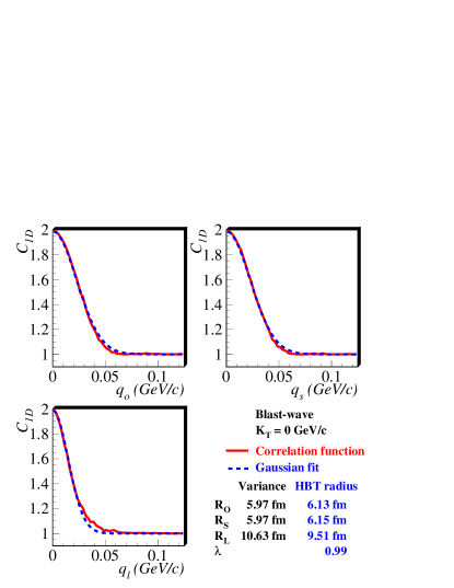
Figure 1: (Color online) One-dimensional slices of the three-dimensional correlation function along the “out”, “side”, and “long” directions, for pion pairs with $\bm{K}{\,=\,}0$, calculated from the blast-wave parameterization. For a given slice, the unplotted $q$-components equal 1.25 MeV/$c$ (i.e. the center of the first bin). The solid (red) curve is the calculated correlation function from Eq. (3), the dashed (blue) curve shows the same slice of the best 3D Gaussian fit (5), with “HBT parameters” calculated from the analytic expressions given in Sec. III.2.

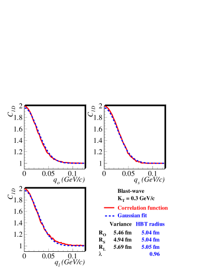
Figure 2: (Color online) Solid (red) curves show one-dimensional slices of the three-dimensional correlation function calculated with Eq. (3) from the blast-wave parameterization, for midrapidity pions with $K_{T}=0.3$ GeV/$c$. Dashed (red) curves show slices of the three-dimensional Gaussian form of Equation (5), with “HBT parameters” calculated from the analytic expressions given in Sec. III.2.

III.2 Three-dimensional Gaussian fit algorithm

Proceeding as in the previous subsection, we start from the general three-dimensional Gaussian ansatz (5) which can be written as

$$\ln\bigl{(}C(\bm{q}){-}1\bigr{)}=\ln\lambda-\left(q_{o}^{2}R_{o}^{2}{+}q_{s}^{2}R_{s}^{2}{+}q_{l}^{2}R_{l}^{2}\right).$$ (17)

If the correlation function $C\bigl{(}\bm{q}^{(k)}\bigr{)}$ in bin $k$ has error $\sigma_{k}$, the error on $\ln(C{-}1)$ is given as in (11) by

$$\sigma^{\prime}_{k}=\frac{\sigma_{k}}{C\bigl{(}\bm{q}^{(k)}\bigr{)}-1}\,.$$ (18)

We minimize

$$\chi^{2}=\sum_{k=1}^{N}\left[\frac{\ln{\bigl{(}C\bigl{(}\bm{q}^{(k)}\bigr{)}-1\bigr{)}}-\ln{\lambda}+{\displaystyle{\sum_{i=osl}}}\bigl{(}q_{i}^{(k)}\bigr{)}^{2}R^{2}_{i}}{\sigma^{\prime}_{k}}\right]^{2}$$ (19)

by setting

$$\frac{\partial\chi^{2}}{\partial\ln{\lambda}}=0\,,\qquad\frac{\partial\chi^{2}}{\partial R^{2}_{i}}=0\quad(i=o,s,l)\,.$$ (20)

This leads to a set of 4 coupled linear equations,

$$\sum_{\beta}T_{\alpha\beta}P_{\beta}=V_{\alpha}\,,$$ (21)

where $\alpha$ and $\beta$ take the values $\mathrm{\o},o,s,l$. The vectors appearing here are

$$P = \left(\ln{\lambda},R^{2}_{o},R^{2}_{s},R^{2}_{l}\right),$$ (22)

$$V_{\mathrm{\o}} = -\sum_{k=1}^{N}\frac{\ln{\bigl{(}C\bigl{(}\bm{q}^{(k)}\bigr{)}-1\bigr{)}}}{\left(\sigma_{k}^{\prime}\right)^{2}}\,,$$ (23)

$$V_{i} = +\sum_{k=1}^{N}\frac{\bigl{(}q_{i}^{(k)}\bigr{)}^{2}}{\left(\sigma_{k}^{\prime}\right)^{2}}\cdot\ln{\bigl{(}C\bigl{(}\bm{q}^{(k)}\bigr{)}-1\bigr{)}},\quad$$ (24)

while the symmetric $4\times 4$ matrix $T$ has components

$$T_{\mathrm{\o}\mathrm{\o}} = -\sum_{k=1}^{N}\frac{1}{\left(\sigma_{k}^{\prime}\right)^{2}}\,,$$

$$T_{\mathrm{\o}i} = +\sum_{k=1}^{N}\frac{\bigl{(}q_{i}^{(k)}\bigr{)}^{2}}{\left(\sigma_{k}^{\prime}\right)^{2}}\,,$$ (25)

$$T_{ij} = -\sum_{k=1}^{N}\frac{\bigl{(}q_{i}^{(k)}\bigr{)}^{2}\,\bigl{(}q_{j}^{(k)}\bigr{)}^{2}}{\left(\sigma_{k}^{\prime}\right)^{2}}\,.$$

In Equations (24) and (III.2) $i,j{\,=\,}{o,s,l}$ as usual. Note the correspondences $V_{\alpha}\leftrightarrow X_{n,i}$ and $T_{\alpha\beta}\leftrightarrow Y_{n,i}$ between the 3D and 1D cases.

The set of linear equations (21) is easily solved algebraically by diagonalizing the matrix $T_{\alpha\beta}$.

IV Application to blast-wave model

Many variants of “hydrodynamically-inspired” models of freeze-out have recently been used to calculate spatial RMS variances which then were compared to experimental HBT radii. A recent example is reported in reference Retiere:2003kf . The model itself is very simplistic and ignores, for example, resonance decay contributions which may be important Wiedemann:1996ig . We ignore such issues with the model itself and simply use it here to discuss differences between RMS variances and Gaussian HBT radii.

We use “realistic” model parameters which best describe the data Adams:2004yc . Specifically, we take $R{\,=\,}13.3$ fm for the source radius, $T{\,=\,}97$ MeV for the temperature, $\rho_{0}{\,=\,}1.03$ for the maximum transverse flow rapidity, $\tau{\,=\,}9$ fm/c for the average freeze-out time, and $\Delta\tau{\,=\,}2.83$ fm/c for the emission duration (see Retiere:2003kf for details).

IV.1 Correlation functions and analytic fits: results

Equation (12) of Retiere:2003kf gives the functional form for the single-pion emission function in the blast-wave model. Using this for $S(\bm{K},x)$, we calculate the correlation function for pion pairs with longitudinal pair momentum $K_{L}{\,=\,}0$, using a Monte Carlo technique to numerically perform the integrals in Eq. (3).

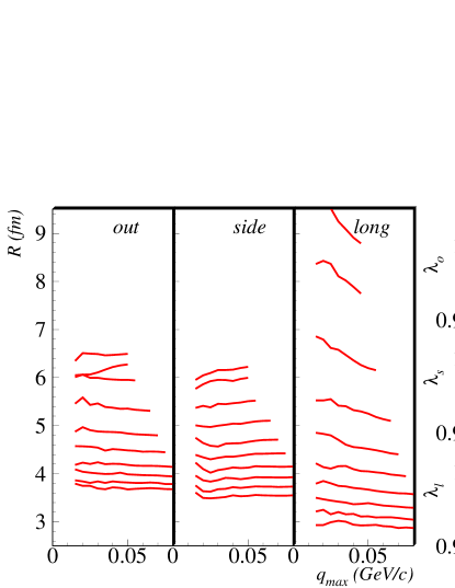
Figure 3: (Color online) From the blast-wave parameterization, one-dimensional HBT fit parameters $R_{\mathrm{1D},i}$ and $\lambda_{\mathrm{1D},i}$ are calculated with Eqs. (13,14) and plotted as a function of the maximum allowed value of any $q$-component; see text for details. Each curve corresponds to one of ten values of $K_{T}$: 0.0, 0.1, 0.2, …, 0.9 GeV/$c$. Curves corresponding to high $K_{T}$ are at low (high) values of $R_{\mathrm{1D},i}$ ($\lambda_{\mathrm{1D},i}$).

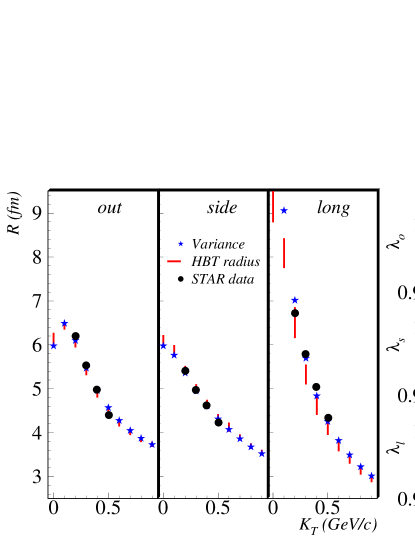
Figure 4: (Color online) One-dimensional HBT fit parameters $R_{\mathrm{1D},i}$ and $\lambda_{\mathrm{1D},i}$ as a function of $K_{T}$, calculated from the blast-wave parametrization with Eqs. (13,14). For a given $K_{T}$, the vertical red line represents the variation with fit range (see Figure 3). Blue stars represent the corresponding radius parameters calculated from the RMS variances using Eq. (II). Black circles show STAR data Adams:2004yc , with error bars removed for clarity.

As with experimental data, the correlation function is evaluated in finite-sized three-dimensional bins in $(q_{o},q_{s},q_{l})$ of width 2.5 MeV/$c$ in each direction. One-dimensional slices of the correlation function in the “out”, “side”, and “long” directions are shown in Figures 1 and 2, for midrapidity pion pairs with $K_{T}{\,=\,}0$ and $K_{T}{\,=\,}0.3$ GeV/$c$, respectively.

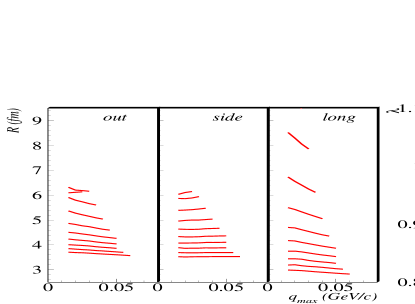
Figure 5: (Color online) From the blast-wave parameterization, three-dimensional HBT fit parameters $R_{i}$ and $\lambda$ are calculated with Eqs. (21) and plotted as a function of the maximum allowed value of any $q$-component; see text for details. Each curve corresponds to one of ten values of $K_{T}$: 0.0, 0.1, 0.2, …, 0.9 GeV/$c$. Curves corresponding to high $K_{T}$ are at low (high) values of $R_{i}$ ($\lambda$). The $R_{l}$ curve for $K_{T}{\,=\,}0$ falls above the plotting range.

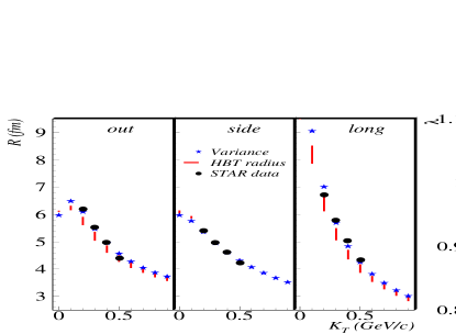
Figure 6: (Color online) Three-dimensional HBT fit parameters $R_{\mathrm{1D},i}$ and $\lambda_{\mathrm{1D},i}$ as a function of $K_{T}$, calculated from the blast-wave parametrization with Eqs. (21). For a given $K_{T}$, the vertical red line represents the variation with fit range (see Figure 5). Blue stars represent the corresponding radius parameters calculated from the RMS variances using Eq. (II). Black circles show STAR data Adams:2004yc , with error bars removed for clarity.

The slices of the correlation functions appear quite Gaussian, and they are tracked well by the three-dimensional Gaussian fit; the fitted correlation strength $\lambda$ is very close to 1. The radius parameters calculated from the RMS variances (II) agree quite well with the HBT radii extracted from the three-dimensional Gaussian fit by solving Eqs. (21); both sets are given in the Figures. Upon closer inspection one notices, however, that the fitted outward and longitudinal radii, $R_{o}$ and especially $R_{l}$, tend to be systematically smaller than those extracted from the spatial RMS variances; the opposite is true for the sideward radii $R_{s}$ for which the RMS variances give slightly smaller values than the Gaussian fit. While these differences are small for the blast-wave model parameterization (at least with the “realistic” parameters studied here), they will be significantly larger (with the same basic tendencies as found here) for the hydrodynamic model source studied in Sec. V.

The Gaussian fit parameters given in Figs. 1 and 2 correspond to using the largest possible $\bm{q}$-range in the sums over $k$ in Eqs. (24,III.2), discarding only those data points for which $C$ is so close to 1 that the Monte Carlo integration sometimes yields negative values for $C{-}1$. Due to small but noticeable deviations of the correlation function from a pure Gaussian, the Gaussian fit parameters depend on the number of data points used. We study this sensitivity to the fit range in the following subsection.

IV.2 Fit-range study

Since no measured correlation function is ever perfectly Gaussian, experimentalists typically perform so-called “fit range studies.” Here, the measured correlation function is fitted with the Gaussian form (5), using data points in a restricted range of $\bm{q}$. With correlation functions in the one-dimensional quantity $Q_{\mathrm{inv}}$ it is common to study the variation of fit parameters as the first few (lowest-$Q_{\mathrm{inv}}$) data points are left out of the fit. This is because statistical fluctuations in these bins may be quite large, and due to the visible non-Gaussian nature of the measured correlation function there. Three-dimensional correlation functions do not suffer from these issues, and so usually the experimentalist includes all data points with $|q_{i}|{\,<\,}q_{\mathrm{max}}$ and studies variations of the fit parameters as $q_{\mathrm{max}}$ is varied; any such variations are typically folded into systematic errors on the HBT radii.

Here, we follow the experimentalists’ approach. Using the correlation function generated from the blast-wave model, we calculate HBT parameters from 1D and 3D Gaussian fits as discussed in Sections III.1 and III.2, restricting the $k$-sums in Eqs. (15), (16), (24), and (III.2) to include only those data points where all three $q$-components have magnitudes less than $q_{\mathrm{max}}$ fn3 . Thus, we will not calculate unique HBT radii, but a finite range for each fit parameter.

For various values of $K_{T}$, Figure 3 shows the evolution of the 1D radii with $q_{\mathrm{max}}$. Except for $R_{l}$ at low $K_{T}$, the parameter variation with fit range is quite mild, corresponding to a small “non-Gaussian systematic error” on the radii. In Figure 4 the range of this variation, indicated by vertical lines, is plotted as a function of $K_{T}$. Consistent with the theorem Wiedemann:1999qn that the spatial RMS variances (II) of the source control the curvature of the correlator $C(\bm{q})$ at $\bm{q}{\,=\,}0$, the blue stars in Fig. 4 coincide with the $q_{\mathrm{max}}{\,\to\,}0$ limit of the fitted 1D radii. The largest fit-range variations, indicating the biggest non-Gaussian effects in the correlator, are seen at small pair momentum $K_{T}$. The fit-range sensitivity is most pronounced for $R_{l}$ (where at low $K_{T}$ it can exceed 0.5 fm) but almost negligible for $R_{o}$ and $R_{s}$. In short, the 1D Gaussian fits to the two transverse projections of the correlation function give length scales consistent with the spatial RMS variances of the source distribution, but non-Gaussian features along the longitudinal projection cause the RMS variances to overestimate the longitudinal 1D HBT radius $R_{l}$ by up to 0.5 fm at low $K_{T}$ if a reasonable fit range $q_{\mathrm{max}}$ is used to extract the latter. This discrepancy is significantly larger than the combined statistical and systematic error on the experimental value for $R_{l}$ Adams:2004yc .

Figures 5 and 6 show the same study for the three-dimensional Gaussian fits. For reasons explained in Sec. III.1, the non-Gaussian effects in a unified 3D Gaussian fit are expected to differ from those in 1D fits. Indeed, in the unified 3D fit non-Gaussian influences also appear in $R_{o}$, and both $R_{o}$ and $R_{l}$ now show fit-range variations which exceed the combined statistical and systematic errors of the data Adams:2004yc . The largest fit-range sensitivity is still seen in the longitudinal direction. In Ref. Retiere:2003kf the blast-wave model parameters were determined by comparing RMS variances with the measured HBT radii (see Figs. 4 and 6), using the experimental errors on the latter to extract error estimates for the model parameters. The results presented here suggest that if the authors had instead compared the measured data with HBT radii extracted from a 3D Gaussian fit to the calculated correlation function, they would have found somewhat different model parameters whose mean values in some cases might even have fallen outside the likely parameter range quoted in Table II of Ref. Retiere:2003kf . In particular, such an “apples-to-apples” comparison may allow for somewhat larger fireball lifetimes $\tau$ and/or emission durations $\Delta\tau$ than quoted in Ref. Retiere:2003kf . While such an improved blast-wave model fit is numerically expensive and outside the scope of the present paper, it may be a worthwhile future project.

V HBT radii from hydrodynamics

Non-viscous (“ideal”) hydrodynamical calculations have successfully reproduced differential momentum spectra (at least perpendicular to the beam direction) at RHIC, including their anisotropies in non-central collisions and the dependence of these anisotropies on the masses of the emitted hadrons Kolb:2003dz . As in the blast-wave model calculations, very strong collective flow is a critical ingredient to reproduce the data. (Of course, in the blast-wave parameterization such flow is put in by hand while it arises naturally in the hydrodynamical model.)

Most (but not all Hirano:2001yi ; Hirano:2002ds ; Morita:2002av ; Morita:2003mj ) hydrodynamic predictions of HBT radius parameters have been based on calculations of the spatial RMS variances from the hydrodynamically generated emission function, using Eqs. (II) Kolb:2003dz ; Heinz:2002un . In spite of the hydrodynamic model’s impressive success in describing hadron spectra, these predictions of HBT radii were a failure: The calculated longitudinal radii $R_{l}$ were too large (although this problem was less severe in Hirano and Tsuda’s work Hirano:2002ds ), while the predicted sideward radius $R_{s}$ was too small, and both $R_{s}$ and $R_{o}$ showed much less dependence on $K_{T}$ in theory than seen in the data. This, together with similar failures by other dynamical models (see Lisa:2005dd for a review), has become known as the “RHIC HBT Puzzle”.

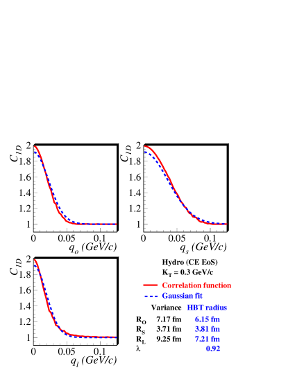
Figure 7: (Color online) Solid (red) curves show one-dimensional slices of the three-dimensional correlation function calculated with Eq. (3) from the hydrodynamic model with CE Equation of State, for midrapidity pions with $K_{T}=0.3$ GeV/$c$. Dashed (red) curves show slices of the three-dimensional Gaussian form of Equation (5), with “HBT parameters” calculated from the analytic expressions given in Sec. III.2.

Various possibilities to explain and correct this failure have been suggested. They include a more realistic modeling of the final freeze-out stage Soff:2000eh , exploration of fluctuations in the initial state and ambiguities in the hydrodynamic decoupling criterion Socolowski:2004hw , viscous effects due to incomplete thermalization (i.e. inapplicability of ideal fluid dynamics) Teaney:2003pb , different (more Landau-type) initial conditions leading to strong longitudinal hydrodynamic acceleration Renk:2004yv , and the use of more realistic or different equations of state (EoS) for the expanding matter Huovinen:2005gy . None of these suggestions, individually or in combination, has been convincingly shown to be able to solve the HBT puzzle. Motivated by the blast-wave study in the preceding section, we therefore explore here one further possibility: that previous comparisons of the data with hydrodynamic models might have been misleading since the RMS variances from hydro-generated sources differ significantly from HBT radii extracted from a Gaussian parameterization of the correlation function. Indications that this is indeed the case have already emerged from the work on 1D projections of Hirano and Tsuda Hirano:2002ds and Kolb fn1 , and with our new analytic 3D Gaussian fit algorithm we can improve on their analysis and study this question in more detail.

For our study of HBT radii from the hydrodynamic model we use two different sets of emission functions, obtained from running the hydrodynamic code with two different equations of state (EoS). Both EoS describe the quark-gluon plasma (QGP) as a free gas of massless particles, but they differ in their treatment of the late hadronic stage when the fireball has cooled below the critical temperature $T_{c}{\,\approx\,}165$ MeV for hadronization. The “CE EoS” Sollfrank:1996hd ; Kolb:2000sd assumes that the hadron resonance gas remains not only in thermal, but also in chemical equilibrium until final kinetic freeze-out. This fails to reproduce the observed hadron yields which correspond to chemical equilibrium at a temperature of about 170 MeV Braun-Munzinger:2001ip . The “NCE EoS” Hirano:2002ds ; Kolb:2002ve ; Teaney:2002aj takes the immediate decoupling of hadron abundances at $T_{c}$ into account by introducing non-equilibrium chemical potentials for each hadron species which ensure that the particle yields are held fixed as the temperature and density continue to decrease. While the CE EoS was used for the hydrodynamic model predictions made for RHIC before the accelerator turned on and the hadron abundances were measured, the NCE EoS is more realistic and has been used in most hydrodynamic studies since 2002. We here explore emission functions obtained with either EoS.

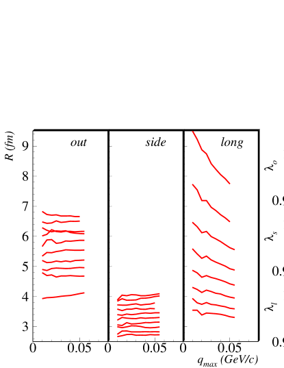
Figure 13: (Color online) From the hydro model with NCE EoS, one-dimensional HBT fit parameters $R_{\mathrm{1D},i}$ and $\lambda_{\mathrm{1D},i}$ are calculated with Eqs. (13,14) and plotted as a function of the maximum allowed value of any $q$-component; see text for details. Each curve corresponds to one of ten values of $K_{T}$: 0.0, 0.1, 0.2, …, 0.9 GeV/$c$. Curves corresponding to high $K_{T}$ are at low (high) values of $R_{\mathrm{1D},i}$ ($\lambda_{\mathrm{1D},i}$). The $R_{l}$ curves for $K_{T}{\,\leq\,}0.1$ GeV/$c$ fall above the plotting range.

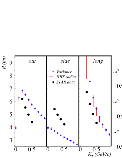
Figure 14: (Color online) One-dimensional HBT fit parameters $R_{\mathrm{1D},i}$ and $\lambda_{\mathrm{1D},i}$ as a function of $K_{T}$, calculated from the hydrodynamic model using NCE EoS with Eqs. (13,14). For a given $K_{T}$, the vertical red line represents the variation with fit range (see Figure 13). Blue stars represent the corresponding radius parameters calculated from the RMS variances using Eq. (II). Black circles show STAR data Adams:2004yc , with error bars removed for clarity.

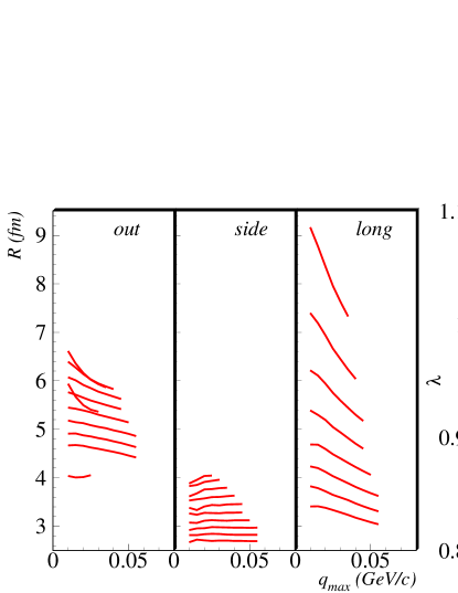
Figure 15: (Color online) From the hydrodynamic model with NCE EoS, three-dimensional HBT fit parameters $R_{i}$ and $\lambda$ are calculated with Eqs. (21) and plotted as a function of the maximum allowed value of any $q$-component; see text for details. Each curve corresponds to one of ten values of $K_{T}$: 0.0, 0.1, 0.2, …, 0.9 GeV/$c$. Curves corresponding to high $K_{T}$ are at low (high) values of $R_{i}$ ($\lambda$). The $R_{l}$ curves for $K_{T}{\,\leq\,}0.1$ GeV/$c$ fall above the plotting range.

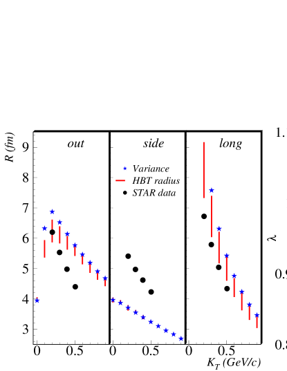
Figure 16: (Color online) Three-dimensional HBT fit parameters $R_{\mathrm{1D},i}$ and $\lambda_{\mathrm{1D},i}$ as a function of $K_{T}$, calculated from the hydrodynamic model using NCE EoS with Eqs. (21). For a given $K_{T}$, the vertical red line represents the variation with fit range (see Figure 15). Blue stars represent the corresponding radius parameters calculated from the RMS variances using Eq. (II). Black circles show STAR data Adams:2004yc , with error bars removed for clarity.

Figures 7-11 present 1D projections and 1D and 3D fit results, analogous to those from the previous section, for the emission function from hydrodynamic calculations using the CE EoS. Figures 12-16 show the same for the NCE EoS. Several observations are in order.

As is apparent from Figures 7 and 12, the best 3D Gaussian fits do not fully reproduce the correlation function, even though the correlation function projections themselves appear rather Gaussian. Clearly, aspects of the correlation function not apparent in the one-dimensional projections are partially driving the 3D fit. Further, it is interesting to note that, while the projections in the “side” direction appear the worst reproduced by the fit, the greatest discrepancy between RMS variances and HBT radii are in fact in the “out” and “long” directions (c.f. Figures 11 and 16). Both of these points emphasize that the three-dimensional correlator can contain important information which does not appear in its one-dimensional projections, and thus in the one-dimensional fits. Particularly important in this case are strong non-Gaussian features in the longitudinal direction which cause a significant suppression of the correlation strength parameter $\lambda$ of the 3D Gaussian fit. This in turn creates the appearance of a “bad fit” in the sideward direction even though the 1D sideward projection looks quite Gaussian itself.

One draws the same conclusion by examining the fit-range systematics. As mentioned, non-Gaussian effects generate a variation of the HBT parameters with $q_{\mathrm{max}}$. As seen in Figures 8 and 13, fits in the “out” and “side” directions produce 1D radii and directional $\lambda_{i}$ parameters which vary very little with $q_{\mathrm{max}}$; strong fit-range sensitivity is only seen in the “long” direction where the 1D projection deviates most strongly from a Gaussian form. In the three-dimensional fits, on the other hand (c.f. Figures 10 and 15), the strong non-Gaussian features in the $q_{l}$ direction now affect all four fit parameters, generating strong fit-range sensitivities also for $R_{o}$ and $\lambda$.

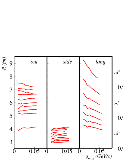
Figure 8: (Color online) From the hydrodynamic model with CE EoS, one-dimensional HBT fit parameters $R_{\mathrm{1D},i}$ and $\lambda_{\mathrm{1D},i}$ are calculated with Eqs. (13,14) and plotted as a function of the maximum allowed value of any $q$-component; see text for details. Each curve corresponds to one of ten values of $K_{T}$: 0.0, 0.1, 0.2, …, 0.9 GeV/$c$. Curves corresponding to high $K_{T}$ are at low (high) values of $R_{\mathrm{1D},i}$ ($\lambda_{\mathrm{1D},i}$). The $R_{l}$ curves for $K_{T}{\,\leq\,}0.2$ GeV/$c$ fall above the plotting range.

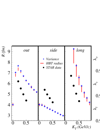
Figure 9: (Color online) One-dimensional HBT fit parameters $R_{\mathrm{1D},i}$ and $\lambda_{\mathrm{1D},i}$ as a function of $K_{T}$, calculated from the hydrodynamic model using CE EoS with Eqs. (13,14). For a given $K_{T}$, the vertical red line represents the variation with fit range (see Figure 8). Blue stars represent the corresponding radius parameters calculated from the RMS variances using Eq. (II). Black circles show STAR data Adams:2004yc , with error bars removed for clarity.

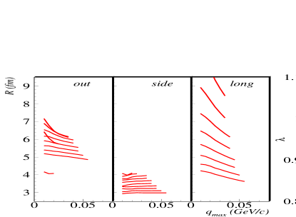
Figure 10: (Color online) From the hydrodynamic model with CE EoS, three-dimensional HBT fit parameters $R_{i}$ and $\lambda$ are calculated with Eqs. (21) and plotted as a function of the maximum allowed value of any $q$-component; see text for details. Each curve corresponds to one of ten values of $K_{T}$: 0.0, 0.1, 0.2, …, 0.9 GeV/$c$. Curves corresponding to high $K_{T}$ are at low (high) values of $R_{i}$ ($\lambda$). The $R_{l}$ curves for $K_{T}{\,\leq\,}0.1$ GeV/$c$ fall above the plotting range.

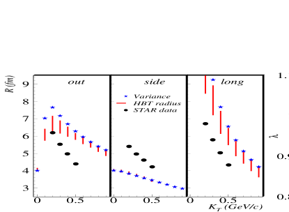
Figure 11: (Color online) Three-dimensional HBT fit parameters $R_{\mathrm{1D},i}$ and $\lambda_{\mathrm{1D},i}$ as a function of $K_{T}$, calculated from the hydrodynamic model using CE EoS with Eqs. (21). For a given $K_{T}$, the vertical red line represents the variation with fit range (see Figure 10). Blue stars represent the corresponding radius parameters calculated from the RMS variances using Eq. (II). Black circles show STAR data Adams:2004yc , with error bars removed for clarity.

There may (and in general will) be other properties of the three-dimensional correlation function to which the 1D projections and their Gaussian fits are not sensitive but which affect the 3D Gaussian fit. The extracted values for $R_{o}$ and $R_{s}$ thus in general depend significantly on the detailed conditions under which the Gaussian fit is performed. Hence, a meaningful and accurate comparison between models and experimental data requires that the Gaussian fit to the theoretical correlation functions is done under similar conditions and constraints (e.g. fit range) as the in experiment.

Figure 12: (Color online) Solid (red) curves show one-dimensional slices of the three-dimensional correlation function calculated with Eq. (3) from the hydrodynamic model with NCE Equation of State, for midrapidity pions with $K_{T}=0.3$ GeV/$c$. Dashed (red) curves show slices of the three-dimensional Gaussian form of Equation (5), with “HBT parameters” calculated from the analytic expressions given in Sec. III.2.

VI Discussion and Conclusions

Let us close with some general observations and summarize our conclusions.

Except inasmuch as it couples HBT radii in a 3D fit, we have not focused here on the $\lambda$ parameter, since comparison to measurements of $\lambda$ is significantly complicated by experimental artifacts Lisa:2005dd . This is also the reason why tests of consistency between different experiments generally compare HBT radii, not $\lambda$. In all of the idealized calculations presented in this report $C(|\bm{q}|{=}0){\,=\,}2$, so a purely Gaussian correlation function (generated by a purely Gaussian source) would yield $\lambda{\,=\,}1$, with no fit-range systematics. Indeed, we find that $\lim_{q_{\mathrm{max}}\rightarrow 0}\lambda{\,=\,}1$ (see e.g. Figure 10) as expected, but that its value declines as more bins are included in the fit. In experimental data, several factors cause $\lambda$ to fall below its nominal value of unity. Our calculations confirm the generally held folklore that non-Gaussian effects may be important to understanding $\lambda$.

Of more fundamental interest are the characteristic length scales of the emission region. We have seen that RMS variances of model-calculated source functions, which are frequently compared to experimentally extracted HBT radii, may systematically differ from “fitted” HBT radii which characterize the shape of the correlation function from the same model. Since the latter quantity provides the best “apples-to-apples” comparison to published experimental data, this can be an important observation.

Previous attempts Wiedemann:1996ig ; fn1 ; Hirano:2002ds to estimate the effect in hydrodynamical calculations have focused on numerical fits to several one-dimensional projections of the calculated correlation function. We here presented an analytic method to extract these “1D HBT radii” from the projections, and further generalized it to the full three-dimensional case. The 1D projections represent a set of zero measure of the full three-dimensional correlation function and, as we have seen, may not be sensitive to important three-dimensional information. This information influences the unified three-dimensional fit to the correlation function. Since the unified 3D fit most closely mimics the procedure of experimentalists, these effects are relevant for comparisons between models and data.

The magnitude of these effects are model dependent. The non-Gaussian nature of emission regions in the blast-wave parameterization has been noted before Retiere:2003kf . It was shown here to generate only minor deviations from Gaussian behaviour in the transverse projections of the correlation function, but the longitudinal projection shows significant non-Gaussian features. In a unified 3D Gaussian fit, non-Gaussian features were seen to generate fit-range sensitivities for all four fit-parameters, leading to significant downward shifts of both $R_{l}$ and $R_{o}$, especially at low $K_{T}$, relative to predictions based on the spatial RMS variances of the blast-wave source.

These tendencies were found to be even more strongly exhibited by the HBT radii extracted from hydrodynamic model sources. The differences between HBT radii extracted from 3D Gaussian fits of the correlator and the values (II) calculated from the spatial RMS variances are quite significant and thus relevant in considerations of the “RHIC HBT puzzle”. In particular, for both equations of state considered here, the HBT radii in the “out” and “long” directions are significantly lower (and closer to the data) than the corresponding RMS variances which have been the basis of many “puzzle” discussions (c.f. Figures 11 and 16). As in the blast-wave model, these 3D Gaussian fit effects seem to be mostly driven by strong non-Gaussian features in the longitudinal projection of the correlator. Combining improvements of using the NCE EoS and the use of HBT radii instead of RMS variances brings the hydrodynamic calculations for the longitudinal radius $R_{l}$ into fair agreement with the data over the entire measured $K_{T}$ range. A significant improvement is also seen in the outward direction, but it is mostly concentrated at low $K_{T}$, and hence the disagreement between the rather steep $K_{T}$-dependence of the measured $R_{o}$ radii and the much flatter $K_{T}$-dependence of the theoretical results is getting worse. The fitted sideward radii $R_{s}$ show practically no deviation from the corresponding RMS variances, and the well-known Heinz:2002un problem that the hydrodynamically predicted values are significantly smaller and show much less $K_{T}$-dependence than the data is not alleviated by our improved comparison between theory and data.

While the results presented here can not offer a resolution of all aspects of the “RHIC HBT Puzzle”, they refocus our perception of where the most severe problems are located. The strong non-Gaussian effects in $q_{l}$ direction and the resulting large downward shift of the fitted longitudinal radii (as compared to the corresponding RMS variances) largely eliminate the discrepancies between hydrodynamically predicted and measured $R_{l}$ values. A number of authors have interpreted the smallness of the measured $R_{l}$ values as evidence for a short fireball lifetime $\tau_{f}{\,<\,}10$ fm/$c$, inconsistent with the $O(15\,\mathrm{fm}/c)$ lifetimes predicted Kolb:2003dz by the hydrodynamic model. The analysis presented here resolves this problem. On the other hand, even when using the properly extracted Gaussian fit values for $R_{s}$ and $R_{o}$ and after taking into account the resulting decrease of $R_{o}$ at low $K_{T}$, the theoretically predicted ratio $R_{o}/R_{s}$ is still significantly larger than 1 over the entire measured $K_{T}$ interval, in contradiction to the data. Furthermore, the decline of both $R_{o}$ and $R_{s}$ with increasing pair momentum is still much too weak in the model, in spite of the large transverse flow generated by the hydrodynamic expansion. These aspects of the HBT Puzzle remain serious and must be addressed by other theoretical improvements.

Finally, one should remember that the raw experimental correlation functions hardly ever appear very Gaussian, due to additional distortions by the final state Coulomb interactions between the two charged particles. Modern methods of extracting the HBT radii from the measured correlator include these Coulomb effects selfconsistently in the fit function Lisa:2005dd , leading to more complicated (numerical) fit algorithms than the analytical one presented in Section III. Nonetheless, the measured HBT radii extracted from such self-consistent 3D fits are affected by non-Gaussian structures in the underlying Bose-Einstein correlations in much the same way as discussed here for the simpler case of non-interacting particles. Thus, while Coulomb interactions should be included in future studies, our analysis should provide a good estimate of the direction and magnitude of non-Gaussian effects in blast-wave and hydrodynamical models, and it points out the importance of such effects in the comparison of theory to experiment.

References

- (1) M. A. Lisa, S. Pratt, R. Soltz and U. Wiedemann, Ann. Rev. Nucl. Part. Sci. 55 (2005) 357 [arXiv:nucl-ex/0505014].
- (2) S. V. Akkelin and Y. M. Sinyukov, Phys. Lett. B 356, 525 (1995).
- (3) U. A. Wiedemann and U. Heinz, Phys. Rev. C 56, 610 (1997). [arXiv:nucl-th/9610043].
- (4) J. Adams et al. [STAR Collaboration], Phys. Rev. C 71, 044906 (2005). [arXiv:nucl-ex/0411036].
- (5) D. A. Brown and P. Danielewicz, Phys. Lett. B 398, 252 (1997). [arXiv:nucl-th/9701010].
- (6) D. A. Brown, P. Danielewicz, M. Heffner and R. Soltz, Acta Phys. Hung. A24 (2005) 111 [nucl-th/0404067].
- (7) D. A. Brown, A. Enokizono, M. Heffner, R. Soltz, P. Danielewicz and S. Pratt, Phys. Rev. C 72 (2005) 054902. [arXiv:nucl-th/0507015].
- (8) U. A. Wiedemann and U. Heinz, Phys. Rept. 319, 145 (1999). [arXiv:nucl-th/9901094].
- (9) P. F. Kolb and U. Heinz, in Quark-Gluon Plasma 3, edited by R.C. Hwa and X.-N. Wang (World Scientific, Singapore, 2004), p. 634 [nucl-th/0305084].
- (10) U. Heinz and P. F. Kolb, in Proceedings of the 18th Winter Workshop on Nuclear Dynamics, edited by R. Bellwied, J. Harris and W. Bauer (EP Systema, Debrecen, Hungary, 2002), p. 205 [hep-ph/0204061].
- (11) T. Hirano, K. Morita, S. Muroya and C. Nonaka, Phys. Rev. C 65, 061902 (2002) [arXiv:nucl-th/0110009].
- (12) K. Morita, S. Muroya, C. Nonaka and T. Hirano, Phys. Rev. C 66, 054904 (2002) [arXiv:nucl-th/0205040].
- (13) K. Morita and S. Muroya, Prog. Theor. Phys. 111, 93 (2004) [arXiv:nucl-th/0307026].
- (14) P. F. Kolb, private communication (May 2002).
- (15) T. Hirano and K. Tsuda, Phys. Rev. C 66, 054905 (2002). [arXiv:nucl-th/0205043].
- (16) D. Molnar and M. Gyulassy, Phys. Rev. Lett. 92, 052301 (2004). [arXiv:nucl-th/0211017].
- (17) D. Hardtke and S. A. Voloshin, Phys. Rev. C 61, 024905 (2000) [arXiv:nucl-th/9906033].
- (18) S. Soff, S. A. Bass, D. H. Hardtke and S. Y. Panitkin, Phys. Rev. Lett. 88, 072301 (2002) [arXiv:nucl-th/0109055].
- (19) Z. w. Lin, C. M. Ko and S. Pal, Phys. Rev. Lett. 89, 152301 (2002). [arXiv:nucl-th/0204054].
- (20) U. A. Wiedemann and U. Heinz, Phys. Rev. C 56, 3265 (1997). [arXiv:nucl-th/9611031].
- (21) A. Kisiel, W. Florkowski, W. Broniowski and J. Pluta, arXiv:nucl-th/0602039.
- (22) F. Retiere and M. A. Lisa, Phys. Rev. C 70, 044907 (2004). [arXiv:nucl-th/0312024].
- (23) S. Pratt, Phys. Rev. Lett. 53, 1219 (1984).
- (24) Note that for one-dimensional correlations measured in , as opposed to one-dimensional slices of the three-dimensional correlator, phase-space considerations usually produce larger uncertainties at small .
- (25) U. Heinz, A. Hummel, M. A. Lisa and U. A. Wiedemann, Phys. Rev. C 66, 044903 (2002). [arXiv:nucl-th/0207003].
- (26) When the HBT radii are large (e.g. at low ), the correlator approaches unity quickly with increasing , and the quantity becomes numerically unwieldy; in these cases only small values of are used.
- (27) S. Soff, S. A. Bass and A. Dumitru, Phys. Rev. Lett. 86, 3981 (2001). [arXiv:nucl-th/0012085].
- (28) O. J. Socolowski, F. Grassi, Y. Hama and T. Kodama, Phys. Rev. Lett. 93, 182301 (2004). [arXiv:hep-ph/0405181].
- (29) D. Teaney, Phys. Rev. C 68, 034913 (2003).
- (30) T. Renk, Phys. Rev. C 70, 021903 (2004). [arXiv:hep-ph/0404140].
- (31) P. Huovinen, Nucl. Phys. A 761, 296 (2005). [arXiv:nucl-th/0505036].
- (32) J. Sollfrank et al. Phys. Rev. C 55, 392 (1997). [arXiv:nucl-th/9607029].
- (33) P. F. Kolb, J. Sollfrank and U. Heinz, Phys. Rev. C 62, 054909 (2000). [arXiv:hep-ph/0006129].
- (34) P. Braun-Munzinger, D. Magestro, K. Redlich and J. Stachel, Phys. Lett. B 518, 41 (2001). [arXiv:hep-ph/0105229].
- (35) P. F. Kolb and R. Rapp, Phys. Rev. C 67, 044903 (2003). [arXiv:hep-ph/0210222].
- (36) D. Teaney, nucl-th/0204023.