Abstract

We discuss the phase diagram of moderately dense, locally neutral three-flavor quark matter using the framework of an effective model of quantum chromodynamics with a local interaction. The phase diagrams in the plane of temperature and quark chemical potential as well as in the plane of temperature and lepton-number chemical potential are discussed.

Chapter 0 PHASE DIAGRAM OF NEUTRAL QUARK MATTER AT MODERATE DENSITIES

1 Introduction

Theoretical studies suggest that baryon matter at sufficiently high density and sufficiently low temperature is a color superconductor. (For reviews on color superconductivity see, for example, Ref. reviews.) In nature, the highest densities of matter are reached in central regions of compact stars. There, the density might be as large as $10\rho_{0}$ where $\rho_{0}\approx 0.15$ fm^-3 is the saturation density. It is possible that baryonic matter is deconfined under such conditions and, perhaps, it is color-superconducting.

In compact stars, matter in the bulk is neutral with respect to the electric and color charges. Matter should also remain in $\beta$ equilibrium. Taking these constraints consistently into account may have a strong effect on the competition between different phases of deconfined quark matter at large baryon densities.[2, 3, 4, 5, 6]

The first attempts to obtain the phase diagram of dense, locally neutral three-flavor quark matter as a function of the strange quark mass, the quark chemical potential, and the temperature were made in Refs. SRP and phase-d. This was done within the framework of a Nambu–Jona-Lasinio (NJL) model. It was shown that, at zero temperature and small values of the strange quark mass, the ground state of matter corresponds to the color-flavor-locked (CFL) phase.[8, 9] At some critical value of the strange quark mass, this is replaced by the gapless CFL (gCFL) phase.[6] In addition, several other phases were found at nonzero temperature. For instance, it was shown that there should exist a metallic CFL (mCFL) phase, a so-called uSC phase,[10] as well as the standard two-flavor color-superconducting (2SC) phase[11, 12] and the gapless 2SC (g2SC) phase.[5]

In Ref. phase-d, the effect of the strange quark mass was incorporated only approximately through a shift of the chemical potential of strange quarks, $\mu_{s}\to\mu_{s}-m_{s}^{2}/(2\mu)$. While such an approach is certainly reliable at small values of the strange quark mass, it becomes uncontrollable with increasing the mass. The phase diagram of Ref. phase-d was further developed in Refs. phase-d1 and phase-d2 where the shift-approximation in dealing with the strange quark was not employed any more, although quark masses were still treated as free parameters, rather than dynamically generated quantities. In Refs. pd-mass and pd-nu the phase diagram of dense, locally neutral three-flavor quark matter was further improved by treating dynamically generated quark masses self-consistently. Some results within this approach at zero and nonzero temperatures were also obtained in Refs. SRP, kyoto, pd-other and kyoto2.

The results of Refs. pd-mass and pd-nu are presented here. Only locally neutral phases are considered. This excludes, for example, mixed[20] and crystalline[21] phases. Taking them into account requires a special treatment. We also discuss the effect of a nonzero neutrino (or, more precisely, lepton-number) chemical potential on the structure of the phase diagram.[16] This is expected to have a potential relevance for the physics of protoneutron stars where neutrinos are trapped during the first few seconds of the stellar evolution.

The effect of neutrino trapping on color-superconducting quark matter has been previously discussed in Ref. SRP. There it was found that a nonzero neutrino chemical potential favors the 2SC phase and disfavors the CFL phase. This is not unexpected because the neutrino chemical potential is related to the conserved lepton number in the system and therefore it also favors the presence of (negatively) charged leptons. This helps 2SC-type pairing because electrical neutrality in quark matter can be achieved without inducing a very large mismatch between the Fermi surfaces of up and down quarks. The CFL phase, on the other hand, is electrically and color neutral in the absence of charged leptons when $T=0$.[22] A nonzero neutrino chemical potential can only spoil CFL-type pairing.

A more systematic survey of the phase diagram in the space of temperature, quark and lepton-number chemical potentials was performed in Ref. pd-nu. In particular, this included the possibility of gapless phases, which have not been taken into account in Ref. SRP. While such phases are generally unstable at zero temperature,[23] this is not always the case at nonzero temperature.[24] Keeping this in mind, we shall merely localize the “problematic” regions in the phase diagram, where unconventional pairing is unavoidable. We shall refrain, however, from speculating on various possibilities for the true ground state (see, e.g., Refs. mix,cryst,spin-1,meson-cond,hong,gluonic), since these are still under debate.

In the application to protoneutron stars, it is of interest to cover a range of parameters that could provide a total lepton fraction in quark matter of up to about 0.4. This is the value of the lepton-to-baryon charge ratio in iron cores of progenitor stars. Because of the conservation of both lepton and baryon charges, this value is also close to the lepton fraction in protoneutron stars at early times, when the leptons did not have a chance to diffuse through dense matter and escape from the star.[29] In the model introduced in the next section, almost the whole range of possibilities will be covered by restricting the quark chemical potential to $\mu\lesssim 500~{}\mbox{MeV}$ and the neutrino chemical potential to $\mu_{\nu_{e}}\lesssim 400~{}\mbox{MeV}$.

2 Model

Let us start by introducing the effective model of QCD used in the analysis. This is a three-flavor quark model with a local NJL-type interaction, whose Lagrangian density is given by

$$\mathcal{L} = \bar{\psi}\,(i\not{\partial}-\hat{m}\,)\psi+G_{S}\sum_{a=0}^{8}\left[\left(\bar{\psi}\lambda_{a}\psi\right)^{2}+\left(\bar{\psi}i\gamma_{5}\lambda_{a}\psi\right)^{2}\right]$$ (1)

$$+ G_{D}\sum_{\gamma,c}\left[\bar{\psi}_{\alpha}^{a}i\gamma_{5}\epsilon^{\alpha\beta\gamma}\epsilon_{abc}(\psi_{C})_{\beta}^{b}\right]\left[(\bar{\psi}_{C})_{\rho}^{r}i\gamma_{5}\epsilon^{\rho\sigma\gamma}\epsilon_{rsc}\psi_{\sigma}^{s}\right]$$

$$- K\left\{\det_{f}\left[\bar{\psi}\left(1+\gamma_{5}\right)\psi\right]+\det_{f}\left[\bar{\psi}\left(1-\gamma_{5}\right)\psi\right]\right\}\;,$$

where the quark spinor field $\psi_{\alpha}^{a}$ carries color ($a=r,g,b$) and flavor ($\alpha=u,d,s$) indices. The matrix of quark current masses is given by $\hat{m}=\mbox{diag}_{f}(m_{u},m_{d},m_{s})$. Regarding other notations, $\lambda_{a}$ with $a=1,\ldots,8$ are the Gell-Mann matrices in flavor space, and $\lambda_{0}\equiv\sqrt{2/3}\,\mathbf{1}_{f}$. The charge conjugate spinors are defined as follows: $\psi_{C}=C\bar{\psi}^{T}$ and $\bar{\psi}_{C}=\psi^{T}C$, where $\bar{\psi}=\psi^{\dagger}\gamma^{0}$ is the Dirac conjugate spinor and $C=i\gamma^{2}\gamma^{0}$ is the charge conjugation matrix.

The model in Eq. (1) should be viewed as an effective model of strongly interacting matter that captures at least some key features of QCD dynamics. The Lagrangian density contains three different interaction terms which are chosen to respect the symmetries of QCD. Note that we include the ’t Hooft interaction whose strength is determined by the coupling constant $K$. This term breaks the $U(1)$ axial symmetry.

The term in the second line of Eq. (1) describes a scalar diquark interaction in the color antitriplet and flavor antitriplet channel. For symmetry reasons there should also be a pseudoscalar diquark interaction with the same coupling constant. This term would be important to describe Goldstone boson condensation in the CFL phase.[30]

We use the following set of model parameters:[31]

$$m_{u}=m_{d}=5.5~{}\mathrm{MeV},\quad m_{s}=140.7~{}\mathrm{MeV},$$ (2a)

$$G_{S}\Lambda^{2}=1.835,\qquad K\Lambda^{5}=12.36,\quad\Lambda=602.3~{}\mathrm{MeV}.$$ (2b)

After fixing the masses of the up and down quarks at equal values, $m_{u,d}=5.5~{}\mbox{MeV}$, the other four parameters are chosen to reproduce the following four observables of vacuum QCD: $m_{\pi}=135.0~{}\mbox{MeV}$, $m_{K}=497.7~{}\mbox{MeV}$, $m_{\eta^{\prime}}=957.8~{}\mbox{MeV}$, and $f_{\pi}=92.4~{}\mbox{MeV}$.[31] This parameter set gives $m_{\eta}=514.8~{}\mbox{MeV}$.

In Ref. RKH, the diquark coupling $G_{D}$ was not fixed by the fit of the meson spectrum in vacuum. In general, it is expected to be of the same order as the quark-antiquark coupling $G_{S}$. Here, we choose the coupling strength with $G_{D}=\frac{3}{4}G_{S}$ which follows from the Fierz identity.

The grand partition function, up to an irrelevant normalization constant, is given by

$$\mathcal{Z}\equiv e^{-\Omega V/T}=\int\mathcal{D}\bar{\psi}\mathcal{D}\psi\,e^{i\int_{X}\left(\mathcal{L}+\bar{\psi}\hat{\mu}\gamma^{0}\psi\right)}\;,$$ (3)

where $\Omega$ is the thermodynamic potential density, $V$ is the volume of the three-space, and $\hat{\mu}$ is a diagonal matrix of quark chemical potentials. In chemical equilibrium (which provides $\beta$ equilibrium as a special case), the nontrivial components of this matrix are extracted from the following relation:

$$\mu_{ab}^{\alpha\beta}=\left(\mu\delta^{\alpha\beta}+\mu_{Q}Q_{f}^{\alpha\beta}\right)\delta_{ab}+\left[\mu_{3}\left(T_{3}\right)_{ab}+\mu_{8}\left(T_{8}\right)_{ab}\right]\delta^{\alpha\beta}\;.$$ (4)

Here $\mu$ is the quark chemical potential (by definition, $\mu=\mu_{B}/3$ where $\mu_{B}$ is the baryon chemical potential), $\mu_{Q}$ is the chemical potential of electric charge, while $\mu_{3}$ and $\mu_{8}$ are color chemical potentials associated with two mutually commuting color charges of the $SU(3)_{c}$ gauge group, cf. Ref. BuSh. The explicit form of the electric charge matrix is $Q_{f}=\mbox{diag}_{f}(\frac{2}{3},-\frac{1}{3},-\frac{1}{3})$, and the explicit form of the color charge matrices is $T_{3}=\mbox{diag}_{c}(\frac{1}{2},-\frac{1}{2},0)$ and $\sqrt{3}T_{8}=\mbox{diag}_{c}(\frac{1}{2},\frac{1}{2},-1)$.

In order to calculate the mean-field thermodynamic potential at temperature $T$, we first linearize the interaction in the presence of the diquark condensates $\Delta_{c}\sim(\bar{\psi}_{C})_{\alpha}^{a}i\gamma_{5}\epsilon^{\alpha\beta c}\epsilon_{abc}\psi_{\beta}^{b}$ (no sum over $c$) and the quark-antiquark condensates $\sigma_{\alpha}\sim\bar{\psi}_{\alpha}^{a}\psi_{\alpha}^{a}$ (no sum over $\alpha$). Then, integrating out the quark fields and neglecting the fluctuations of composite order parameters, we arrive at the following expression for the thermodynamic potential:

$$\Omega = \Omega_{L}+\frac{1}{4G_{D}}\sum_{c=1}^{3}\left|\Delta_{c}\right|^{2}+2G_{S}\sum_{\alpha=1}^{3}\sigma_{\alpha}^{2}$$ (5)

$$- 4K\sigma_{u}\sigma_{d}\sigma_{s}-\frac{T}{2V}\sum_{K}\ln\det\frac{S^{-1}}{T}\;,$$

where we also added the contribution of leptons, $\Omega_{L}$, which will be specified later.

We should note that we have restricted ourselves to field contractions corresponding to the Hartree approximation. In a more complete treatment, among others, the ’t Hooft interaction term gives also rise to mixed contributions containing both diquark and quark-antiquark condensates, i.e., $\propto\sum_{\alpha=1}^{3}\sigma_{\alpha}|\Delta_{\alpha}|^{2}$.[33] In this study, we neglect such terms for simplicity. While their presence may change the results quantitatively, one does not expect them to modify the qualitative structure of the phase diagram.

In Eq. (5), $S^{-1}$ is the inverse full quark propagator in the Nambu-Gorkov representation,

$$S^{-1}=\left(\begin{array}[]{cc}[G_{0}^{+}]^{-1}&\Phi^{-}\\ \Phi^{+}&[G_{0}^{-}]^{-1}\end{array}\right)\;,$$ (6)

with the diagonal elements being the inverse Dirac propagators of quarks and of charge-conjugate quarks,

$$[G_{0}^{\pm}]^{-1}=\gamma^{\mu}K_{\mu}\pm\hat{\mu}\gamma_{0}-\hat{M}\;,$$ (7)

where $K^{\mu}=(k_{0},\mathbf{k})$ denotes the four-momentum of the quark. At nonzero temperature, we use the Matsubara imaginary time formalism. Therefore, the energy $k_{0}$ is replaced with $-i\omega_{n}$ where $\omega_{n}\equiv(2n+1)\pi T$ are the fermionic Matsubara frequencies. Accordingly, the sum over $K$ in Eq. (5) should be interpreted as a sum over integer $n$ and an integral over the three-momentum $\mathbf{k}$.

The constituent quark mass matrix $\hat{M}=\mbox{diag}_{f}(M_{u},M_{d},M_{s})$ is defined by

$$M_{\alpha}=m_{\alpha}-4G_{S}\sigma_{\alpha}+2K\sigma_{\beta}\sigma_{\gamma}\;,$$ (8)

where $\sigma_{\alpha}$ are the quark-antiquark condensates, and the set of indices $(\alpha,\beta,\gamma)$ is a permutation of $(u,d,s)$.

The off-diagonal components of the inverse propagator (6) are the so-called gap matrices given in terms of three diquark condensates. The color-flavor structure of these matrices is given by

$$\left(\Phi^{-}\right)^{\alpha\beta}_{ab}=-\sum_{c}\epsilon^{\alpha\beta c}\,\epsilon_{abc}\,\Delta_{c}\,\gamma_{5}~{},$$ (9)

and $\Phi^{+}=\gamma^{0}(\Phi^{-})^{\dagger}\gamma^{0}$. Here, as before, $a$ and $b$ refer to the color components and $\alpha$ and $\beta$ refer to the flavor components. Hence, the gap parameters $\Delta_{1}$, $\Delta_{2}$, and $\Delta_{3}$ correspond to the down-strange, the up-strange and the up-down diquark condensates, respectively. All three of them originate from the color-antitriplet, flavor-antitriplet diquark pairing channel. For simplicity, the color and flavor symmetric condensates are neglected in this study. They were shown to be small and not crucial for the qualitative understanding of the phase diagram.[7]

The determinant of the inverse quark propagator can be decomposed as follows:[15]

$$\det\frac{S^{-1}}{T}=\prod_{i=1}^{18}\left(\frac{\omega_{n}^{2}+\epsilon_{i}^{2}}{T^{2}}\right)^{2}\;,$$ (10)

where $\epsilon_{i}$ are eighteen independent positive energy eigenvalues. The Matsubara summation in Eq. (5) can then be done analytically by employing the relation[34]

$$\sum_{n}\ln\left(\frac{\omega_{n}^{2}+\epsilon_{i}^{2}}{T^{2}}\right)=\frac{|\epsilon_{i}|}{T}+2\ln\left(1+e^{-\frac{|\epsilon_{i}|}{T}}\right)\;.$$ (11)

Then, we arrive at the following mean-field expression for the pressure:

$$p\equiv-\Omega = \frac{1}{2\pi^{2}}\sum_{i=1}^{18}\int_{0}^{\Lambda}dk\,k^{2}\left[|\epsilon_{i}|+2T\ln\left(1+e^{-\frac{|\epsilon_{i}|}{T}}\right)\right]$$ (12)

$$+ 4K\sigma_{u}\sigma_{d}\sigma_{s}-\frac{1}{4G_{D}}\sum_{c=1}^{3}\left|\Delta_{c}\right|^{2}-2G_{S}\sum_{\alpha=1}^{3}\sigma_{\alpha}^{2}$$

$$+ \frac{T}{\pi^{2}}\sum_{l=e,\mu}\sum_{\epsilon=\pm}\int_{0}^{\infty}dk\,k^{2}\ln\left(1+e^{-\frac{E_{l}-\epsilon\mu_{l}}{T}}\right)$$

$$+ \frac{1}{24\pi^{2}}\sum_{l=e,\mu}\left(\mu_{\nu_{l}}^{4}+2\pi^{2}\mu_{\nu_{l}}^{2}T^{2}+\frac{7}{15}\pi^{4}T^{4}\right)\;,$$

where the contributions of electrons and muons with masses $m_{e}\approx 0.511$ MeV and $m_{\mu}\approx 105.66$ MeV, as well as the contributions of neutrinos were included. Note that muons may exist in matter in $\beta$ equilibrium and, therefore, they are included in the model for consistency. However, being about 200 times heavier than electrons, they do not play a big role in the analysis.

3 Phase diagram in absence of neutrino trapping

In this section, we consider the case without neutrino trapping in quark matter. This is expected to be a good approximation for matter inside a neutron star after the short deleptonization period is over.

The expression for the pressure in Eq. (12) has a physical meaning only when the chiral and color-superconducting order parameters, $\sigma_{\alpha}$ and $\Delta_{c}$, satisfy the following set of six gap equations:

$$\frac{\partial p}{\partial\sigma_{\alpha}}=0\;,\quad\frac{\partial p}{\partial\Delta_{c}}=0\;.$$ (13)

To enforce the conditions of local charge neutrality in dense matter, we also require three other equations to be satisfied,

$$n_{Q}\equiv\frac{\partial p}{\partial\mu_{Q}}=0\;,\quad n_{3}\equiv\frac{\partial p}{\partial\mu_{3}}=0\;,\quad n_{8}\equiv\frac{\partial p}{\partial\mu_{8}}=0\;.$$ (14)

These fix the values of the three corresponding chemical potentials, $\mu_{Q}$, $\mu_{3}$ and $\mu_{8}$. After these are fixed, only the quark chemical potential $\mu$ is left as a free parameter.

In order to obtain the phase diagram, one has to find the ground state of matter for each given set of the parameters in the model. In the case of locally neutral matter, there are two parameters that should be specified: temperature $T$ and quark chemical potential $\mu$. After these are fixed, one has to compare the values of the pressure in all competing neutral phases of quark matter. The ground state corresponds to the phase with the highest pressure.

By using standard numerical recipes, it is not extremely difficult to find a solution to the given set of nine nonlinear equations. Complications arise, however, due to the fact that often the solution is not unique. The existence of different solutions to the same set of equations, (13) and (14), reflects the physical fact that there could exist several competing neutral phases with different physical properties. Among these phases, all but one are unstable or metastable. In order to take this into account, one should look for the solutions of the following 8 types:

1. Normal quark (NQ) phase: $\Delta_{1}=\Delta_{2}=\Delta_{3}=0$;

2. 2SC phase: $\Delta_{1}=\Delta_{2}=0$, and $\Delta_{3}\neq 0$;

3. 2SC${us}$ phase: $\Delta_{1}=\Delta_{3}=0$, and $\Delta_{2}\neq 0$;

4. 2SC${ds}$ phase: $\Delta_{2}=\Delta_{3}=0$, and $\Delta_{1}\neq 0$;

5. uSC phase: $\Delta_{2}\neq 0$, $\Delta_{3}\neq 0$, and $\Delta_{1}=0$;

6. dSC phase: $\Delta_{1}\neq 0$, $\Delta_{3}\neq 0$, and $\Delta_{2}=0$;

7. sSC phase: $\Delta_{1}\neq 0$, $\Delta_{2}\neq 0$, and $\Delta_{3}=0$;

8. CFL phase: $\Delta_{1}\neq 0$, $\Delta_{2}\neq 0$, $\Delta_{3}\neq 0$.

Then, we calculate the values of the pressure in all nonequivalent phases, and determine the ground state as the phase with the highest pressure. After this is done, we study additionally the spectrum of low-energy quasiparticles in search for the existence of gapless modes. This allows us to refine the specific nature of the ground state.

In the above definition of the eight phases in terms of $\Delta_{c}$, we have ignored the quark-antiquark condensates $\sigma_{\alpha}$. In fact, in the chiral limit ($m_{\alpha}=0$), the quantities $\sigma_{\alpha}$ are good order parameters and we could define additional sub-phases characterized by nonvanishing values of one or more $\sigma_{\alpha}$. With the model parameters at hand, however, chiral symmetry is broken explicitly by the nonzero current quark masses, and the values of $\sigma_{\alpha}$ never vanish. Hence, in a strict sense it is impossible to define any new phases in terms of $\sigma_{\alpha}$.

Of course, this does not exclude the possibility of discontinuous changes in $\sigma_{\alpha}$ at some line in the plane of temperature and quark chemical potential, thereby constituting a first-order phase transition line. It is generally expected that the “would-be” chiral phase transition remains first-order at low temperatures, even for nonzero quark masses. Above some critical temperature, however, this line could end in a critical endpoint and there is only a smooth crossover at higher temperatures. This picture emerges from NJL-model studies, both, without[35] and with[36] diquark pairing.

The numerical results for neutral quark matter are summarized in Fig. 1. This shows the phase diagram in the plane of temperature and quark chemical potential, obtained in the mean-field approximation in model (1). The corresponding dynamical quark masses, gap parameters, and three charge chemical potentials are displayed in Fig. 2. All quantities are plotted as functions of $\mu$ for three different values of the temperature: $T=0,~{}20,~{}40$ MeV.

Figure 1: The phase diagram of neutral quark matter in model (1). First-order phase boundaries are indicated by bold solid lines, whereas the thin solid lines mark second-order phase boundaries between two phases which differ by one or more nonzero diquark condensates. The dashed lines indicate the (dis-)appearance of gapless modes in different phases, and they do not correspond to phase transitions.

Figure 2: Dependence of the quark masses, of the gap parameters, and of the electric and color charge chemical potentials on the quark chemical potential at a fixed temperature, $T=0~{}\mbox{MeV}$ (three upper panels), $T=20~{}\mbox{MeV}$ (three middle panels), and $T=40~{}\mbox{MeV}$ (three lower panels).

In the region of small quark chemical potentials and low temperatures, the phase diagram is dominated by the normal phase in which the approximate chiral symmetry is broken, and in which quarks have relatively large constituent masses. This is denoted by $\chi$SB in Fig. 1. With increasing the temperature, this phase changes smoothly into the NQ phase in which quark masses are relatively small. Because of explicit breaking of the chiral symmetry in the model at hand, there is no need for a phase transition between the two regimes.

However, as pointed out above, the symmetry argument does not exclude the possibility of an “accidental” (first-order) chiral phase transition. As expected, at lower temperatures we find a line of first-order chiral phase transitions. It is located within a relatively narrow window of the quark chemical potentials ($336~{}\mbox{MeV}\lesssim\mu\lesssim 368~{}\mbox{MeV}$) which are of the order of the vacuum values of the light-quark constituent masses. (For the parameters used in the calculation one obtains $M_{u}=M_{d}=367.7\mbox{~{}MeV}$ and $M_{s}=549.5\mbox{~{}MeV}$ in vacuum.[31]) At this critical line, the quark chiral condensates, as well as the quark constituent masses, change discontinuously. With increasing temperature, the size of the discontinuity decreases, and the line terminates at the endpoint located at $(T_{\rm cr},\mu_{\rm cr})\approx(56,336)~{}\mbox{MeV}$, see Fig. 1.

The location of the critical endpoint is consistent with other mean-field studies of NJL models with similar sets of parameters.[35, 36] This agreement does not need to be exact because, in contrast to the studies in Refs. cr-pt-NJL,BO, here we imposed the condition of electric charge neutrality in quark matter. (Note that the color neutrality is satisfied automatically in the normal phase.) One may argue, however, that the additional constraint of neutrality is unlikely to play a big role in the vicinity of the endpoint.

It is appropriate to mention here that the location of the critical endpoint might be affected very much by fluctuations of the composite chiral fields. These are not included in the mean-field studies of the NJL model. In fact, this is probably the main reason for their inability to pin down the location of the critical endpoint consistent, for example, with lattice calculations.[37] (It is fair to mention that the current lattice calculations are not very reliable at nonzero $\mu$ either.) Therefore, the predictions of this study, as well as of those in Refs. cr-pt-NJL and BO, regarding the critical endpoint cannot be considered as very reliable.

When the quark chemical potential exceeds some critical value and the temperature is not too large, a Cooper instability with respect to diquark condensation should develop in the system. Without enforcing neutrality, i.e., if the chemical potentials of up and down quarks are equal, this happens immediately after the chiral phase transition when the density becomes nonzero.[36] In the present model, this is not the case at low temperatures.

In order to understand this, one should inspect the various quantities at $T=0$ which are displayed in the upper three panels of Fig. 2. At the chiral phase boundary, the up and down quark masses become relatively small, whereas the strange quark mass experiences only a moderate drop of about $84$ MeV induced by the ’t Hooft interaction. This is not sufficient to populate any strange quark states at the given chemical potential, and the system mainly consists of up and down quarks together with a small fraction of electrons, see Fig. 3. The electric charge chemical potential which is needed to maintain neutrality in this regime is between about $-73$ and $-94$ MeV. It turns out that the resulting splitting of the up and down quark Fermi momenta is too large for the given diquark coupling strength to enable diquark pairing and the system stays in the normal phase.

Figure 3: The dependence of the number densities of quarks and electrons on the quark chemical potential at $T=0~{}\mbox{MeV}$. Note that the densities of all three quark flavors coincide above $\mu=457~{}\mbox{MeV}$. The density of muons vanishes for all values of $\mu$.

At $\mu\approx 432~{}\mbox{MeV}$, the chemical potential felt by the strange quarks, $\mu-\mu_{Q}/3$, reaches the strange quark mass and the density of strange quarks becomes nonzero. At first, this density is too small to play a sizable role in neutralizing matter, or in enabling strange-nonstrange cross-flavor diquark pairing, see Fig. 3. The NQ phase becomes metastable against the gapless CFL (gCFL) phase at $\mu_{\rm gCFL}\approx 443~{}\mbox{MeV}$. This is the point of a first-order phase transition. It is marked by a drop of the strange quark mass by about $121$ MeV. As a consequence, strange quarks become more abundant and pairing gets easier. Yet, in the gCFL phase, the strange quark mass is still relatively large, and the standard BCS pairing between strange and light (i.e., up and down) quarks is not possible. In contrast to the regular CFL phase, the gCFL phase requires a nonzero density of electrons to stay electrically neutral. At $T=0$, therefore, one could use the value of the electron density as a formal order parameter that distinguishes these two phases.[6]

With increasing the chemical potential further (still at $T=0$), the strange quark mass decreases and the cross-flavor Cooper pairing gets stronger. Thus, the gCFL phase eventually turns into the regular CFL phase at $\mu_{\rm CFL}\approx 457~{}\mbox{MeV}$. The electron density goes to zero at this point, as it should. This is indicated by the vanishing value of $\mu_{Q}$ in the CFL phase, see the upper right panel in Fig. 2. We remind that the CFL phase is neutral because of having equal number densities of all three quark flavors, $n_{u}=n_{d}=n_{s}$, see Fig. 3. This equality is enforced by the pairing mechanism, and this is true even when the quark masses are not exactly equal.[22]

Let us mention here that the same NJL model at zero temperature was studied previously in Ref. SRP. The results of Ref. SRP agree with those presented here only when the quark chemical potential is larger than the critical value for the transition to the CFL phase at $457\mbox{~{}MeV}$. The appearance of the gCFL phase for $443\lesssim\mu\lesssim 457\mbox{~{}MeV}$ was not recognized in Ref. SRP, however. Instead, it was suggested that there exists a narrow (about $12\mbox{~{}MeV}$ wide) window of values of the quark chemical potential around $\mu\approx 450\mbox{~{}MeV}$ in which the 2SC phase is the ground state. By examining the same region, we find that the 2SC phase does not appear there.

This is illustrated in Fig. 4 where the pressure of three different solutions is displayed. Had we ignored the gCFL solution (thin solid line), the 2SC solution (dashed line) would indeed be the most favored one in the interval between $\mu\approx 445$ MeV and $\mu\approx 457$ MeV. After including the gCFL phase in the analysis, this is no longer the case.

Figure 4: Pressure divided by $\mu^{4}$ for different neutral solutions of the gap equations at $T=0$ as functions of the quark chemical potential $\mu$: regular CFL (bold solid line), gapless CFL (thin solid line), 2SC (dashed line), normal (dotted line).

Now let us turn to the case of nonzero temperature. One might suggest that this should be analogous to the zero-temperature case, except that Cooper pairing is somewhat suppressed by thermal effects. In contrast to this naive expectation, the thermal distributions of quasiparticles together with the local neutrality conditions open qualitatively new possibilities that were absent at $T=0$. As in the case of the two-flavor model of Ref. g2SC, a moderate thermal smearing of mismatched Fermi surfaces could increase the probability of creating zero-momentum Cooper pairs without running into a conflict with Pauli blocking. This leads to the appearance of several color-superconducting phases that could not exist at zero temperatures.

With increasing the temperature, the first qualitatively new feature in the phase diagram appears when $5\lesssim T\lesssim 10~{}\mbox{MeV}$. In this temperature interval, the NQ phase is replaced by the uSC phase when the quark chemical potential exceeds the critical value of about $444\mbox{~{}MeV}$. The corresponding transition is a first-order phase transition, see Fig. 1. Increasing the chemical potential further by several MeV, the uSC phase is then replaced by the gCFL phase, and the gCFL phase later turns gradually into the (m)CFL phase. (In this study, we do not distinguish between the CFL phase and the mCFL phase.[7]) Note that, in the model at hand, the transition between the uSC and the gCFL phase is of second order in the following two temperature intervals: $5\lesssim T\lesssim 9~{}\mbox{MeV}$ and $T\gtrsim 24~{}\mbox{MeV}$. On the other hand, it is a first-order transition when $9\lesssim T\lesssim 24~{}\mbox{MeV}$. Leaving aside its unusual appearance, this is likely to be an “accidental” property in the model for a given set of parameters.

The transition from the gCFL to the CFL phase is a smooth crossover at all $T\neq 0$.[7, 13] The reason is that the electron density is not a good order parameter that could be used to distinguish the gCFL from the CFL phase when the temperature is nonzero. This is also confirmed by the numerical results for the electric charge chemical potential $\mu_{Q}$ in Fig. 2. While at zero temperature the value of $\mu_{Q}$ vanishes identically in the CFL phase, this is not the case at nonzero temperatures.

Another new feature in the phase diagram appears when the temperature is above about $11~{}\mbox{MeV}$. In this case, with increasing the quark chemical potential, the Cooper instability happens immediately after the $\chi$SB phase. The corresponding critical value of the quark chemical potential is rather low, about $365~{}\mbox{MeV}$. The first color-superconducting phase is the gapless 2SC (g2SC) phase.[5] This phase is replaced with the 2SC phase in a crossover transition only when $\mu\gtrsim 445~{}\mbox{MeV}$. The 2SC is then followed by the gapless uSC (guSC) phase, by the uSC phase, by the gCFL phase and, eventually, by the CFL phase (see Fig. 1).

In the NJL model at hand, determined by the parameters in Eq. (2), we do not find the dSC phase as the ground state anywhere in the phase diagram. This is similar to the conclusion of Refs. phase-d and phase-d2, but differs from that of Refs. dSC and phase-d1. This should not be surprising because, as was noted earlier,[14, 19] the appearance of the dSC phase is rather sensitive to a specific choice of parameters in the NJL model.

The phase diagram in Fig. 1 has a very specific ordering of quark phases. One might ask if this ordering is robust against the modification of the parameters of the model at hand. We can argue that some features are indeed quite robust, while others are not.[15]

It should be clear that the appearance of color-superconducting phases under the stress of neutrality constraints is very sensitive to the strength of diquark coupling. In the case of two-flavor quark matter, this was demonstrated very clearly in Ref. g2SC at zero as well as at nonzero temperatures. The same statement remains true in three-flavor quark matter.[15, 19]

4 Phase diagram in presence of neutrino trapping

In the case of neutrino trapping, the chemical potentials of individual quark and lepton species can be expressed in terms of six chemical potentials according to their content of conserved charges. For the quarks, which carry quark number, color and electric charge, the chemical potentials were introduced in Eq. (4). For the neutrinos, which carry only lepton number, the chemical potentials are

$$\mu_{\nu_{e}}=\mu_{L_{e}}~{},\qquad\mu_{\nu_{\mu}}=\mu_{L_{\mu}}~{}.$$ (15)

while for the electrons and muons, carrying both lepton number and electric charge, the chemical potentials read

$$\mu_{e}=\mu_{L_{e}}-\mu_{Q}~{},\qquad\mu_{\mu}=\mu_{L_{\mu}}-\mu_{Q}~{}.$$ (16)

In order to obtain the phase diagram, one has to determine the ground state of matter for each given set of the parameters. In the case of locally neutral matter with trapped neutrinos, there are four parameters that should be specified: the temperature $T$, the quark chemical potential $\mu$ as well as the two lepton family chemical potentials $\mu_{L_{e}}$ and $\mu_{L_{\mu}}$. After these are fixed, the values of the pressure in all competing neutral phases of quark matter should be compared. The phase with the largest pressure is the ground state. For our purposes, it is sufficient to take the vanishing muon lepton-number chemical potential, i.e., $\mu_{L_{\mu}}=0$. This is expected to be a good approximation for matter inside a protoneutron star.

1 General effect of neutrino trapping

As mentioned in the Introduction, neutrino trapping favors the 2SC phase and disfavors the CFL phase.[3] This is a consequence of the modified $\beta$-equilibrium condition in the system. In this section, we would like to emphasize that this is a model-independent effect. In order to understand the physics behind it, it is instructive to start our consideration from a very simple toy model. Many of its qualitative features are also observed in a self-consistent numerical analysis of the NJL model.

Let us first assume that strange quarks are very heavy and consider a gas of non-interacting massless up and down quarks in the normal phase at $T=0$. As required by $\beta$ equilibrium, electrons and electron neutrinos are also present in the system. (Note that in this section we neglect muons and muon neutrinos for simplicity.)

In the absence of Cooper pairing, the densities of quarks and leptons are given by

$$n_{u,d}\;=\;\frac{\mu_{u,d}^{3}}{\pi^{2}}~{},\quad n_{e}\;=\;\frac{\mu_{e}^{3}}{3\pi^{2}}~{},\quad n_{\nu_{e}}\;=\;\frac{\mu_{\nu_{e}}^{3}}{6\pi^{2}}~{}.$$ (17)

Expressing the chemical potentials through $\mu$, $\mu_{Q}$ and $\mu_{L_{e}}$, and imposing electric charge neutrality, one arrives at the following relation:

$$2(1+\frac{2}{3}y)^{3}\,-\,(1-\frac{1}{3}y)^{3}\,-\,(x-y)^{3}\;=\;0~{},$$ (18)

where we have introduced the chemical potential ratios $x=\mu_{L_{e}}/\mu$ and $y=\mu_{Q}/\mu$. The above cubic equation can be solved for $y$ (electric chemical potential) at any given $x$ (lepton-number chemical potential). The result can be used to calculate the ratio of quark chemical potentials, $\mu_{d}/\mu_{u}=(3-y)/(3+2y)$.

The ratio $\mu_{d}/\mu_{u}$ as a function of $\mu_{L_{e}}/\mu$ is shown in Fig. 5. At vanishing $\mu_{L_{e}}$, one finds $y\approx-0.219$ and, thus, $\mu_{d}/\mu_{u}\approx 1.256$ (note that this value is very close to $2^{1/3}\approx 1.260$). This result corresponds to the following ratios of the number densities in the system: $n_{u}/n_{d}\approx 0.504$ and $n_{e}/n_{d}\approx 0.003$, reflecting that the density of electrons is tiny and the charge of the up quarks has to be balanced by approximately twice as many down quarks.

Figure 5: Ratio of down and up quark chemical potentials as a function of $\mu_{L_{e}}/\mu$ in the toy model. The crosses mark the solutions at several values of the lepton fraction.

At $\mu_{L_{e}}=\mu$, on the other hand, the real solution to Eq. (18) is $y=0$, i.e., the up and down Fermi momenta become equal. This can be seen most easily if one inverts the problem and solves Eq. (18) for $x$ at given $y$. When $y=0$ one finds $x=1$, meaning that $\mu_{d}=\mu_{u}$ and, in turn, suggesting that pairing between up and down quarks is unobstructed at $\mu_{L_{e}}=\mu$. This is in contrast to the case of vanishing $\mu_{L_{e}}$, when the two Fermi surfaces are split by about 25%, and pairing is difficult.

It is appropriate to mention that many features of the above considerations would not change much even when Cooper pairing is taken into account. The reason is that the corresponding corrections to the quark densities are parametrically suppressed by a factor of order $(\Delta/\mu)^{2}$.

In order to estimate the magnitude of the effect in the case of dense matter in protoneutron stars, we indicate several typical values of the lepton fractions $Y_{L_{e}}$ in Fig. 5. As mentioned earlier, $Y_{L_{e}}$ is expected to be of order $0.4$ right after the collapse of the iron core of a progenitor star. According to Fig. 5, this corresponds to $\mu_{d}/\mu_{u}\approx 1.1$, i.e., while the splitting between the up and down Fermi surfaces does not disappear completely, it gets reduced considerably compared to its value in the absence of trapped neutrinos. This reduction substantially facilitates the cross-flavor pairing of up and down quarks. The effect is gradually washed out during about a dozen of seconds of the deleptonization period when the value of $Y_{L_{e}}$ decreases to zero.

The toy model is easily modified to the opposite extreme of three massless quark flavors. Basically, this corresponds to replacing Eq. (18) by

$$2(1+\frac{2}{3}y)^{3}\,-\,2(1-\frac{1}{3}y)^{3}\,-\,(x-y)^{3}\;=\;0~{}.$$ (19)

In the absence of neutrino trapping, $x=0$, the only real solution to this equation is $y=0$, indicating that the chemical potentials (which also coincide with the Fermi momenta) of up, down, and strange quarks are equal. This reflects the fact that the system with equal densities of up, down, and strange quarks is neutral by itself, without electrons. With increasing $x\propto\mu_{L_{e}}$, the solution requires a nonzero $y\propto\mu_{Q}$, suggesting that up-down and up-strange pairing becomes more difficult. To see this more clearly, we can go one step further in the analysis of the toy model.

Let us assume that the quarks are paired in a regular, i.e., fully gapped, CFL phase at $T=0$. Then, as shown in Ref. enforced, the quark part of the matter is automatically electrically neutral. Hence, if we want to keep the whole system electrically and color neutral, there must be no electrons. Obviously, this is easily realized without trapped neutrinos by setting $\mu_{Q}$ equal to zero. At non-vanishing $\mu_{L_{e}}$ the situation is more complicated. The quark part is still neutral by itself and therefore no electrons are admitted. Hence, the electron chemical potential $\mu_{e}=\mu_{L_{e}}-\mu_{Q}$ must vanish, and consequently $\mu_{Q}$ should be nonzero and equal to $\mu_{L_{e}}$. It is natural to ask what should be the values of the color chemical potentials $\mu_{3}$ and $\mu_{8}$ in the CFL phase when $\mu_{L_{e}}\neq 0$.

In order to analyze the stress on the CFL phase due to nonzero $\mu_{L_{e}}$, we follow the same approach as in Refs. absence2sc and gCFL. In this analytical consideration, we also account for the effect of the strange quark mass simply by shifting the strange quark chemical potential by $-M_{s}^{2}/(2\mu)$. In our notation, pairing of CFL-type requires the following “common” values of the Fermi momenta of paired quarks:

$$p_{F,(ru,gd,bs)}^{\rm common} = \mu-\frac{M_{s}^{2}}{6\mu},$$ (20a)

$$p_{F,(rd,gu)}^{\rm common} = \mu+\frac{\mu_{Q}}{6}+\frac{\mu_{8}}{2\sqrt{3}},$$ (20b)

$$p_{F,(rs,bu)}^{\rm common} = \mu+\frac{\mu_{Q}}{6}+\frac{\mu_{3}}{4}-\frac{\mu_{8}}{4\sqrt{3}}-\frac{M_{s}^{2}}{4\mu},$$ (20c)

$$p_{F,(gs,bd)}^{\rm common} = \mu-\frac{\mu_{Q}}{3}-\frac{\mu_{3}}{4}-\frac{\mu_{8}}{4\sqrt{3}}-\frac{M_{s}^{2}}{4\mu}.$$ (20d)

These are used to calculate the pressure in the toy model,

$$p^{\rm(toy)} = \frac{1}{\pi^{2}}\sum_{a=1}^{3}\sum_{\alpha=1}^{3}\int_{0}^{p_{F,a\alpha}^{\rm common}}\left(\mu_{a}^{\alpha}-p\right)p^{2}dp$$ (21)

$$+3\frac{\mu^{2}\Delta^{2}}{\pi^{2}}+\frac{(\mu_{L_{e}}-\mu_{Q})^{4}}{12\pi^{2}}+\frac{\mu_{L_{e}}^{4}}{24\pi^{2}}.$$

By making use of this expression, one easily derives the neutrality conditions as in Eq. (14). In order to solve them, it is useful to note that

$$n_{Q}-n_{3}-\frac{1}{\sqrt{3}}n_{8}=\frac{(\mu_{Q}-\mu_{L_{e}})^{3}}{3\pi^{2}}.$$ (22)

Thus, it becomes obvious that charge neutrality requires $\mu_{Q}=\mu_{L_{e}}$. The other useful observation is that the expression for $n_{3}$ is proportional to $\mu_{3}+\mu_{Q}$. So, it is vanishing if (and only if) $\mu_{3}=-\mu_{Q}$, which means that $\mu_{3}=-\mu_{L_{e}}$. Finally, one can check that the third neutrality condition $n_{8}=0$ requires

$$\mu_{8}=-\frac{\mu_{L_{e}}}{\sqrt{3}}-\frac{M_{s}^{2}}{\sqrt{3}\mu}.$$ (23)

The results for the charge chemical potentials $\mu_{Q}$, $\mu_{3}$, and $\mu_{8}$ imply the following magnitude of stress on pairing in the CFL phase:

$$\delta\mu_{(rd,gu)} = \frac{\mu_{g}^{u}-\mu_{r}^{d}}{2}=\mu_{L_{e}},$$ (24a)

$$\delta\mu_{(rs,bu)} = \frac{\mu_{b}^{u}-\mu_{r}^{s}}{2}=\mu_{L_{e}}+\frac{M_{s}^{2}}{2\mu},$$ (24b)

$$\delta\mu_{(gs,bd)} = \frac{\mu_{b}^{d}-\mu_{g}^{s}}{2}=\frac{M_{s}^{2}}{2\mu}.$$ (24c)

Note that there is no mismatch between the values of the chemical potentials of the other three quarks, $\mu_{r}^{u}=\mu_{g}^{d}=\mu_{b}^{s}=\mu-M_{s}^{2}/(6\mu)$.

From Eq. (24) we see that the largest mismatch occurs in the $(rs,bu)$ pair (for positive $\mu_{L_{e}}$). The CFL phase can withstand the stress only if the value of $\delta\mu_{(rs,bu)}$ is less than $\Delta_{2}$. A larger mismatch should drive a transition to a gapless phase exactly as in Refs. g2SC and gCFL. Thus, the critical value of the lepton-number chemical potential is

$$\mu_{L_{e}}^{\rm(cr)}\approx\Delta_{2}-\frac{M_{s}^{2}}{2\mu}.$$ (25)

When $\mu_{L_{e}}>\mu_{L_{e}}^{\rm(cr)}$, the CFL phase turns into the gCFL^′ phase, which is a variant of the gCFL phase.[6] By definition, the gapless mode with a linear dispersion relation in the gCFL^′ phase is $rs$–$bu$ instead of $gs$–$bd$ as in the standard gCFL phase. (Let us remind that the mode $a\alpha$–$b\beta$ is defined by its dispersion relation which interpolates between the dispersion relations of hole-type excitations of $a\alpha$-quark at small momenta, $k\ll\mu_{a}^{\alpha}$, and particle-type excitations of $b\beta$-quark at large momenta, $k\gg\mu_{b}^{\beta}$.)

In order to see what this means for the physics of protoneutron stars, we should again try to relate the value of $\mu_{L_{e}}$ to the lepton fraction. As we have seen, there are no electrons in the (regular) CFL phase at $T=0$. Therefore, the entire lepton number is carried by neutrinos. For the baryon density we may neglect the pairing effects to first approximation and employ the ideal-gas relations. This yields

$$Y_{L_{e}}\approx\frac{1}{6}\left(\frac{\mu_{L_{e}}}{\mu}\right)^{3}~{}.$$ (26)

Inserting typical numbers, $\mu\gtrsim 400$ MeV and $\mu_{L_{e}}\lesssim\Delta\lesssim 100$ MeV, one finds $Y_{L_{e}}\lesssim 10^{-3}$. Thus, there is practically no chance to find a sizable amount of leptons in the CFL phase. The constraint gets relaxed slightly at nonzero temperatures and/or in the gCFL phase, but the lepton fraction remains rather small even then (our numerical results indicate that, in general, $Y_{L_{e}}\lesssim 0.05$ in the CFL phase).

2 Three-dimensional phase diagram

The simple toy-model considerations in the previous subsection give a qualitative understanding of the effect of neutrino trapping on the mismatch of the quark Fermi momenta and, thus, on the pairing properties of two- and three-flavor quark matter. Now, we turn to a more detailed numerical analysis of the phase diagram in the NJL model defined in Sec. 2.

The general features of the phase diagram in the three-dimensional space, spanned by the quark chemical potential $\mu$, the lepton-number chemical potential $\mu_{L_{e}}$, and the temperature $T$, are depicted in Fig. 6. Because of a rather complicated structure of the diagram, only the four main phases ($\chi$SB, NQ, 2SC and CFL) are shown explicitly. Although it is not labeled, a thin slice of a fifth phase, the uSC phase, squeezed in between the 2SC and CFL phases, can also be seen. While lacking detailed information, the phase diagram in Fig. 6 gives a clear overall picture. Among other things, one sees, for example, that the CFL phase becomes strongly disfavored with increasing $\mu_{L_{e}}$ and gets gradually replaced by the 2SC phase.

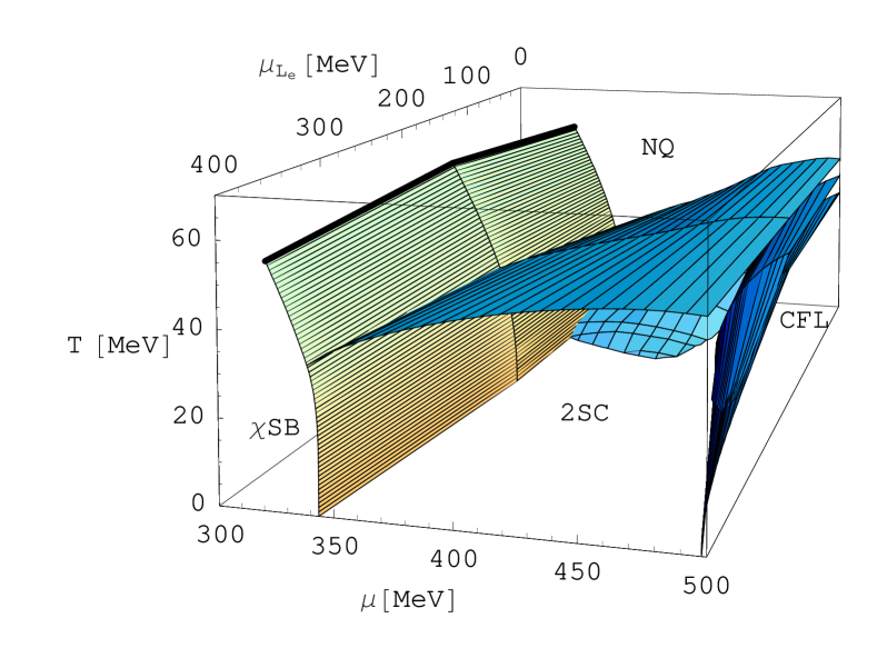
Figure 6: General structure of the phase diagram of neutral dense quark matter in the three-dimensional space spanned by the quark chemical potential $\mu$, the lepton-number chemical potential $\mu_{L_{e}}$, and the temperature $T$.

In order to discuss the structure of the phase diagram in more detail we proceed by showing several two-dimensional slices of it. These are obtained by keeping one of the chemical potentials, $\mu$ or $\mu_{L_{e}}$, fixed and varying the other two parameters.

3 $T$–$\mu$ phase diagram

We begin with presenting the phase diagrams at two fixed values of the lepton-number chemical potential, $\mu_{L_{e}}=200$ MeV (upper panel) and $\mu_{L_{e}}=400$ MeV (lower panel), in Fig. 7. The general effects of neutrino trapping can be understood by analyzing the similarities and differences between the diagrams with and without neutrino trapping.

Figure 7: The phase diagrams of neutral quark matter at fixed lepton-number chemical potentials $\mu_{L_{e}}=200$ MeV (upper panel), and $\mu_{L_{e}}=400$ MeV (lower panel), cf. Fig. 1 in the absence of neutrino trapping.

Here it is appropriate to note that a schematic version of the $T$–$\mu$ phase diagram at $\mu_{L_{e}}=200$ MeV was first presented in Ref. SRP, see the right panel of Fig. 4 there. If one ignores the complications due to the presence of the uSC phase and various gapless phases, the results of Ref. SRP are in qualitative agreement with the results presented here.

In order to understand the basic characteristics of different phases in the phase diagrams in Fig. 7, we also present the results for the dynamical quark masses, the gap parameters, and the charge chemical potentials. These are plotted as functions of the quark chemical potential in Figs. 8 and 9, for two different values of the temperature in the case of $\mu_{L_{e}}=200$ MeV and $\mu_{L_{e}}=400$ MeV, respectively.

Figure 8: Dependence of the quark masses, of the gap parameters, and of the electric and color charge chemical potentials on the quark chemical potential at a fixed temperature, $T=0~{}\mbox{MeV}$ (three upper panels) and $T=40~{}\mbox{MeV}$ (three lower panels). The lepton-number chemical potential is kept fixed at $\mu_{L_{e}}=200$ MeV.

Figure 9: Dependence of the quark masses, of the gap parameters, and of the electric and color charge chemical potentials on the quark chemical potential at a fixed temperature, $T=0~{}\mbox{MeV}$ (three upper panels), and $T=40~{}\mbox{MeV}$ (three lower panels). The lepton-number chemical potential is kept fixed at $\mu_{L_{e}}=400$ MeV.

As in the absence of neutrino trapping, see Fig. 1, there are roughly four distinct regimes in the phase diagrams in Fig. 7. At low temperature and low quark chemical potential, there is the $\chi$SB region. Here quarks have relatively large constituent masses which are close to the vacuum values, see Figs. 8 and 9. We note that the $\chi$SB phase is rather insensitive to the presence of a nonzero lepton-number chemical potential. With increasing $\mu_{L_{e}}$ the phase boundary is only slightly shifted to lower values of $\mu$. This is just another manifestation of the strengthening of the 2SC phase due to neutrino trapping.

With increasing temperature, the $\chi$SB phase turns into the normal quark matter phase, whose qualitative features are little affected by the lepton-number chemical potential.

The third regime is located at relatively low temperatures but at quark chemical potentials higher than in the $\chi$SB phase. In this region, the masses of the up and down quarks have already dropped to values well below their respective chemical potentials while the strange quark mass is still large, see left columns of panels in Figs. 8 and 9. As a consequence, up and down quarks are quite abundant but strange quarks are essentially absent.

It turns out that the detailed phase structure in this region is very sensitive to the lepton-number chemical potential. At $\mu_{L_{e}}=0$, the pairing between up and down quarks is strongly hampered by the constraints of neutrality and $\beta$ equilibrium, see Fig. 1. The situation changes dramatically with increasing the value of the lepton-number chemical potential, see Fig. 7. The low-temperature region of the normal phase of quark matter is replaced by the (g)2SC phase (e.g., at $\mu=400$ MeV, this happens at $\mu_{L_{e}}\simeq 110$ MeV). With $\mu_{L_{e}}$ increasing further, no qualitative changes happen in this part of the phase diagram, except that the area of the (g)2SC phase expands slightly.

Finally, the region in the phase diagram at low temperatures and large quark chemical potentials corresponds to phases in which the cross-flavor strange-nonstrange Cooper pairing becomes possible. In general, as the strength of pairing increases with the quark chemical potential, the system passes through regions of the gapless uSC (guSC), uSC, and gCFL phases and finally reaches the CFL phase. (Of course, the intermediate phases may not always be realized.) The effect of neutrino trapping, which grows with increasing the lepton-number chemical potential, is to push out the location of the strange-nonstrange pairing region to larger values of $\mu$. Of course, this is in agreement with the general arguments in Sec. 1.

As we mentioned earlier, the presence of the lepton-number chemical potential $\mu_{L_{e}}$ leads to a change of the quark Fermi momenta. This change in turn affects Cooper pairing of quarks, facilitating the appearance of some phases and suppressing others. As it turns out, there is also another qualitative effect due to a nonzero value of $\mu_{L_{e}}$. In particular, we find several new variants of gapless phases which did not exist at vanishing $\mu_{L_{e}}$. In Figs. 7 and 11, these are denoted by the same names, g2SC or gCFL, but with one or two primes added.

We define the g2SC^′ as the gapless two-flavor color-superconducting phase in which the gapless excitations correspond to $rd$–$gu$ and $gd$–$ru$ modes instead of the usual $ru$–$gd$ and $gu$–$rd$ ones, i.e., $u$ and $d$ flavors are exchanged as compared to the usual g2SC phase. The g2SC^′ phase becomes possible only when the value of $(\mu_{ru}-\mu_{gd})/2\equiv(\mu_{Q}+\mu_{3})/2$ is positive and larger than $\Delta_{3}$. The other phases are defined in a similar manner. In particular, the gCFL^′ phase, already introduced in Sec. 1, is indicated by the gapless $rs$–$bu$ mode, while the gCFL^′′ phase has both $gs$–$bd$ (as in the gCFL phase) and $rs$–$bu$ gapless modes. The definitions of all gapless phases are summarized in the following table:

Name	Gapless mode(s) $\epsilon(k)\sim|k-k_{F}^{\rm eff}|$	Diquark condensate(s)
g2SC	$ru$–$gd$, $gu$–$rd$	$\Delta_{3}$
g2SC′	$rd$–$gu$, $gd$–$ru$	$\Delta_{3}$
guSC	$rs$–$bu$	$\Delta_{2}$, $\Delta_{3}$
gCFL	$gs$–$bd$	$\Delta_{1}$, $\Delta_{2}$, $\Delta_{3}$
gCFL′	$rs$–$bu$	$\Delta_{1}$, $\Delta_{2}$, $\Delta_{3}$
gCFL′′	$gs$–$bd$, $rs$–$bu$	$\Delta_{1}$, $\Delta_{2}$, $\Delta_{3}$

4 Lepton fraction $Y_{L_{e}}$

Our numerical results for the lepton fraction $Y_{L_{e}}$ are shown in Fig. 10. The thick and thin lines correspond to two different fixed values of the lepton-number chemical potential, $\mu_{L_{e}}=200$ MeV and $\mu_{L_{e}}=400$ MeV, respectively. For a fixed value of $\mu_{L_{e}}$, we find that the lepton fraction changes only slightly with temperature. This is concluded from the comparison of the results at $T=0$ (solid lines), $T=20$ MeV (dashed lines), and $T=40$ MeV (dotted lines) in Fig. 10.

Figure 10: Dependence of the electron family lepton fraction $Y_{L_{e}}$ for $\mu_{L_{e}}=200$ MeV (thick lines) and $\mu_{L_{e}}=400$ MeV (thin lines) on the quark chemical potential at a fixed temperature, $T=0~{}\mbox{MeV}$ (solid lines), $T=20~{}\mbox{MeV}$ (dashed lines), and $T=40~{}\mbox{MeV}$ (dotted lines).

As is easy to check, at $T=40$ MeV, i.e., when Cooper pairing is not so strong, the $\mu$ dependence of $Y_{L_{e}}$ does not differ very much from the prediction in the simple two-flavor model in Sec. 1. By saying this, of course, one should not undermine the fact that the lepton fraction in Fig. 10 has a visible structure in the dependence on $\mu$ at $T=0$ and $T=20$ MeV. This indicates that quark Cooper pairing plays a nontrivial role in determining the value of $Y_{L_{e}}$.

Our numerical study shows that it is hard to achieve values of the lepton fraction more than about $0.05$ in the CFL phase. Gapless versions of the CFL phases, on the other hand, could accommodate a lepton fraction up to about $0.2$ or so, provided the quark and lepton-number chemical potentials are sufficiently large.

From Fig. 10, we can also see that the value of the lepton fraction $Y_{L_{e}}\approx 0.4$, i.e., the value expected at the center of the protoneutron star right after its creation, requires the lepton-number chemical potential $\mu_{L_{e}}$ in the range somewhere between $200$ MeV and $400$ MeV, or slightly higher. The larger the quark chemical potential $\mu$ the larger $\mu_{L_{e}}$ is needed. Then, in a realistic construction of a star, this is likely to result in a noticeable gradient of the lepton-number chemical potential at the initial time. This gradient may play an important role in the subsequent deleptonization due to neutrino diffusion through dense matter.

5 $T$–$\mu_{L_{e}}$ phase diagram

Now let us discuss the phase diagram in the plane of temperature and lepton-number chemical potential, keeping the quark chemical potential fixed. Two such slices of the phase diagram are presented in Fig. 11. The upper panel corresponds to a moderate value of the quark chemical potential, $\mu=400$ MeV. This could be loosely termed as the “outer core” phase diagram. The lower panel in Fig. 11 corresponds to $\mu=500$ MeV, and we could associate it with the “inner core” case. Note, however, that the terms “inner core” and “outer core” should not be interpreted literally here. The central densities of (proto-)neutron stars are subject to large theoretical uncertainties and, thus, are not known very well. In the model at hand, the case $\mu=400$ MeV (“outer core”) corresponds to a range of densities around $4\rho_{0}$, while the case $\mu=500$ MeV (“inner core”) corresponds to a range of densities around $10\rho_{0}$. These values are of the same order of magnitude that one typically obtains in models (see, e.g., Ref. prakash-et-al).

Figure 11: The phase diagrams of neutral quark matter in the plane of temperature and lepton-number chemical potential at two fixed values of quark chemical potential: $\mu=400$ MeV (upper panel) and $\mu=500$ MeV (lower panel). The triangle in the lower panel denotes the transition point from the CFL phase to the gCFL^′ phase at $T=0$.

At first sight, the two diagrams in Fig. 11 look so different that no obvious connection between them could be made. It is natural to ask, therefore, how such a dramatic change could happen with increasing the value of the quark chemical potential from $\mu=400$ MeV to $\mu=500$ MeV. In order to understand this, it is useful to place the corresponding slices of the phase diagram in the three-dimensional diagram in Fig. 6.

The $\mu=500$ MeV diagram corresponds to the right-hand-side surface of the bounding box in Fig. 6. This contains almost all complicated phases with strange-nonstrange cross-flavor pairing. The $\mu=400$ MeV diagram, on the other hand, is obtained by cutting the three-dimensional diagram with a plane parallel to the bounding surface, but going through the middle of the diagram. This part of the diagram is dominated by the 2SC and NQ phases. Keeping in mind the general structure of the three-dimensional phase diagram, it is also not difficult to understand how the two diagrams in Fig. 11 transform into each other.

Several comments are in order regarding the zero-temperature phase transition from the CFL to gCFL^′ phase, shown by a small black triangle in the phase diagram at $\mu=500$ MeV, see the lower panel in Fig. 11. The appearance of this transition is in agreement with the analytical result in Sec. 1. Moreover, the critical value of the lepton-number chemical potential also turns out to be very close to the estimate in Eq. (25). Indeed, by taking into account that $M_{s}\approx 214$ MeV and $\Delta_{2}\approx 76$ MeV, we obtain $\mu_{L_{e}}^{\rm(cr)}=\Delta_{2}-M_{s}^{2}/(2\mu)\approx 30$ MeV which agrees well with the numerical value.

Before concluding this subsection, we should mention that a schematic version of the phase diagram in $T$–$\mu_{L_{e}}$ plane was earlier presented in Ref. SRP, see the left panel in Fig. 4 there. In Ref. SRP, the value of the quark chemical potential was $\mu=460$ MeV, and therefore a direct comparison is not straightforward. One can see, however, that the diagram of Ref. SRP fits naturally into the three-dimensional diagram in Fig. 6. Also, the diagram of Ref. SRP is topologically close to the $\mu=500$ MeV phase diagram shown in the lower panel of Fig. 11. The quantitative difference is not surprising: the region of the (g)CFL phase is considerably larger at $\mu=500$ MeV than at $\mu=460$ MeV.

5 Conclusions

Here we discussed the phase diagram of neutral three-flavor quark matter in the space of three parameters: temperature $T$, quark chemical potential $\mu$, and lepton-number chemical potential $\mu_{L_{e}}$. The analysis is performed in the mean-field approximation in the phenomenologically motivated NJL model introduced in Ref. RKH. Constituent quark masses are treated as dynamically generated quantities. The overall structure of the three-dimensional phase diagram is summarized in Fig. 6 and further detailed in several two-dimensional slices, see Figs. 1, 7 and 11.

By making use of simple model-independent arguments, as well as detailed numerical calculations in the framework of an NJL-type model, we find that neutrino trapping helps Cooper pairing in the 2SC phase and suppresses the CFL phase. In essence, this is the consequence of satisfying the electric neutrality constraint in the quark system. In two-flavor quark matter, the (positive) lepton-number chemical potential $\mu_{L_{e}}$ helps to provide extra electrons without inducing a large mismatch between the Fermi momenta of up and down quarks. With reducing the mismatch, of course, Cooper pairing gets stronger. This is in sharp contrast to the situation in the CFL phase of quark matter, which is neutral in the absence of electrons. Additional electrons due to large $\mu_{L_{e}}$ can only put extra stress on the system.

In application to protoneutron stars, the findings presented here suggest that the CFL phase is very unlikely to appear during the early stage of the stellar evolution before the deleptonization is completed. If color superconductivity occurs there, the 2SC phase is the best candidate for the ground state. In view of this, it might be quite natural to suggest that matter inside protoneutron stars contains little or no strangeness (just as the cores of the progenitor stars) during the early times of their evolution. In this connection, it is appropriate to recall that neutrino trapping also suppresses the appearance of strangeness in the form of hyperonic matter and kaon condensation.[29] The situation in quark matter, therefore, is a special case of a generic property.

After the deleptonization occurs, it is possible that the ground state of matter at high density in the central region of the star is the CFL phase. This phase contains a large number of strange quarks. Therefore, an abundant production of strangeness should happen right after the deleptonization in the protoneutron star. If realized in nature, in principle this scenario may have observational signatures.

Acknowledgments

This review is based on work of Refs. pd-mass and pd-nu. This work was supported in part by the Virtual Institute of the Helmholtz Association under grant No. VH-VI-041, by the Gesellschaft für Schwerionenforschung (GSI), and by the Deutsche Forschungsgemeinschaft (DFG).

References

- [1] K. Rajagopal and F. Wilczek, hep-ph/0011333; M. Alford, Ann. Rev. Nucl. Part. Sci. 51, 131 (2001); T. Schäfer, hep-ph/0304281; D. H. Rischke, Prog. Part. Nucl. Phys. 52, 197 (2004); M. Buballa, Phys. Rep. 407, 205 (2005); H.-C. Ren, hep-ph/0404074; M. Huang, Int. J. Mod. Phys. E 14, 675 (2005); I. A. Shovkovy, Found. Phys. 35, 1309 (2005).
- [2] M. Alford and K. Rajagopal, JHEP 0206, 031 (2002).
- [3] A. W. Steiner, S. Reddy, and M. Prakash, Phys. Rev. D 66, 094007 (2002).
- [4] M. Huang, P. F. Zhuang, and W. Q. Chao, Phys. Rev. D 67, 065015 (2003).
- [5] I. Shovkovy and M. Huang, Phys. Lett. B 564, 205 (2003); M. Huang and I. Shovkovy, Nucl. Phys. A 729, 835 (2003).
- [6] M. Alford, C. Kouvaris, and K. Rajagopal, Phys. Rev. Lett. 92, 222001 (2004); Phys. Rev. D 71, 054009 (2005).
- [7] S. B. Rüster, I. A. Shovkovy, and D. H. Rischke, Nucl. Phys. A 743, 127 (2004).
- [8] M. G. Alford, K. Rajagopal, and F. Wilczek, Nucl. Phys. B537, 443 (1999).
- [9] I. A. Shovkovy and L. C. R. Wijewardhana, Phys. Lett. B 470, 189 (1999); T. Schäfer, Nucl. Phys. B575, 269 (2000).
- [10] K. Iida, T. Matsuura, M. Tachibana, and T. Hatsuda, Phys. Rev. Lett. 93, 132001 (2004).
- [11] M. Alford, K. Rajagopal, and F. Wilczek, Phys. Lett. B 422, 247 (1998); R. Rapp, T. Schäfer, E. V. Shuryak, and M. Velkovsky, Phys. Rev. Lett. 81, 53 (1998).
- [12] D. T. Son, Phys. Rev. D 59, 094019 (1999); T. Schäfer and F. Wilczek, Phys. Rev. D 60, 114033 (1999); D. K. Hong, V. A. Miransky, I. A. Shovkovy, and L. C. R. Wijewardhana, Phys. Rev. D 61, 056001 (2000); R. D. Pisarski and D. H. Rischke, Phys. Rev. D 61, 051501(R) (2000); W. E. Brown, J. T. Liu, and H.-C. Ren, Phys. Rev. D 61, 114012 (2000).
- [13] K. Fukushima, C. Kouvaris, and K. Rajagopal, Phys. Rev. D 71, 034002 (2005).
- [14] I. A. Shovkovy, S. B. Rüster, and D. H. Rischke, J. Phys. G 31, S849 (2005).
- [15] S. B. Rüster, V. Werth, M. Buballa, I. A. Shovkovy, and D. H. Rischke, Phys. Rev. D 72, 034004 (2005).
- [16] S. B. Rüster, V. Werth, M. Buballa, I. A. Shovkovy, and D. H. Rischke, hep-ph/0509073.
- [17] H. Abuki, M. Kitazawa, and T. Kunihiro, Phys. Lett. B 615, 102 (2005).
- [18] D. Blaschke, S. Fredriksson, H. Grigorian, A. M. Öztaş, and F. Sandin, Phys. Rev. D 72, 065020 (2005).
- [19] H. Abuki and T. Kunihiro, hep-ph/0509172.
- [20] F. Neumann, M. Buballa, and M. Oertel, Nucl. Phys. A 714, 481 (2003); I. Shovkovy, M. Hanauske, and M. Huang, Phys. Rev. D 67, 103004 (2003); S. Reddy and G. Rupak, Phys. Rev. C 71, 025201 (2005).
- [21] M. G. Alford, J. A. Bowers, and K. Rajagopal, Phys. Rev. D 63, 074016 (2001); R. Casalbuoni, R. Gatto, M. Mannarelli, and G. Nardulli, Phys. Rev. D 66, 014006 (2002); I. Giannakis, J. T. Liu, and H.-C. Ren, Phys. Rev. D 66, 031501(R) (2002).
- [22] K. Rajagopal and F. Wilczek, Phys. Rev. Lett. 86, 3492 (2001).
- [23] M. Huang and I. A. Shovkovy, Phys. Rev. D 70, 051501(R) (2004); Phys. Rev. D 70, 094030 (2004); R. Casalbuoni, R. Gatto, M. Mannarelli, G. Nardulli, and M. Ruggieri, Phys. Lett. B 605, 362 (2005); I. Giannakis and H.-C. Ren, Phys. Lett. B 611, 137 (2005); M. Alford and Q. H. Wang, J. Phys. G 31, 719 (2005).
- [24] K. Fukushima, hep-ph/0512138.
- [25] T. Schäfer, Phys. Rev. D 62, 094007 (2000); M. Buballa, J. Hošek, and M. Oertel, Phys. Rev. Lett. 90, 182002 (2003); A. Schmitt, Q. Wang, and D. H. Rischke, Phys. Rev. D 66, 114010 (2002); Phys. Rev. Lett. 91, 242301 (2003); A. Schmitt, Phys. Rev. D 71, 054016 (2005); D. N. Aguilera, D. Blaschke, M. Buballa, and V. L. Yudichev, Phys. Rev. D 72, 034008 (2005).
- [26] P. F. Bedaque and T. Schäfer, Nucl. Phys. A 697, 802 (2002); D. B. Kaplan and S. Reddy, Phys. Rev. D 65, 054042 (2002); A. Kryjevski, D. B. Kaplan, and T. Schäfer, Phys. Rev. D 71, 034004 (2005); A. Kryjevski, hep-ph/0508180; T. Schäfer, hep-ph/0508190.
- [27] M. Huang, hep-ph/0504235; D. K. Hong, hep-ph/0506097.
- [28] E. V. Gorbar, M. Hashimoto, and V. A. Miransky, Phys. Lett. B 632, 305 (2006).
- [29] M. Prakash, I. Bombaci, M. Prakash, P. J. Ellis, J. M. Lattimer, and R. Knorren, Phys. Rept. 280, 1 (1997).
- [30] M. Buballa, Phys. Lett. B 609, 57 (2005); M. M. Forbes, Phys. Rev. D 72, 094032 (2005).
- [31] P. Rehberg, S. P. Klevansky, and J. Hüfner, Phys. Rev. C 53, 410 (1996).
- [32] M. Buballa and I. A. Shovkovy, Phys. Rev. D 72, 097501 (2005).
- [33] A. W. Steiner, Phys. Rev. D 72, 054024 (2005).
- [34] J. I. Kapusta, Finite-temperature field theory, (University Press, Cambridge, 1989).
- [35] M. Asakawa and K. Yazaki, Nucl. Phys. A 504, 668 (1989); Nucl. Phys. B 538, 215 (1999); O. Scavenius, A. Mocsy, I. N. Mishustin, and D. H. Rischke, Phys. Rev. C 64, 045202 (2001).
- [36] M. Buballa and M. Oertel, Nucl. Phys. A 703, 770 (2002).
- [37] Z. Fodor and S. D. Katz, JHEP 0404, 050 (2004).