First application of the continuum-QRPA to description of the double beta decay

Abstract

A continuum-QRPA approach to calculation of the $2\nu\beta\beta$- and $0\nu\beta\beta$-amplitudes has been formulated. For ¹³⁰Te a regular suppression (about 20%) of the high-multipole contributions to the $0\nu\beta\beta$-amplitude has been found which can be associated with additional ground state correlations appearing from the transitions to collective states in the continuum. At the same time the total calculated $0\nu\beta\beta$-amplitude for ¹³⁰Te gets suppressed by about 20% as compared to the result of the usual, discretized, QRPA.

1 Introduction

At present, the most elaborated analysis of the uncertainties in the $0\nu\beta\beta$-decay nuclear matrix elements $M^{0\nu}$ calculated within the QRPA and RQRPA has been performed in the recent works [1, 2]. The experimental $2\nu\beta^{-}\beta^{-}$-decay rate has been used to adjust the most relevant parameter, the strength $g_{pp}$ of the particle-particle interaction. With such a procedure the values of $M^{0\nu}$ have been shown to become essentially independent on the size of the single-particle (s.p.) basis. Furthermore, the $M^{0\nu}$’s have been demonstrated to be also rather stable with respect to the possible quenching of the axial vector strength $g_{A}$, as well as to the uncertainties of parameters describing the short range nucleon correlations.

The calculations in [1, 2] have been performed within “the standard QRPA” scheme in which the BCS ground state and the spectrum of the excited states are built on a discrete s.p. basis. However, in order to really assess the uncertainty of the QRPA calculations of the $M^{0\nu}$ one has to address the questions regarding the accuracy of “the standard QRPA” itself, and whether there are not some important contributions missing.

The accepted procedure [1, 2] of averaging the results of the calculations performed with different choices of the model space size looks rather weakly justified. One can expect a priori that enlargement of the model space should lead to more accurate results (in other words, any basis truncation leads to an uncertainty). The usual statement that “in the QRPA one can include essentially an unlimited set of single-particle states” [1] can be considered at presence only as principally correct, but not realized in practice. In reality, the large number of the major shells $N\gg 1$ in the QRPA calculations can only be achieved by adding low-lying major shells composed of the bound states. Basically, only one major shell lying higher than the Fermi-shell one can be considered, because one immediately encounters principal limitations of the approximation of the single-particle continuum by discrete levels. Neglecting the single-particle continuum leads to a missing strength in the usual QRPA calculations, especially for description of the high-multipole excitations with $L\geq 2$ .

The contribution of these multipoles to $M^{0\nu}$ is particularly important because the monopole (Fermi + Gamow-Teller) one is suppressed due to the symmetry constrains (see, e.g., the multipole decomposition of $M^{0\nu}$ in Fig. 5 of [2]; for a recent discussion how the SU(4)-symmetry violation by the particle-particle interaction affects $M^{2\nu}$ see [3]). Furthermore, the pure pairing contribution to $M^{0\nu}$ is almost completely (by an order of magnitude) suppressed by the ground state correlations, short-range correlations etc., therefore fine effects can be expected to play an important role.

The question about the dependence of the QRPA results on the s.p.-basis size as a source of the uncertainties in the calculated $M^{0\nu}$’s would be completely resolved if one could include the entire s.p. basis into the calculation scheme. The only possible way principally to perform such ultimate-basis QRPA calculations is provided within the continuum-QRPA. Also, to have an alternative formulation of the QRPA can help to promote our understanding of the current QRPA results and their deficiencies to a higher level. In particular, the continuum-QRPA provides a regular way of using realistic wave functions of the continuum states in terms of the Green’s functions and there is no need to approximate them by the oscillator ones.

Two principal effects of the inclusion of the s.p. continuum within the pn-QRPA, which affect $M^{0\nu}$’s in an opposite way, can be expected. First, pairing in the continuum can increase respective $0\nu\beta\beta$ sum rules (the smallness of the $\Delta/E$ in the continuum can be compensated by a large corresponding partial s.p. matrix element). Second, additional g.s. correlations can appear due to collective multipole states in the continuum that decreases $M^{0\nu}$. It is noteworthy that at the moment the continuum-QRPA consistently including pairing in the continuum has not been formulated yet and only the continuum-QRPA with the pairing realized on a discrete basis can be used.

The principal aim of this work is to formulate for the first time a method to calculate the double beta decay matrix elements within the continuum-QRPA.

2 Continuum-QRPA

The continuum-RPA has been used for a long time to successfully describe structure and decay properties of various giant resonances and their high-lying overtones embedded in the single-particle continuum. However, to apply the continuum-RPA in open-shell nuclei one has to take the nucleon pairing into consideration and develop a continuum-QRPA approach. The approach should account for the important effects of particle-particle interaction along with the usual particle-hole one. Such a continuum-QRPA approach has been developed in [4, 5]. In [4] the approach has been applied to the analysis of the low-energy part of the Gamow-Teller (GT) strength distribution for description of the single-beta decay relevant to astrophysical applications.

2.1 QRPA equations in the coordinate representation

The system of homogeneous equations for the forward and backward amplitudes $X^{(J^{\pi}s)}_{\pi\nu}$ and $Y^{(J^{\pi}s)}_{\pi\nu}$, respectively, is usually solved to calculate the energies $\omega_{s}$ and the wave functions $|J\mu,s\rangle$ of the isobaric nucleus within the pn-QRPA (see, e.g., [6]). It is impossible to handle the infinite number of the amplitudes $X,Y$ if one wants to include the single-particle continuum. Instead, by going into the coordinate representation the pn-QRPA can be reformulated in equivalent terms of four-component radial transition density $\{\varrho^{(J^{\pi}s)}_{I}\}\ (I=1,\dots 4)$. The components are determined by the standard QRPA amplitudes $X$ and $Y$ as follows:

$$\varrho^{(J^{\pi}s)}_{I}(r)=\sum\limits_{\pi\nu}R^{(J^{\pi}s)\pi\nu}_{I}\,\chi_{\pi\nu}(r),$$ (1)

$$\left({\begin{array}[]{c}R^{\pi\nu}_{p-h}\\ R^{\pi\nu}_{h-p}\\ R^{\pi\nu}_{p-p}\\ R^{\pi\nu}_{h-h}\end{array}}\right)=\left({\begin{array}[]{c}u_{\pi}v_{\nu}X_{\pi\nu}+v_{\pi}u_{\nu}Y_{\pi\nu}\\ u_{\pi}v_{\nu}Y_{\pi\nu}+v_{\pi}u_{\nu}X_{\pi\nu}\\ u_{\pi}u_{\nu}X_{\pi\nu}-v_{\pi}v_{\nu}Y_{\pi\nu}\\ u_{\pi}u_{\nu}Y_{\pi\nu}-v_{\pi}v_{\nu}X_{\pi\nu}\end{array}}\right)$$ (10)

where $u,~{}v$ are the coefficients of Bogolyubov transformation, $\chi_{\pi\nu}(r)=t^{(J)}_{(\pi)(\nu)}\,\chi_{\pi}(r)\chi_{\nu}(r)$ with $t^{(J)}_{(\pi)(\nu)}=\frac{1}{\sqrt{2J+1}}\langle\pi\|T_{JLS}\|\nu\rangle$ being the reduced matrix element of the spin-angular tensor $T_{JLS\mu}$ and $\chi_{\pi}(r)$ ($\chi_{\nu}(r)$) being the radial wave function of a single-particle proton (neutron) state. Hereafter we shall systematically omit the superscript “${J^{\pi}s}$” when it does not lead to a confusion.

According to the definition (1), the elements $\varrho_{1},\varrho_{2},\varrho_{3},\varrho_{4}$ can be called the particle-hole, hole-particle, hole-hole and particle-particle components of the transition density, respectively. In particular, the transition matrix element to the state $|s,J\mu\rangle$ corresponding to a probing particle-hole operator $\hat{V}^{(-)}_{J\mu}=\sum_{a}V_{J}(r_{a})T_{JLS\mu}\ \tau^{-}_{a}$ is determined by the element $\varrho_{1}$:  $\int\varrho^{(J^{\pi},s)}_{1}(r)V_{J}(r)\,dr$.

The pn-QRPA system of equations for the elements $\varrho_{i}^{(J^{\pi}s)}$ is as follows:

$$\varrho^{(J^{\pi}s)}_{I}(r)=\sum\limits_{K}\int A^{(J^{\pi})}_{IK}(rr^{\prime},\omega=\omega_{s})\,F^{(J^{\pi})}_{K}(r^{\prime}r^{\prime\prime})\,\varrho^{(J^{\pi}s)}_{K}(r^{\prime\prime})\,dr^{\prime}dr^{\prime\prime},$$ (11)

or schematically, denoting all the integrations and summations as $\{\dots\}$, $\varrho=\{AF\varrho\}$, where $F^{(J^{\pi})}_{K}(r_{1}r_{2})$ represents the residual interaction in $K$-channel ($K=1,2$ — p-h channel, $K=3,4$ — p-p channel) after separation of the spin-angular variables. The $4\times 4$ matrix $A_{IK}(r_{1}r_{2},\omega)$ is the radial part of the free two-quasiparticle propagator. The expressions for the elements of the free two-quasiparticle propagator $A_{IK}$ can be obtained by making use of the regular and anomalous single-particle Green’s functions for Fermi-systems with nucleon pairing in an analogous way to how it was done in the monograph [7] to describe the Fermi-system response to a single-particle probing operator acting in the neutral channel [5]. The corresponding analytical representations for the elements $A_{IK}(r_{1}r_{2},\omega)$are:

$$A_{IK}(r_{1}r_{2},\omega)=\sum\limits_{\pi\nu}\,\chi_{\pi\nu}(r_{1})\chi_{\pi\nu}(r_{2})\,A^{\pi\nu}_{IK}(\omega);\ \ \ \ A^{\pi\nu}_{IK}=A^{\pi\nu}_{KI}$$ (12)

$$A^{\pi\nu}_{11}=\displaystyle\frac{u^{2}_{\pi}v^{2}_{\nu}}{\omega-E_{\pi}-E_{\nu}}+\frac{u^{2}_{\nu}v^{2}_{\pi}}{-\omega-E_{\pi}-E_{\nu}},\ \ A^{\pi\nu}_{33}=\frac{u^{2}_{\pi}u^{2}_{\nu}}{\omega-E_{\pi}-E_{\nu}}+\frac{v^{2}_{\nu}v^{2}_{\pi}}{-\omega-E_{\pi}-E_{\nu}},$$

$$A^{\pi\nu}_{12}=A^{\pi\nu}_{34}=\displaystyle\frac{u_{\pi}v_{\pi}v_{\nu}u_{\nu}}{\omega-E_{\pi}-E_{\nu}}+\frac{u_{\pi}v_{\pi}v_{\nu}u_{\nu}}{-\omega-E_{\pi}-E_{\nu}}$$

$$A^{\pi\nu}_{13}=u_{\nu}v_{\nu}\displaystyle(\frac{u^{2}_{\pi}}{\omega-E_{\pi}-E_{\nu}}-\frac{v^{2}_{\pi}}{-\omega-E_{\pi}-E_{\nu}}),\ \ A^{\pi\nu}_{14}=u_{\pi}v_{\pi}(\frac{v^{2}_{\nu}}{\omega-E_{\pi}-E_{\nu}}-\frac{u^{2}_{\nu}}{-\omega-E_{\pi}-E_{\nu}})\ ,$$

$$A^{\pi\nu}_{22}(\omega)=A^{\pi\nu}_{11}(-\omega),\ \ A^{\pi\nu}_{44}(\omega)=A^{\pi\nu}_{33}(-\omega),\ \ A^{\pi\nu}_{23}(\omega)=A^{\pi\nu}_{14}(-\omega),\ \ A^{\pi\nu}_{24}(\omega)=A^{\pi\nu}_{13}(-\omega).$$

The total two-quasiparticle propagator $\tilde{A}$ that includes the QRPA iterations of the p-h and p-p interactions satisfies a Bethe-Goldstone-type integral equation:

$$\tilde{A}=A+\{AF\tilde{A}\}$$

and has the following spectral decomposition:

$$\displaystyle\tilde{A}^{(J^{\pi})}_{IK}(r_{1}r_{2},\omega)=\sum_{s}\frac{\varrho^{(J^{\pi}s)}_{I}(r_{1})\varrho^{(J^{\pi}s)}_{K}(r_{2})}{\omega-\omega_{s}+i\delta}-\sum_{s}\frac{\varrho^{(J^{\pi}s)}_{I}(r_{1})\varrho^{(J^{\pi}s)}_{K}(r_{2})}{\omega+\omega_{s}-i\delta}$$ (13)

Thus, all the necessary information about the QRPA solutions resides in the poles of $\tilde{A}^{(J^{\pi})}$.

2.2 Strength functions

One can use $\mathop{\rm Im}\nolimits\tilde{A}$ to calculate different strength functions. Strength function corresponding to a charge-exchange single-particle probing operator

$$\hat{V}^{(\mp)}_{J\mu}=\sum_{a}V_{J}(r_{a})T_{JLS\mu}(n_{a})\tau_{a}^{(\mp)}$$ (14)

acting in $\beta^{(\mp)}$-cnannel is defined by the usual expression:

$$S^{(\mp)}(\omega)=\sum\limits_{s}\left|\langle s|\hat{V}^{(\mp)}_{J\mu}|0\rangle\right|^{2}\delta(\omega-\omega_{s}^{\mp})$$

with $\omega_{s}^{\mp}=E_{s}^{\mp}-E_{0}$ being the excitation energy of the corresponding isobaric nucleus measured from the ground state of the parent nucleus. Making use of the spectral decomposition (13) one can easily verify the following integral representations of the strength functions in term of $\mathop{\rm Im}\nolimits\tilde{A}$:

$$S^{(-)}(\omega^{-})=-\frac{1}{\pi}\mathop{\rm Im}\nolimits\int V_{J}(r_{1})\tilde{A}_{11}^{(J^{\pi})}(r_{1}r_{2};\omega)V_{J}(r_{2})\,dr_{1}dr_{2}$$ (15)

$$S^{(+)}(\omega^{+})=-\frac{1}{\pi}\mathop{\rm Im}\nolimits\int V_{J}(r_{1})\tilde{A}_{22}^{(J^{\pi})}(r_{1}r_{2};\omega)V_{J}(r_{2})\,dr_{1}dr_{2}$$ (16)

or, schematically,

$$S^{(-)}_{V}(\omega^{-})=-\frac{1}{\pi}\left\{V\tilde{A}_{11}(\omega)V\right\}\ \ \ \ S^{(+)}_{V}(\omega^{+})=-\frac{1}{\pi}\left\{V\tilde{A}_{22}(\omega)V\right\}$$

with $\omega^{\mp}=\omega\pm(\lambda_{p}-\lambda_{n})$. The calculated pn-QRPA spectrum in $\omega$ is to be shifted in energy in order to be measured from the ground state of the parent nucleus. It has to do with the fact that in the QRPA the BCS hamiltonian $\hat{H}-\lambda_{p}\hat{Z}-\lambda_{n}\hat{N}$ is used.

One can also define a non-diagonal strength function like

$$S^{(--)}_{V}(\omega)=\sum\limits_{s}\langle 0^{\prime}|\hat{V}^{(-)}_{J\bar{\mu}}|s\rangle\langle s|\hat{V}^{(-)}_{J\mu}|0\rangle\delta(\omega-\omega^{\prime}_{s})$$ (17)

with $\omega^{\prime}_{s}=E_{s}-(E_{0}+E_{0^{\prime}})/2$. Such a strength function is closely related to the amplitude of the $2\nu\beta\beta$-decay. To calculate $S^{(--)}_{V}(\omega)$ within the pn-QRPA one faces the usual problem that the spectrum $|s\rangle$ comes out slightly different when calculated starting from the initial or final ground states. Identifying the BCS vacuum $|0^{\prime}\rangle$ with that of $|0\rangle$ one gets

$$S^{(--)}(\omega^{-})=-\frac{1}{\pi}\mathop{\rm Im}\nolimits\int V_{J}(r_{1})\tilde{A}_{12}^{(J^{\pi})}(r_{1}r_{2};\omega)V_{J}(r_{2})\,dr_{1}dr_{2}$$ (18)

or, alternatively, identifying $|0\rangle$ with $|0^{\prime}\rangle$

$$S^{(--)}(\omega^{+})=-\frac{1}{\pi}\mathop{\rm Im}\nolimits\int V_{J}(r_{1})\tilde{A^{\prime}}^{(J^{\pi})}_{12}(r_{1}r_{2};\omega)V_{J}(r_{2})\,dr_{1}dr_{2}$$ (19)

where $\tilde{A}^{\prime}$ is calculated with respect to $|0^{\prime}\rangle$.

To calculate the strength functions, it is more convenient to use a system of inhomogeneous cQRPA equations in $\beta^{-}$-channel:

$$S^{(-)}_{V}(\omega^{-})=-\frac{1}{\pi}\mathop{\rm Im}\nolimits\sum\limits_{K}\int V(r_{1})\,A_{1K}(r_{1}r_{2},\omega)\,\tilde{V}_{K}(r_{2},\omega)\,dr_{1}dr_{2},$$ (20)

$$S^{(--)}_{V}(\omega^{-})=-\frac{1}{\pi}\mathop{\rm Im}\nolimits\sum\limits_{K}\int V(r_{1})\,A_{2K}(r_{1}r_{2},\omega)\,\tilde{V}_{K}(r_{2},\omega)\,dr_{1}dr_{2},$$ (21)

$$\tilde{V}_{I}(r,\omega)=V(r)\delta_{I1}+\sum\limits_{K}\int F_{K}(rr_{1})\,A_{IK}(r_{1}r_{2},\omega)\,\tilde{V}_{K}(r_{2},\omega)\,dr_{1}dr_{2},$$ (22)

or, in $\beta^{+}$-channel:

$$S^{(+)}_{V}(\omega^{+})=-\frac{1}{\pi}\mathop{\rm Im}\nolimits\sum\limits_{K}\int V(r)\,A_{2K}(r_{1}r_{2},\omega)\,\tilde{V}_{K}(r_{2},\omega)\,dr_{1}dr_{2},$$ (23)

$$\tilde{V}_{I}(r,\omega)=V(r)\delta_{I2}+\sum\limits_{K}\int F_{K}(rr_{1})\,A_{IK}(r_{1}r_{2},\omega)\,\tilde{V}_{K}(r_{2},\omega)\,dr_{1}dr_{2}.$$ (24)

2.3 Taking the s.p. continuum into consideration

Up to now the way of taking the s.p. continuum into consideration has not been specified explicitly within this formulation of the pn-QRPA. If one lets the double sums in (12) run just over the bound proton and neutron s.p. states, the version of the pn-QRPA presented in two preceeding sections is fully equivalent to the usual discretized one formulated in terms of $X$ and $Y$ amplitudes. We make use of this fact and compare discrete-QRPA results calculated in these two different, but formally equivalent, ways in order to check the consistency of the scheme.

To take the s.p. continuum into consideration, one has to do the following in (12):

1. To approximate $v_{i},\ u_{i}$ and $E_{i}$ by their no-pairing values $v=0(1),\ u=1(0)$, $E=|\varepsilon-\lambda|$ for those s.p. states which lie far from the chemical potential (i.e. $|\varepsilon-\lambda|\gg\Delta$). The accuracy of this approximation is $\frac{\Delta}{|\varepsilon-\lambda|}$.

2. To use the s.p. Green function: $g_{(\alpha)}(r_{1}r_{2},\varepsilon)=\displaystyle\sum_{\alpha}\frac{\chi_{\alpha}(r_{1})\chi_{\alpha}(r_{2})}{\varepsilon-\varepsilon_{\alpha}}$ to explicitly perform the sum over the s.p. states in the continuum.

As an example of such an approach we present here the final expression for $A_{11}$:

$$A_{11}(r_{1}r_{2},\omega) = \sum\limits_{\nu}\mathop{{\sum}^{\prime}}\limits_{\pi}\frac{v^{2}_{\nu}u^{2}_{\pi}\chi_{\pi\nu}(r_{1})\chi_{\pi\nu}(r_{2})}{\omega-E_{\pi}-E_{\nu}}+\mathop{{\sum}^{\prime}}\limits_{\nu}\sum\limits_{\pi<\pi_{min}}\frac{v^{2}_{\nu}\chi_{\pi\nu}(r_{1})\chi_{\pi\nu}(r_{2})}{\omega-E_{\nu}+\lambda_{\pi}-\varepsilon_{\pi}}$$ (25)

$$+\sum\limits_{\nu(\pi)}\left(t^{(J)}_{(\pi)(\nu)}\right)^{2}\chi_{\nu}(r_{1})\chi_{\nu}(r_{2})~{}v^{2}_{\nu}g^{\prime}_{(\pi)}(r_{1}r_{2},\lambda_{\pi}+\omega-E_{\nu})$$

$$+\left\{\pi\leftrightarrow\nu,\omega\to-\omega\right\}$$

where the projected s.p. Green’s function is $g^{\prime}_{(\pi)}(r_{1}r_{2},\varepsilon)=g_{(\pi)}(r_{1}r_{2},\varepsilon)-\displaystyle\mathop{{\sum}^{\prime}}\limits_{\pi}\frac{\chi_{\pi}(r_{1})\chi_{\pi}(r_{2})}{\varepsilon-\varepsilon_{\pi}}$. The primed sum $\mathop{{\sum}^{\prime}}$ runs over only those s.p. states which comprise the BCS basis (for instance, all proton s.p. states $\pi_{min}\leq\pi\leq\pi_{max}$).

This continuum-QRPA method has been applied in our recent paper [5] to describe the Fermi and Gamow-Teller strength distributions in semi-magic nuclei.

2.4 Description of the $\beta\beta$-decay within the cQRPA

The spectral decomposition of $\tilde{A}$ (13) can be used for calculation of $\beta\beta$-decay matrix elements in a way similar to the one described in Sec. 2.2. For instance, the $2\nu\beta\beta$-amplitude can be calculated according to the following expression:

$$M^{2\nu}_{GT}=-\frac{3}{2}\int\tilde{A}^{(1)}_{12}(r_{1}r_{2};\omega=0)\,dr_{1}dr_{2}\ \ +\ \ \delta M^{2\nu}_{GT}$$ (26)

$$\delta M^{2\nu}_{GT}=\frac{3\delta E}{\pi}\int d\omega\frac{\int\mathop{\rm Im}\nolimits\tilde{A}_{12}^{(1)}(r_{1}r_{2};\omega)\,dr_{1}dr_{2}}{(\omega+\delta E)\omega}$$

where $\delta E=Q_{\beta\beta}/2+m_{e}c^{2}+\lambda_{p}-\lambda_{n}$. We use in deriving (26) the approximation that the BCS vacuum $|0^{\prime}\rangle$ of the final g.s. is taken to be the same as $|0\rangle$ of the initial g.s. The expression (26) can be further rewritten in terms of the effective field $\tilde{V}_{K}$ (22):

$$M^{2\nu}_{GT}=-\frac{3}{2}\sum_{K}\int A^{(1)}_{2K}(r_{1}r_{2};\omega=0)\tilde{V}_{K}(r_{2};\omega=0)\,dr_{1}dr_{2}\ \ +\ \ \delta M^{2\nu}_{GT}$$ (27)

$$\delta M^{2\nu}_{GT}=\frac{3\delta E}{\pi}\int d\omega\frac{\sum_{K}\int\mathop{\rm Im}\nolimits A_{2K}^{(1)}(r_{1}r_{2};\omega)\tilde{V}_{K}(r_{2};\omega)\,dr_{1}dr_{2}}{(\omega+\delta E)\omega}$$

The same procedure can be applied to calculate within the cQRPA the matrix element of a two-body operator

$$\hat{V}^{(--)}_{2}=\sum_{ab}\sum_{JLS\mu}V_{JL}(r_{a},r_{b})T_{JLS\mu}(n_{a})T^{*}_{JLS\mu}(n_{b})\tau_{a}^{(-)}\tau_{b}^{(-)}$$ (28)

between the ground states $|0\rangle$ and $|0^{\prime}\rangle$ as a sum of all partial contributions $M^{(JL)}$:

$$M^{(--)}=\langle 0^{\prime}|\hat{V}^{(--)}_{2}|0\rangle=\displaystyle\sum_{JL}M^{(JL)}$$ (29)

$$M^{(JL)}=-\frac{(2J+1)}{\pi}\int d\omega\ \int V_{JL}(r_{1},r_{2})\mathop{\rm Im}\nolimits\tilde{A}^{(J^{\pi})}_{12}(r_{1}r_{2};\omega)\,dr_{1}dr_{2}$$

(the identification of the ground states described above has to be done).

The neutrino potential $\hat{V}^{(--)}_{2}$ in the simpliest (but rather rough) Coulomb approximation has the well-known partial radial components $V_{JL}(r_{1},r_{2})=\frac{4\pi}{2L+1}\frac{1}{r_{>}}\left(\frac{r_{<}}{r_{>}}\right)^{L}$ ($r_{<}=min(r_{1},r_{2}),\ r_{>}=max(r_{1},r_{2})$). When the Jastrow factor (to account for the short range correlations) and the energy dependence of the neutrino propagator are considered, the decomposition of the neutrino potential over the Legandre polinomials (28) can be done numerically.

3 First calculation results

For the first calculations of $M^{2\nu}$ and $M^{0\nu}$ within the continuum-QRPA we adopt a rather simple nuclear Hamiltonian similar to that used in [8, 9]. The chosen nuclear mean field $U(x)$ consists of the phenomenological isoscalar part $U_{0}(x)$ along with the isovector $U_{1}(x)$ and the Coulomb $U_{C}(x)$ parts, both calculated consistently in the Hartree approximation (see [5]). The residual particle-hole interaction as well as the particle-particle interaction in both the neutral (pairing) and charge-exchange channels are chosen in the form of the zero-range, $\delta$-functional, forces (hereafter all the strength parameters of the residual interactions are given in units of 300 MeV$\cdot$ fm³).

Table 1: The fitted parameters $f^{1}_{ph}$, $g^{1}_{pp}$ and the calculated $M^{0\nu}$ for ¹³⁰Te ($g_{A}=1.25$).

QRPA	$f^{1}_{ph}$	$g^{1}_{pp}$	$M^{0\nu}$
discrete	0.60	1.20	2.24
continuum	0.65	1.15	1.79

Fixing the model parameters is done as follows:

• The pairing strengths $g^{pair}_{n}$, $g^{pair}_{p}$ are fixed within the BCS model to reproduce the experimental pairing energies.

• The p-h isovector strength $f^{0}_{ph}$ is chosen equal to unity, $f^{0}_{ph}=1.0$ that allows to reproduce the experimental nucleon binding energies for closed-shell nuclei provided the isospin-selfconsistency of the isovector p-h interaction and the symmetry potential $U_{1}(x)$ of the mean field is used (see [5]).

• The p-h spin-isovector strength $f^{1}_{ph}$ is fitted to reproduce the experimental energy of the GTR.

• By choosing the p-p isovector strength $g^{0}_{pp}=(g^{pair}_{n}+g^{pair}_{p})/2$ we restore approximately the isospin-selfconsistency of the total residual p-p interaction.

• The p-p spin-isovector strength $g^{1}_{pp}$ is chosen to reproduce the experimental value of $M^{2\nu}$.

We perform the first calculations of $M^{2\nu}$ and $M^{0\nu}$ within the continuum-QRPA for ¹³⁰Te. Also we compare the obtained results with those calculated within the usual, discretized, version of the QRPA in order to to see the influence of the single-particle continuum. The chosen BCS basis contains 22 levels (oscillator shells $N=1\div 5$) that includes all bound s.p. states for neutrons and all bound s.p. states along with 6 quasistationary states for protons. The fitted values of the strength parameters $f^{1}_{ph}$ and $g^{1}_{pp}$ are given in Table I for both discretized and continuum version of the QRPA.

In Fig. 1 the calculated $g^{1}_{pp}$-dependence of $M^{2\nu}$ is plotted. Note, that both $\beta^{-}$ and $\beta^{+}$ branches to construct the $2\nu\beta\beta$-amplitude are calculated for ¹³⁰Te, so we adopt here the same approximation as in [8, 9].

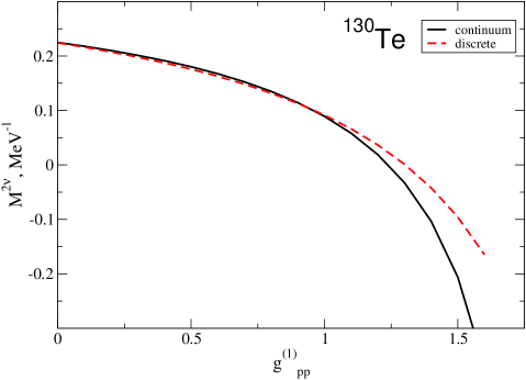
Figure 1: The calculated $g^{1}_{pp}$-dependence of $M^{2\nu}$ in both discretized and continuum QRPA.

The calculated values of $M^{0\nu}$ are given in Table I for both versions of the QRPA and $g_{A}=1.25$. Note that the two-nucleon short-range correlations are included in the calculations in terms of the Jastrow function. At the same time, the higher order terms of the nucleon current are not considered (they usually reduce $M^{0\nu}$ by about 30%, see, e.g. [2]).

The contributions of the multipoles up to $J^{\pi}=6^{-}$ ($L=0\div 5$) are included in the calculations of $M^{0\nu}$. Note that the QRPA itself as a long-wave approximation is barely suitable to describe the multipole contributions with $L>5$ (they contribute in total about 10% to $M^{0\nu}$), they are completely dominated by the short-range behavior of the wave function. The partial multipole contributions to the calculated $M^{0\nu}$’s are given in Fig. 2.

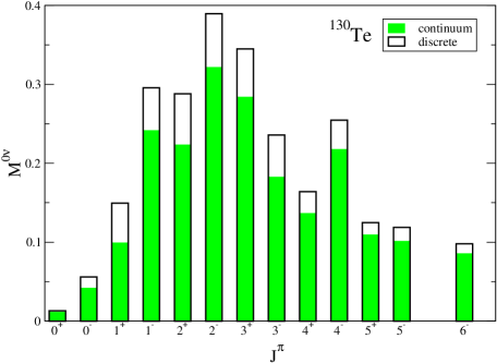
Figure 2: Multipole decomposition of $M^{0\nu}$ calculated within the both versions of the QRPA. $J^{\pi}$ is the angular momentum and parity of the intermediate states.

4 Conclusions

In the article a continuum-QRPA approach to calculation of $2\nu\beta\beta$- and $0\nu\beta\beta$-amplitudes has been formulated. For ¹³⁰Te a regular suppression (about 20%) of the $(L\geq 2)$-multipole contributons to $M^{0\nu}$ has been found which can be associated with additional ground state correlations appearing from the transitions to collective states in the continuum. At the same time the total $M^{0\nu}$ for ¹³⁰Te gets suppressed by about 20% as compared to the result of the discretized QRPA. As the nearest perspective we are going to perform a systematic analysis of other double-decaying nuclei within the cQRPA.

Acknowledgments

The work is supported in part by the Deutsche Forschungsgemeinschaft (grant FA67/28-2) and by the EU ILIAS project (contract RII3-CT-2004-506222).

References

• [1] V.A. Rodin, A. Faessler, F. Šimkovic and P. Vogel, Phys. Rev. C 68 (2003) 044302 .
• [2] V. A. Rodin, A. Faessler, F. Simkovic and P. Vogel, Nucl. Phys. A 766 (2006) 107 .
• [3] V.A. Rodin, M.H. Urin, A. Faessler, Nucl. Phys. A 747 (2005) 297 .
• [4] I.N. Borzov, E.L. Trykov, and S.A. Fayans, Sov. J. Nucl. Phys. 52 (1990) 627 ; I.N. Borzov, S.A. Fayans, and E.L. Trykov, Nucl. Phys. A 584 (1995) 335 ; I.N. Borzov and S. Goriely, Phys. Rev. C 62 (2000) 035501 .
• [5] V.A. Rodin and M.H. Urin, Phys. At. Nuclei 66 (2003) 2128 , nucl-th/0201065.
• [6] A. Faessler and F. Šimkovic, J. Phys. G 24 (1998) 2139 .
• [7] A.B. Migdal, Theory of finite Fermi-systems and properties of atomic nuclei (Moscow, Nauka, 1983) (in Russian).
• [8] P. Vogel and M.R. Zirnbauer, Phys. Rev. Lett. 57 (1986) 3148 .
• [9] J. Engel, P. Vogel and M. R. Zirnbauer, Phys. Rev. C 37 (1988) 731 .