Neutron star properties and the equation of state
of neutron-rich matter

Abstract

We calculate total masses and radii of neutron stars (NS) for pure neutron matter and nuclear matter in $\beta$-equilibrium. We apply a relativistic nuclear matter equation of state (EOS) derived from Dirac-Brueckner-Hartree-Fock (DBHF) calculations. We use realistic nucleon-nucleon (NN) interactions defined in the framework of the meson exchange potential models. Our results are compared with other theoretical predictions and recent observational data. Suggestions for further study are discussed.

1 Introduction

One of the most important and challenging problems in both theoretical and experimental nuclear physics is to understand the properties of matter under extreme conditions of density and pressure. The determination of the EOS (namely, the relationship between pressure and density) associated with such matter is a non-trivial problem which has attracted significant effort over the last few decades. Concerning terrestrial systems, detailed knowledge of the EOS is important, for instance, for understanding heavy-ion collision dynamics. On the other hand, the EOS is crucial for determining the properties of one of the most exotic objects in the universe–neutron stars. Neutron star properties depend on the knowledge of the EOS over a wide range of densities – from the density of iron at the stellar surface up to several times the density of normal nuclear matter in the core region of the star Weber99 .

Neutron stars are the smallest and densest stars known to exist. Like all stars neutron stars rotate–some at a rate of a few hundred revolutions per second. Such a fast rotating object will experience enormous centrifugal force which must be balanced by another force, gravity in this case, to prevent the star from falling apart. The balance of the two forces sets the lower limit on the stellar density Glendenning . Some neutron stars are in binary orbit with a companion and, in some cases, the application of orbital dynamics allows for an assessment of the masses. So far six neutron star binaries are known and all of them have masses in the range $1.36\pm 0.08M_{\odot}$ Thorsett&Chakrabarty . Clearly, observations of NS masses and radii impose important constraints on the EOS of dense matter, as the latter constitutes the basic input quantity that enters the structure equations of a neutron star Weber99 ; Wang ; Shapiro83 .

Although considerable progress has been made, the EOS of dense matter remains uncertain at densities above $\rho_{n}\simeq 3\times 10^{14}g/cm^{3}$ Ostgaard . For the reason stated above, this places uncertainty on the calculated NS properties. Determining the high density stellar matter EOS is a tremendous task. While at densities $\rho\simeq\rho_{0}$, ($\rho_{0}\simeq 0.17fm^{-3}$ is the normal nuclear density), matter consists mainly of nucleons and leptons, at higher densities several other species of particles are expected to appear due to the rapid rise of the baryon chemical potentials with density Baldo&Burgio2000 . Among these are strange baryons, such as the $\Lambda$, $\Sigma$, and $\Xi$ hyperons. In addition, pion-nucleon resonances may appear in stellar matter along with pion and kaon condensations. Moreover, at super high densities nuclear matter is expected to undergo a transition to quark-gluon plasma. The value of the transition density may be obtained from QCD lattice calculations at finite baryon densities, but is presently still uncertain Baldo&Burgio2000 .

After the first theoretical calculations of neutron star properties performed by Oppenheimer and Volkoff Oppenheimer&Volkoff39 and independently by Tolman Tolman39 , many theoretical predictions appeared in literature. Non-relativistic and relativistic approaches have been used. A number of early theoretical investigations on NS properties were done within the non-relativistic Skyrme framework. The reader is referred to the work of F. Douchin and P. Haensel in Ref. Douchin&Haensel01 . The conventional Brueckner theory with a continuous choice for the single particle potential and three-body forces was applied in Ref. Baldo&Burgio98 . Numerous predictions allow for hyperons together with nucleons and leptons in generalized $\beta$-equilibrium to be included in the stellar interior. The Brueckner-Hartree-Fock (BHF) scheme was extended to include these contributions Baldo&Burgio&Schulze98 ; Schulze98 and applied in NS calculations Baldo&Burgio2000 . Since the Walecka model Walecka86 was proposed and applied to nuclear matter properties, the relativistic mean field approach has been widely used in determining NS total masses and radii Li2004 ; Lawley2004 . The DBHF approach was used to compute NS properties in Refs. Ostgaard ; Sumiyoshi95 .

In general, the EOS of stellar matter is considerably model dependent and, as a result, predictions of NS properties are quite different from model to model. Among the sources of model dependence are Weber99 : (1) the many-body framework used for the determination of the EOS, (2) the model used for the bare NN interaction, (3) the kinds of hadrons/leptons included in the description of electrically neutral NS matter, (4) the treatment of pion and kaon condensations, (5) including the effects of fast rotation, (6) allowing for a phase transition from confined hadronic matter to deconfined quark matter. The possibility of such transition has attracted great interest over the last 30 years QM1 ; QM2 ; QM3 ; QM4 . It is generally agreed upon that the high pressure found in the core of a neutron star creates an ideal physical environment for hadrons to transform into quark matter – a state of matter of practically infinite lifetime. Nevertheless, until recently no empirical evidence had been reported. To a certain extent, this may signify that the occurrence (or not) of a transition to quark matter in the NS interior has only a minor impact on the overall static properties (range of possible masses, radii, limiting rotational periods) of the star Weber99 . The situation, however, could be completely different for the timing structure of a pulsar (its braking behavior as it evolves) which is expected to diverge significantly from the normal pulsar behavior if the star converts a fraction of its core matter to pure quark matter Weber99 .

Recently we have been concerned with probing the behavior of the isospin-asymmetric EOS Alonso&Sammarruca1 . In our work on neutron skins Alonso&Sammarruca2 , we have studied applications of the EOS at densities typical for normal nuclei. In Ref. SBK we discussed the one-body potentials for protons and neutrons from DBHF calculations of neutron rich matter (in particular their dependence upon the degree of asymmetry in proton and neutron concentrations). More recently, we applied our microscopic approach in calculations of effective in-medium NN cross sections SK . It is also important and timely to look into systems which are likely to constrain the behavior of the EOS at higher densities, where the largest model dependence is observed. This is the main purpose of the present paper, where we report predictions for masses and radii of static (non-rotating) neutron stars. Aside from minor adjustments, the framework is the one described in Ref. Alonso&Sammarruca1 . We apply a relativistic (DBHF-based) EOS and perform our calculations for two distinct cases: (1) pure neutron matter, and (2) baryon/lepton matter in $\beta$-equilibrium. It is also our objective to provide an overview of the present status of both theory and experimental constraints. Together with systematic calculations based on our microscopic model, this broad outlook will help us gauge the quality of our tools and determine the importance of potentially missing mechanisms.

This work is organized in the following way: after the introductory notes in this section, we briefly review our theoretical framework (section 2); the relativistic (DBHF-based) EOS for both neutron matter and $\beta$-stable matter is discussed in section 3; our numerical results are presented and discussed in section 4; we conclude in section 5 with a short summary and suggestions for further studies.

2 Formalism

In order to provide the reader with a self-contained manuscript, in this section we outline briefly the formalism used to derive the isospin-asymmetric EOS. A more extensive discussion can be found in Ref. Alonso&Sammarruca1 and references therein.

2.1 Realistic nucleon-nucleon interactions

The starting point of any microscopic calculation of nuclear structure or reactions is a realistic free-space NN interaction. A realistic and quantitative model for the nuclear force that has a reasonable basis in theory is the one-boson-exchange (OBE) model Machleidt89 . In this framework bosons with masses below the nucleon mass are typically included. The model we apply in the present study consists of six bosons four of which are of major importance: (1) The pseudoscalar pion with a mass of about 138 MeV. It is the lightest meson and provides the long-range part of the NN potential and most of the tensor force; (2) The $\rho$ vector meson – a $2\pi$ P-wave resonance with a mass of about 770 MeV and spin 1. Its major role is to cut down the pion tensor force at short range; (3) The $\omega$ vector meson – a $3\pi$ resonance of about 783 MeV and spin 1. It creates a strong repulsive central force of short range and the short-ranged spin-orbit force; (4) The isoscalar-scalar $\sigma$ boson with a mass of about 550 MeV. It provides the intermediate range attraction necessary for nuclear binding and can be understood as a simulation of the correlated S-wave $2\pi$-exchange.

The mesons are coupled to the nucleon through the following meson-nucleon Lagrangians for the pseudoscalar (ps), scalar (s), and vector ($\upsilon$) fields, respectively:

$${\cal{L}}_{p\upsilon}=-\frac{f_{ps}}{m_{ps}}\bar{\psi}\gamma^{5}\gamma^{\mu}\psi\partial_{\mu}\phi^{(ps)}$$ (1)

$${\cal{L}}_{s}=g_{s}\bar{\psi}\psi\phi^{(s)}$$ (2)

$${\cal{L}}_{\upsilon}=-g_{\upsilon}\bar{\psi}\gamma^{\mu}\phi_{\mu}^{(\upsilon)}-\frac{f_{\upsilon}}{4m}\bar{\psi}\sigma^{\mu\nu}\psi(\partial_{\mu}\phi^{(\upsilon)}_{\nu}-\partial_{\nu}\phi^{(\upsilon)}_{\mu})$$ (3)

with $\psi$ the nucleon and $\phi_{\mu}^{(\alpha)}$ the meson fields respectively (notation and conventions as in Ref. Bjorken&Drell ). For isovector (isospin 1) mesons (such as $\rho$ and $\pi$), $\psi^{(\alpha)}$ is to be replaced by $\tau\cdot\phi^{(\alpha)}$, with $\tau$ the usual Pauli matrices.

From the above Lagrangians the OBE amplitudes can be derived (see, for instance, Ref. Machleidt89 ). The OBE potential is defined as the sum of the OBE amplitudes of all exchanged mesons.

In this work, we use the Bonn A, B, and C parameterizations of the OBE potential formulated in the framework of the Thompson equation. The main difference between these three potentials is in the strength of the tensor force as reflected in the predicted D-state probability of the deuteron, $P_{D}$ Brockmann&Machleidt96 . Bonn A has the weakest tensor force with $P_{D}=4.5\%$ (see Table 2 in Ref. Brockmann&Machleidt96 ). The Bonn B and C potentials predict 5.1% and 5.5%, respectively. It is well known that the strength of the tensor force is a crucial factor in determining the location of the nuclear matter saturation point on the Coester band Coester .

2.2 Conventional Brueckner Theory

We review here the main steps leading to the self-consistent calculation of the energy per particle in infinite nuclear matter, with or without isospin asymmetry, within the BHF approach. This is mainly to provide a baseline for the next subsection where we describe its relativistic extension (which is the method we actually apply). For a complete description of the BHF method the reader is referred to Refs. Bethe71 ; Haftel&Tabakin70 ; Sprung72 . For a review, see, for example, Ref. Machleidt89 .

Nuclear matter is characterized by its total density or Fermi momentum $k_{F}$ (and the degree of isospin asymmetry, in case of unequal proton and neutron densities). With $k_{1}$ and $k_{2}$ being the momenta of two nucleons with respect to nuclear matter, it is customary to formulate the problem in terms of their relative momentum, ${\bf{K}}=\frac{1}{2}({\bf{k}}_{1}-{\bf{k}}_{2})$, and one-half of the center-of-mass momentum, ${\bf{P}}=\frac{1}{2}({\bf{k}}_{1}+{\bf{k}}_{2})$. (Clearly, ${\bf{k}}_{1,2}={\bf{P}}\pm{\bf{K}}$.)

The effective nucleon-nucleon interaction in nuclear matter is described in terms of the reaction matrix, or the Brueckner $G$-matrix, which satisfies the in-medium scattering equation (the Bethe-Goldstone equation)

$$G_{ij}({\bf{P;K,K_{0}}}) = V_{ij}({\bf{K,K_{0}}})-\int\frac{d^{3}K^{\prime}}{(2\pi)^{3}}V_{ij}({\bf{K,K^{\prime}}})$$ (4)

$$\times\frac{Q_{ij}({\bf{K^{\prime},P}};k_{F})G_{ij}({\bf{P;K^{\prime},K_{0}}})}{\epsilon_{ij}^{*}({\bf{P,K^{\prime}}})-(\epsilon_{ij}^{*})_{0}({\bf{P,K_{0}}})}$$

where $ij$=$nn$, $pp$, or $np$, and the asterisk signifies that medium effects are applied to these quantities. $\bf{K_{0}}$, $\bf{K}$, and $\bf{K^{\prime}}$ are the initial, final, and the intermediate momenta, respectively. $V_{ij}$ is the two body OBE potential briefly discussed in the previous subsection. $\epsilon_{ij}^{*}$ is the energy of the two-nucleon system, and $(\epsilon_{ij}^{*})_{0}$ is the starting energy. Thus,

$$\epsilon_{ij}^{*}({\bf{P,K}})=e_{i}^{*}({\bf{P,K}})+e_{j}^{*}({\bf{P,K}}),$$ (5)

with $e_{i,j}^{*}$ the total energy of a single nucleon in nuclear matter.

The $G$-matrix equation (Eq. (4)) is density dependent due to the presence of the Pauli projection operator, Q, which prevents scattering into occupied states and is defined as

$$Q_{ij}({\mathbf{K,P}},k_{F})=\left\{\begin{array}[]{l l}1&\quad\mbox{if $k_{1}>k_{F}^{i}$ and $k_{2}>k_{F}^{j}$}\\ 0&\quad\mbox{otherwise.}\end{array}\right.$$ (6)

Detailed expressions for the (angle-averaged) Pauli operator can be found, for instance, in Ref. Alonso&Sammarruca1 for the case of unequal proton and neutron Fermi momenta.

Equation (4) is density dependent also through the single-particle energy,

$$e_{i}^{*}=T_{i}(p)+U_{i}(p),$$ (7)

with $T_{i}(p)$ the kinetic energy and $U_{i}(p)$ the potential energy due to the interaction of the nucleon with all the others in the medium. We define

$$U_{i}(p)=<p|U_{i}|p> = Re[\sum_{q\leq k_{F}^{n}}<pq|G_{in}|pq-qp>$$ (8)

$$+\sum_{p\leq k_{F}^{p}}<pq|G_{ip}|pq-qp>]$$

with $|p>$ and $|q>$ single particle momentum, spin, and isospin states. Schematically, Eq. (8) has the form

$$U_{n}=U_{nn}+U_{np}$$ (9)

$$U_{p}=U_{pp}+U_{pn},$$ (10)

for neutrons and protons, respectively. Together with the $G$-matrix equation, Eqs. (9-10) constitute a coupled, self-consistency problem, which is solved using the “effective mass approximation” Haftel&Tabakin70 .

To demonstrate the self-consistency procedure, we take the non-relativistic single-particle energy Haftel&Tabakin70 and set

$$\frac{p_{i}^{2}}{2m_{i}}+U_{i}(p_{i})=\frac{p_{i}^{2}}{2m_{i}^{*}}+U_{0,i},$$ (11)

which amounts to parametrizing the potential $U_{i}(p)$ in terms of the nucleon effective mass $m_{i}^{*}$ and the constant $U_{0,i}$ ($i=n,p$). Equation (11) implies

$$U_{i}(p)=\frac{1}{2}\frac{m_{i}-m_{i}^{*}}{m_{i}m_{i}^{*}}p^{2}+U_{0,i}.$$ (12)

Hence in the non-relativistic case the single-particle potential, $U_{i}(p)$, has been fitted with a quadratic function of $p$. (The subscript “$i$” signifies that the parameters are different for neutrons and protons.) Starting with some initial values of $m_{i}^{*}$ and $U_{0,i}$, the $G$-matrix equation is solved and a first solution for $U_{i}(p)$ is obtained. These solutions are then parameterized in terms of a new set of constants, and the procedure is repeated until convergence is reached (that is, until differences between the parameters from successive iterations are within the desired accuracy). Once the single-particle potential is available, we calculate the (average) energy per particle (to lowest order in the $G$-matrix).

As is well known, nuclear matter calculations based on the BHF approach fail to predict correctly the saturation properties of nuclear matter. The typical trend is that the saturation density is too high for reasonable energies. Different calculations based on the conventional BHF approach differ somewhat in their predictions of nuclear matter saturation properties, but all of them fail to predict simultaneously the correct saturation energy and density Machleidt89 . For this reason, it has become popular to implement non-relativistic calculations with contributions from phenomenological three-body forces.

On the other hand, already more than two decades ago it was realized that the explicit treatment of the lower component of the Dirac spinor in the medium could provide the missing saturation mechanism. This observation started what became known as the DBHF approach. We review some of the main points in the next section.

2.3 The Dirac-Brueckner-Hartree-Fock approach

For a detailed description see, for example, Refs. Brockmann&Machleidt90 ; Horowitz&Serot84 ; Haar&Malfleit87 . The essential point of the DBHF approach is to use the Dirac equation for the single particle motion in nuclear matter

$$(\not{p}_{i}-m_{i}-U_{i}(p))u_{i}({\bf{p}},s)=0,$$ (13)

where the most general Lorentz structure for $U_{i}(p)$ is approximated as Brockmann&Machleidt90

$$U_{i}(p)\approx U_{S,i}(p)+\gamma_{0}U^{0}_{V,i}(p).$$ (14)

Here $U_{S,i}$ is an attractive scalar field and $U^{0}_{V,i}$ is the timelike component of a repulsive vector field. The fields $U_{S,i}$ and $U^{0}_{V,i}$ are in the order of several hundred MeV and strongly density dependent Brockmann2000 . With the definitions $m_{i}^{*}(p)=m_{i}+U_{S,i}(p)$ and $(p_{i}^{0})^{*}=p_{i}^{0}-U^{0}_{V,i}(p)$, the Dirac equation in nuclear matter can be written as

$$(\not{p}_{i}^{*}-m_{i}^{*})u_{i}({\bf{p}},s)=0.$$ (15)

The positive energy solution of Eq. (15) is given by

$$u_{i}({\bf{p}},s)=\left(\frac{E_{i}^{*}(p)+m_{i}^{*}}{2m_{i}^{*}}\right)^{1/2}\left(\begin{array}[]{c}1\\ \frac{\sigma\cdot{\bf{p}}}{E_{p,i}^{*}+m_{i}^{*}}\end{array}\right)\chi_{S},$$ (16)

with $\chi_{S}$ a Pauli spinor, and $E_{i}^{*}(p)=(m_{i}^{*}{{}^{2}}+{\bf{p}}^{2})^{1/2}$. We notice that this is formally identical to the free-space spinor, but with $m_{i}$ replaced by $m_{i}^{*}$.

The single particle potential is then calculated from the operator given in Eq. (14) and properly normalized Dirac spinors. Namely,

$$U_{i}(p)=\frac{m_{i}^{*}}{E_{i}^{*}}<p|U_{S,i}(p)+\gamma^{0}U_{V,i}^{0}(p)|p>.$$ (17)

The quantities $U_{S,i}$ and $U_{V,i}^{0}$ are momentum dependent, but to a good approximation can be taken as constant Brockmann&Machleidt90 ; Haar&Malfleit87 . Hence, for the single particle potential, one can write

$$U_{i}(p)=\frac{m_{i}^{*}}{E_{i}^{*}(p)}U_{S,i}+U^{0}_{V,i},$$ (18)

which, as in Eq. (12), again amounts to parameterizing the single particle potential in terms of two constant quantities (for each type of nucleon). In analogy with the usual Hartree-Fock definition of the single particle potential (see Eq. (8)), we also write

$$U_{i}(p) = Re[\sum_{q\leq k_{F}^{n}}\frac{m_{i}^{*}m_{n}^{*}}{E_{i}^{*}(p)E_{n}^{*}(q)}<pq|g_{in}|pq-qp>$$ (19)

$$+\sum_{q\leq k_{F}^{p}}\frac{m_{i}^{*}m_{p}^{*}}{E_{i}^{*}(p)E_{n}^{*}(q)}<pq|g_{ip}|pq-qp>]$$

where $g_{ij}$ satisfies the relativistic scattering equation

$$g_{ij}({\bf{P,K,K_{0}}})=\upsilon_{ij}^{*}({\bf{K,K_{0}}})-\int\frac{d^{3}K^{\prime}}{(2\pi)^{3}}\upsilon_{ij}^{*}({\bf{K,K^{\prime}}})\frac{m_{i}^{*}m_{j}^{*}}{E_{i}^{*}E_{j}^{*}}\frac{Q_{ij}({\bf{K^{\prime},P}};k_{F})g_{ij}({\bf{P;K^{\prime},K_{0}}})}{\epsilon_{ij}^{*}({\bf{P,K^{\prime}}})-(\epsilon_{ij}^{*})_{0}({\bf{P,K_{0}}})}.$$ (20)

Using the definitions $G_{ij}=\frac{m_{i}^{*}}{E_{i}^{*}}g_{ij}\frac{m_{j}^{*}}{E_{j}^{*}}$ and $V_{ij}^{*}=\frac{m_{i}^{*}}{E_{i}^{*}}\upsilon_{ij}^{*}\frac{m_{j}^{*}}{E_{j}^{*}}$, Eq. (20) can be rewritten as

$$G_{ij}({\bf{P;K,K_{0}}})=V_{ij}^{*}({\bf{K,K_{0}}})-\int\frac{d^{3}K^{\prime}}{(2\pi)^{3}}V_{ij}^{*}({\bf{K,K^{\prime}}})\frac{Q_{ij}({\bf{K^{\prime},P}};k_{F})G_{ij}({\bf{P;K^{\prime},K_{0}}})}{\epsilon_{ij}^{*}({\bf{P,K^{\prime}}})-(\epsilon_{ij}^{*})_{0}({\bf{P,K_{0}}})},$$ (21)

which is formally identical to the non-relativistic $G$-matrix equation (Eq. (4)). We are then in a situation that is technically equivalent to the non-relativistic case, except for the Dirac structure of the single-particle energy. Namely, Eqs. (19) and (21) (where the potential $V_{ij}^{*}$ is written in terms of in-medium spinors, Eq. (16)), must be solved self-consistently for $G_{ij}$ and the single particle potential, $U_{i}(p)$, with the help of the chosen parametrization, Eq. (18). We then proceed to calculate the energy per particle.

In summary, the most significant difference between the BHF and DBHF schemes is that in the latter case the nucleon wave function is obtained self-consistently, while in the BHF approach the free-space solution is used. This difference turns out to be an important one – as a result of the reduced nucleon mass in the medium, the lower component of the nucleon spinor is larger than in free space. This is well known to produce a density-dependent, repulsive-many body effect, with the result that the predicted saturation density and energy are consistent with the empirical values Brockmann&Machleidt90 . Physically, the description of the nucleon in nuclear matter with a Dirac spinor as in Eq. (16) can be regarded as effectively taking into account some many-body force contributions 3B (hence, the reduced need for inclusion of three-body forces in the relativistic scheme).

2.4 Relativistic stellar structure equations

In the present section we discuss the structure equations of static (non-rotating) neutron stars. These are objects of highly compressed matter so that the geometry of spacetime is changed considerably from that of flat space. Thus models of such stars need to be constructed within the framework of General Relativity combined with theories of superdense matter. The connection between these two branches of physics is provided by Einstein’s field equations

$$G^{\mu\nu}=8\pi GT^{\mu\nu}(\epsilon,P(\epsilon)),$$ (22)

which couple the Einstein curvature tensor, $G^{\mu\nu}$, to the energy-momentum density tensor, $T^{\mu\nu}$, of stellar matter. The tensor $T^{\mu\nu}$ contains the equation of state in the form $P(\epsilon)$ (pressure, $P$, as a function of the energy density, $\epsilon$), and $G$ is the gravitational constant.

Einstein’s field equations are completely general and simple in appearance. However they are exceedingly complicated to solve because of their non-linear character and because spacetime and matter act upon each other. There are only a few cases in which solutions can be found in closed form. One of the most important closed-form solutions is the Schwarzschild metric outside a spherical star. Another is the Kerr metric outside a rotating black hole.

Starting from Einstein’s field equations one can derive the structure equations of a static, spherically symmetric, relativistic star. For an explicit treatment and derivation see for example the work of Fridolin Weber in Ref. Weber99 . These equations are generally known as Tolman-Oppenheimer-Volkoff (TOV) equations. In a system of units where $c=G=1$, the TOV equations can be written as

$$\frac{dP}{dr} = -\frac{\epsilon(r)m(r)}{r^{2}}\left[1+\frac{P(r)}{\epsilon(r)}\right]$$ (23)

$$\times\left[1+\frac{4\pi{r^{3}}P(r)}{m(r)}\right]\left[1-\frac{2m(r)}{r}\right]^{-1}$$

$$\frac{dm(r)}{dr}=4\pi\epsilon(r)r^{2}dr.$$ (24)

To proceed to the solution of these equations, it is necessary to provide the EOS of stellar matter in the form $P(\epsilon)$. Starting from some central energy density $\epsilon_{c}=\epsilon(0)$ at the center of the star $(r=0)$, and with the initial condition $m(0)=0$, the above equations can be integrated outward until the pressure vanishes, signifying that the stellar edge is reached. Some care should be taken at $r=0$ since, as seen above, the TOV equations are singular there. The point $r=R$ where the pressure vanishes defines the the radius of the star and $M=m(R)=4\pi\int_{0}^{R}\epsilon(r^{\prime})r^{\prime 2}dr^{\prime}$ its gravitational mass.

For a given EOS, there is a unique relationship between the stellar mass and the central density $\epsilon_{c}$. Thus, for a particular EOS, there is a unique sequence of stars parameterized by the central density (or equivalently the central pressure $P(0)$).

In this work we apply a standard fifth order Runge-Kutta numerical scheme NR to integrate the TOV equations, which are supplemented by the EOS in numerical form. In the next section, we discuss the features of the EOS applied in this study.

3 Equation of state

We apply here the relativistic equation of state. For a detailed discussion of the isospin-dependent EOS we refer the reader to Ref. Alonso&Sammarruca1 . In the present study we calculate neutron star properties considering either pure neutron matter or asymmetric matter in $\beta$-equilibrium.

3.1 Neutron matter EOS

The degree of isospin asymmetry is represented by the asymmetry parameter, $\alpha=\frac{\rho_{n}-\rho_{p}}{\rho}$ with $\rho_{n,p}$ the neutron/proton densities and $\rho=\rho_{n}+\rho_{p}$ the total density. (Clearly, $\alpha=0$ for symmetric nuclear matter and $\alpha=1$ for pure neutron matter.) The isopsin-dependent EOS can be written as Alonso&Sammarruca1

$$\bar{e}(k_{F},\alpha)=\frac{(1+\alpha)\bar{e}_{n}+(1-\alpha)\bar{e}_{p}}{2}$$ (25)

with $\bar{e}_{n,p}$ the average energy per neutron/proton and $\bar{e}(k_{F},\alpha)$ the energy per particle as a function of the total Fermi momentum and the asymmetry parameter. The total Fermi momentum, $k_{F}$, is related to the total density, $\rho$, in the usual way

$$\rho=\frac{2k_{F}^{3}}{3\pi^{2}}.$$ (26)

We start with showing the isospin-dependent EOS for neutron and symmetric matter, see Fig. 1. In both cases, predictions are shown for DBHF and BHF calculations and all three NN potentials referred to in subsection 2.1. For the case of pure neutron matter (upper frame of Fig. 1), we see essentially no differences among the predictions from the three potentials. As already discussed, a main source of differences among the three versions of the Bonn potential is in the strength of the tensor force, which is mostly reflected in the ($T=0$) ${}^{3}S_{1}-^{3}D_{1}$ coupled states. In neutron matter ($T=1$), however, this partial wave does not contribute and thus the model dependence is dramatically reduced Li92 . Consistent with these observations, in symmetric matter significant differences are observed among the three potentials, see lower panel of Fig. 1. Notice that our EOSs are considerably more attractive than those shown in Ref. Machleidt89 and also calculated with Bonn A, B, and C. For details on the differences between our respective calculations we refer the reader to Ref. Alonso&Sammarruca2 .

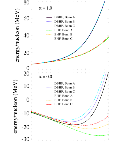
Figure 1: (Color online) EOS for neutron ($\alpha=1.0$) and symmetric matter ($\alpha=0.0$).

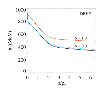
Figure 2: (Color online) Effective nucleon masses in neutron ($\alpha=1.0$) and symmetric ($\alpha=0.0$) matter as a function of density. For $\alpha=0.0$, the solid (black), dotted (dark blue), and dashed (light blue) curves correspond to Bonn A, B, and C, respectively. No differences can be seen among the predictions from the three potentials in the case of neutron matter.

For solving the TOV equations one needs to compute energy density and pressure, both of which are simply related to the EOS. As previously outlined, in our self-consistent calculation of the EOS we fit the single-particle potential with its “effective mass approximation”. Although chosen on reasonable theoretical grounds, the ansatz we use has a finite domain of validity (for which reliable convergenge of the self-consistent procedure can be obtained.) On the other hand, for NS calculations one needs to supply the relationship between energy density and pressure over a very wide range of densities. The EOS at the lowest/highest densities have been derived with different methods, usually coupling available parametrizations of different EOSs Ostgaard ; Sumiyoshi95 . Here, in the effort of keeping internal consistency as far as possible, we first obtain nucleon effective masses by interpolating the available predictions to the free-space value (to cover the small low-density part, approximately $\rho<0.03$ fm^-3) and extrapolating to the higher densities (approximately $\rho>0.6$ fm^-3). With the masses thus generated, we then proceed to the usual (microscopic) calculation of the energy per particle everywhere in the needed range. (Notice that the calculation of the $G$-matrix, and ultimately of the energy/particle, can proceed as long as effective masses are provided, as the momentum-independent part of the single-nucleon potential in Eq. (18) (or Eq. (12)) drops out from the energy denominator in Eq. (4).)

The effective masses are shown in Fig. 2 for both symmetric and neutron matter. We note the weaker density dependence at the higher densities, a behavior that is already reflected in the self-consistent calculation and appears reasonable on physical grounds. The nucleon effective masses originate from the (attractive) scalar potential in the Dirac equation, which, in turn, is sensitive mostly to the scalar meson $\sigma$. As density increases, short-range contributions become dominant over intermediate-range attraction. This results into the observed lesser sensitivity of the effective masses to increasing density. (Further discussion on the high-density behavior of EOS will be presented in subsection 3.3.)

The energy density, $\epsilon$, is defined as

$$\epsilon(\rho,\alpha)=\rho[\bar{e}(\rho,\alpha)+m_{N}^{free}]$$ (27)

where $\bar{e}(\alpha,\rho)$ is the energy per nucleon and $m_{N}^{free}$ is the nucleon rest mass. The pressure in nuclear matter is defined in terms of the energy per particle and the baryon number density as

$$P(\rho,\alpha)=\rho^{2}\frac{\partial\bar{e}(\rho,\alpha)}{\partial\rho}.$$ (28)

In the upper frame of Fig. 3 we show the energy density, $\epsilon$, as a function of the baryon number density, $\rho$, calculated with the Bonn A, B, and C potentials. The pressure, $P$, as a function of $\rho$ is shown in the lower panel of Fig. 3. We also note that our predictions are reasonably consistent with most recent constraints on neutron and symmetric matter pressure obtained through medium energy heavy ion collisions MSU05 . For the reasons discussed earlier, hardly any model dependence is seen in the pure $T=1$ system. Accordingly, very small differences can be expected among the NS properties computed from pure neutron matter using the three potentials under consideration. (We reiterate that this is due to the relationship among these potentials in particular, and does not imply model independence in general.) Next we discuss the EOS for $\beta$-stable matter.

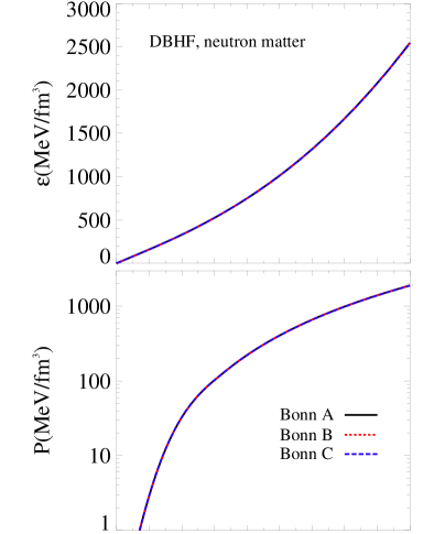
Figure 3: (Color online) EOS for pure neutron matter. The upper panel shows the energy density and the lower panel the pressure as a function of the baryon number density.

3.2 $\beta$-stable matter EOS

The density dependence of the symmetry energy determines the proton fraction in $\beta$-equilibrium, and, in turn, the cooling rate and neutrino emitting processes.

First, we consider a system of nucleons and electrons only. From the $\beta$-stability condition, the chemical potential of the electrons is written as

$$\mu_{n}-\mu_{p}=\mu_{e}$$ (29)

Deriving the EOS of $\beta$-stable matter requires knowing the corresponding proton fraction, $Y_{p}=\frac{\rho_{p}}{\rho}$. The equilibrium particle concentrations, $Y_{i}=\frac{\rho_{i}}{\rho}$ ($i=e$, $n$, $p$), can be calculated via Eq. (29) combined with the charge neutrality condition $\rho_{e}=\rho_{p}$ (i.e. $Y_{e}=Y_{p}$) and $\rho=\rho_{n}+\rho_{p}$ (i.e. $1=Y_{n}+Y_{p}$). To compute the various chemical potentials,

$$\mu_{i}=\frac{\partial e_{tot}}{\partial Y_{i}},$$ (30)

we write $e_{tot}$ as

$$e_{tot}(\rho,Y_{p},Y_{n},Y_{e})=\bar{e}(\rho,Y_{p})+\frac{\rho_{p}}{\rho}m_{p}c^{2}+\frac{\rho_{n}}{\rho}m_{n}c^{2}+\frac{E_{e}}{A}.$$ (31)

Here $\bar{e}(\rho,Y_{p})$ is the energy per nucleon and $\frac{E_{e}}{A}$ is the contribution to the total energy from the electrons. Similarly to what is done in Ref. Bombaci&Lombardo91 , we assume a simple model for electrons and treat them as a gas of extremely relativistic non-interacting fermions. That is, for electrons we set

$$c(p^{2}+m_{e}^{2}c^{2})^{1/2}\approx pc,$$ (32)

which appears reasonable since the electron mass $m_{e}$ is small compared to its chemical potential at typical nuclear density. Integrating over all momentum states (and summing over spin states), it is easy to show that the electron energy density (or energy per volume) becomes

$$\frac{E_{e}}{V}=\frac{(k_{F}^{e})^{4}}{4\pi^{2}}=\frac{(3\pi^{2}{\rho}Y_{e})^{4/3}}{4\pi^{2}}$$ (33)

where $k_{F}^{e}$ is the electron Fermi momentum.

In Ref. Alonso&Sammarruca1 we have verified that the energy per nucleon can be written as

$$\bar{e}(k_{F},\alpha)=\bar{e}(k_{F},0)+e_{sym}(k_{F})\alpha^{2},$$ (34)

with $\bar{e}(k_{F},0)$ the energy per particle for symmetric matter and $e_{sym}$ the symmetry energy defined by

$$e_{sym}(k_{F})=\left.\frac{1}{2}\frac{\partial^{2}\bar{e}(k_{F},\alpha)}{\partial^{2}\alpha}\ \right|_{\alpha=0}.$$ (35)

With the definition $\alpha=1-2Y_{p}$, Eq. (34) becomes

$$\bar{e}(\rho,Y_{p})=\bar{e}(\rho,Y_{p}=\frac{1}{2})+e_{sym}(\rho)(1-2Y_{p})^{2}.$$ (36)

Thus, $e_{tot}$ is written as

$$e_{tot}(\rho,Y_{p},Y_{n},Y_{e})=\bar{e}(\rho,Y_{p}=\frac{1}{2})+e_{sym}(\rho)(1-2Y_{p})^{2}$$

$$+Y_{p}m_{p}c^{2}+Y_{n}m_{n}c^{2}+\hbar c\frac{(3\pi^{2}Y_{e})^{4/3}}{4\pi^{2}}\rho^{1/3},$$ (37)

where the last therm can be obtained trivially from Eq. (33) divided by the density. Knowing the total energy allows one to evaluate the chemical potentials, which, in turn, are inserted in Eq. (29) (combined with the constraint $Y_{p}=Y_{e}$) to give a simple algebraic equation for $Y_{p}$

$$-4e_{sym}(\rho)(1-2Y_{p})+(m_{p}-m_{n})c^{2}+\hbar{c}(3\pi^{2}\rho)^{1/3}Y_{p}^{1/3}=0.$$ (38)

The solution of this equation is inserted in Eq. (36) to provide the EOS of nuclear matter in $\beta$-equilibrium with electrons.

Just above the density of normal nuclear matter, the electron chemical potential, $\mu_{e}$, exceeds the muon mass, $m_{\mu}$, and the reaction $n\leftrightarrow p+\mu^{-}$ becomes energetically allowed WFF88 . Under these circumstances the $\beta$-stability condition and charge-neutrality require

$$\mu_{e}=\mu_{\mu},$$ (39)

and

$$\rho_{p}=\rho_{e}+\rho_{\mu}$$ (40)

(and thus, $Y_{p}-Y_{e}-Y_{\mu}=0$). Equation (31) needs to be modified to include the muon contribution to the total energy,

$$e_{tot}(\rho,Y_{p},Y_{n},Y_{e},Y_{\mu}) = \bar{e}(\rho,Y_{p})+Y_{p}m_{p}c^{2}+Y_{n}m_{n}c^{2}$$ (41)

$$+ \frac{E_{e}}{A}+\frac{E_{\mu}}{A}.$$

We will treat muons as a gas of non-interacting nonrelativistic fermions MBBS04 , a reasonable approximation given the relatively large muon mass (compared to its Fermi momentum at typical muon concentrations in $\beta$-equilibrium). It can then be shown that the muon energy density is Glendenning

$$\frac{E_{\mu}}{V}\approx\rho_{\mu}m_{\mu}+\frac{(3\pi^{2}\rho_{\mu})^{5/3}}{10\pi^{2}m_{\mu}}$$ (42)

(in units where $c=\hbar=1$). Thus, Eq. (41) becomes

$$e_{tot}(\rho,Y_{p},Y_{n},Y_{e},Y_{\mu})=\bar{e}(\rho,Y_{p}=\frac{1}{2})+e_{sym}(\rho)(1-2Y_{p})^{2}$$

$$+Y_{p}m_{p}c^{2}+Y_{n}m_{n}c^{2}+{\hbar c}\frac{(3\pi^{2}Y_{e})^{4/3}}{4\pi^{2}}\rho^{1/3}$$

$$+Y_{\mu}m_{\mu}c^{2}+\frac{(\hbar c)^{2}}{2m_{\mu}c^{2}}\frac{(3\pi^{2}Y_{\mu})^{5/3}}{5\pi^{2}}\rho^{2/3},$$ (43)

where the muon contribution to the total energy per particle is obtained from Eq. (42) divided by $\rho$. As done in case of nucleons and electrons only, evaluating the chemical potentials, combined with Eqs. (39) and (40) leads to the following algebraic equations for the equilibrium particle concentrations ($Y_{i}$)

$$-4e_{sym}(\rho)(1-2Y_{p})+(m_{p}-m_{n})c^{2}+\hbar{c}(3\pi^{2}\rho)^{1/3}Y_{e}^{1/3}=0$$ (44)

$$m_{\mu}c^{2}+({\hbar}c)^{2}\frac{(3\pi^{2})^{5/3}}{6\pi^{2}m_{\mu}c^{2}}\rho^{2/3}Y_{\mu}^{2/3}-\hbar{c}(3\pi^{2}\rho)^{1/3}Y_{e}^{1/3}=0$$ (45)

$$Y_{p}-Y_{e}-Y_{\mu}=0.$$ (46)

Once $Y_{p}$ is obtained from the above equations, it is inserted in Eq. (36) to provide again the EOS of $\beta$-stable matter. The energy density of baryon/lepton matter in $\beta$-equilibrium is then used as the new input for the TOV equations.

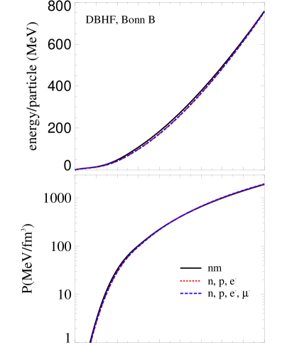
Figure 4: (Color online) EOS for neutron matter and baryon/lepton matter in $\beta$ equilibrium. Predictions are obtained with the Bonn B potential. The upper panel shows the energy density and the lower panel the pressure as a function of the baryon number density.

In Fig. 4 we compare EOSs for neutron matter and $\beta$-stable matter (for both $e^{-}$ and $e^{-}$ plus $\mu^{-}$ cases), obtained with the Bonn B potential. We observe only very small differences among the various predictions, although the $\beta$-stable EOSs are slightly “softer” than the one for pure neutron matter (at intermediate densities), a trend that is independent of the particular NN potential being used. This is to be expected, since a system with some $T$=0 component is generally more attractive (mostly through the ${}^{3}S_{1}$ partial wave) than a pure $T$=1 system. This point will be looked at more closely in the next subsection.

The symmetry energy and the proton fraction in $\beta$-stable matter are displayed in Fig. 5. We observe that the symmetry energy (upper frame) tends to saturate and eventually decreases with density, a behavior qualitatively similar to the one seen in the proton fraction (middle frame). From the lower panel of Fig. 5, we see that the addition of muons increases the proton fraction noticeably. In particular, the maximum proton fraction increases from 0.11 to about 0.13 (with Bonn B). We recall that a proton fraction larger than approximately $\frac{1}{9}$ would allow a critical cooling mechanism for the neutron star via the direct URCA processes LP2004 . On the other hand, due to the behavior of the predicted symmetry energy (the crucial player in the determination of the proton fraction), our proton concentrations remain very small, and thus the EOS is only mildly impacted by the inclusion of leptons. In Fig. 6 we show the different particle concentrations as a function of density. The presence of muons becomes possible only at higher densities, due to the energetic constraints mentioned earlier. Also, their concentration remains substantially below the electron fraction.

In closing this section, we stress that the high-density behavior of the symmetry energy is very poorly constrained and theoretically controversial, with different models often yielding dramatically different predictions. A more detailed discussion on this and related issues is presented next.

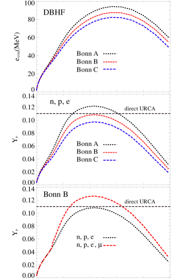
Figure 5: (Color online) Symmetry energy, $e_{sym}$, and proton fraction in $\beta$-equilibrium, $Y_{P}$. The upper panel shows the symmetry energy and the middle/lower panel the proton fraction as a function of density.

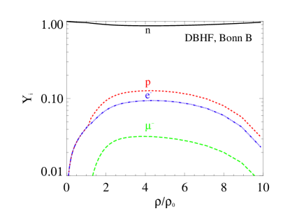
Figure 6: (Color online) Concentrations of various particle species ($Y_{i}=\rho_{i}/\rho$) in $\beta$-stable matter as a function of the baryon number density in units of $\rho_{0}$.

3.3 High-density equation of state and the meson model: further discussion

In this subsection, we take a more in-depth look at how the observed features of the EOS and the symmetry energy can be understood in relation to the physical components of our model.

First, we observe that from Eq. (34) one can write

$$\bar{e}(k_{F},\alpha=1)-\bar{e}(k_{F},\alpha=0)=e_{sym}(k_{F}),$$ (47)

which clearly displays the significance of the symmetry energy as the energy shift between neutron and symmetric matter. Thus, the behavior of $e_{sym}$ reflects the relationship between $\bar{e}(k_{F},\alpha=1)$ and $\bar{e}(k_{F},\alpha=0)$ as a function of density. What we observe in the present calculation is that the energy per particle in symmetric matter becomes more and more repulsive with increasing density, eventually approaching the one of neutron matter. Within the meson model, this can be understood in terms of the competing roles of the intermediate-range attraction (provided by the scalar meson $\sigma$ and the iterated one-pion exchange) and the short-range repulsion (generated by the vector meson $\omega$), as we describe next. Neutron matter is generally a more repulsive system because it lacks the contribution from T=0 waves, some of which are very attractive at normal nuclear densities (hence, for instance, the crucial role of the ${}^{3}S_{1}$ state in nuclear binding). On the other hand, as density increases, short-range repulsion becomes the dominant contribution to the NN interaction. Furthermore, in the DBHF calculations the (repulsive) spin-orbit interaction is strongly enhanced due to the relativistic effective mass in the OBE potential. Therefore, keeping in mind that only T=1 states contribute to the energy of neutron matter while both isospin states contribute to the energy of nuclear matter, if major T=0 partial waves become increasingly repulsive at short distances, it is possible for the energy of symmetric matter to grow at a faster rate and eventually approach the neutron matter EOS. This is just what we observe in our model, as can be seen from Fig. 7, where we compare the energy per particle in symmetric and neutron matter up to very high densities. (The arguments above also explain why the EOSs for neutron matter and $\beta$-stable matter are very close to each other, cf. Fig. 4.)

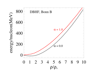
Figure 7: (Color online) Energy per nucleon for neutron (red curve) and symmetric (black curve) matter.

To explore this further as well as check internal consistency, we have performed some diagnostic tests. We find that the contributions to the average potential energy of symmetric matter from only ${}^{1}S_{0}$ are -18.75 MeV, -22.75 MeV, and 5.554 MeV at $k_{F}$=1.4, 2.0, and 2.5 fm^-1, respectively. Similarly, including only the ${}^{3}S_{1}$ and ${}^{3}D_{1}$ states, we find (for the same Fermi momenta) -18.74 MeV, -10.04 MeV, and 18.16 MeV. A correct way to state the result of the above tests is to say that, in the presence of repulsive forces only (a scenario simulated by the presence of high-density), nuclear matter would be a more repulsive system than neutron matter (for the same $k_{F}$).

At some critical density, signaled by the symmetry energy turning negative, it would then be possible for a pure neutron system to become more stable than symmetric matter, a phenomenon referred to as isospin separation instability Li02 . Clearly, the value of such critical density depends upon the relative degrees of attraction and repulsion in the particular model under consideration. (Figure 5 suggests that in the present model this would happen at densities well above ten times nuclear matter density.)

It is of course possible that contributions not included in our model would soften the EOS in such a way as to alter the balance between the curves shown in Fig. 7 and, in turn, the high-density behavior of the symmetry energy. This is precisely among the aspects we wish to learn about with this and future studies (namely, domain of validity of the meson-theoretic picture, density dependence of the repulsive core, etc…). Systematic calculations based not on phenomenology but on a consistent theoretical framework (in spite of its inherent limitations), together with stringent constraints, can help achieve that purpose. Our main conclusion at this point is that empirical constraints specifically on the high-density behavior of the symmetry energy would provide some clear and direct information on the short-range nature of the nuclear force.

4 Results for neutron star total masses and radii

In Fig. 8 we show the total masses and radii versus the stellar central density, $\rho_{c}$. As expected in the light of our previous discussion, the NS properties computed from the EOS of neutron matter are essentially the same for all of the three potentials applied here. Consistent with the observations contained in subsection 3.3, the $\beta$-stable matter EOS, being only slightly softer than the pure neutron matter EOS, yields similar predictions, although radii tend to be smaller at higher central densities. In summary the neutron matter EOS from DBHF calculations yields a maximum mass $M_{max}\simeq 2.25$ $M_{\odot}$ at radius $R\simeq 11.01$ km and central density $\rho_{c}\simeq 0.98$ $fm^{-3}$. The relativistic EOS for $\beta$-stable matter yields maximum masses in the range $M_{max}\approx(2.238-2.241)$ $M_{\odot}$ at radii $R\approx(10.74-10.87)$ km and central densities $\rho_{c}\approx(0.998-1.013)$ $fm^{-3}$. Including muons in the description of $\beta$-stable matter does not alter significantly the predicted NS properties from the electrons-only case. Table 1 provides an overview of our predictions. Figure 9 displays the mass-radius relation for the NS models shown in Fig. 8.

Before we proceed with our discussion, we recall (see section 3) that an extrapolation is applied to the nucleon effective mass at those densities where a self-consistent solution for the single-particle potential is not available. Of course, every numerical extrapolation/interpolation involves uncertainties of some degree. To investigate to what extent the NS properties are sensitive to variations of $m^{*}$, we have performed numerous tests all of which verify that the predicted NS masses and radii are not affected significantly by moderate variations of the nucleon effective mass. For instance, uncertainty of 20% in the high density effective mass results in approximately 2.9% variation in the NS maximum mass, 1.54% in the radius, and about 0.31% in the central density (e.g. Bonn B, DBHF, neutron matter: $M_{max}=2.2457\pm 0.0659M_{\odot}$, $R=11.001\pm 0.17$ km, $\rho_{c}=0.979\pm 0.003fm^{-3}$). Very similar conclusions apply for the case of $\beta$-stable matter. (Sensitivity tests are performed in the following way: the highest density mass in Fig. 2 is varied by up to 20% and the self-consistently calculated values are then joined to it by interpolation. In this way the applied mass variation increases gradually as we move to higher densities, where the uncertainty should be largest.)

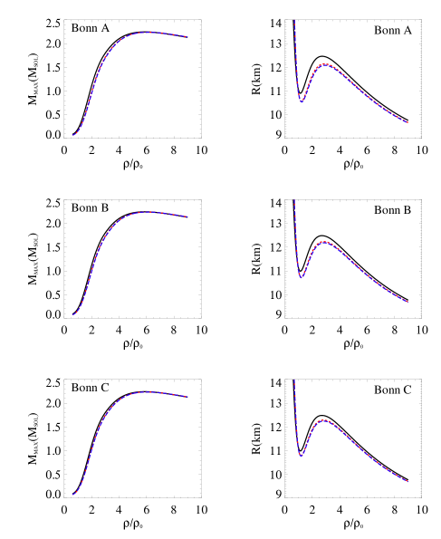
Figure 8: (Color online) NS total masses and radii. In all frames the solid (black) curve corresponds to the DBHF calculation for pure neutron matter, the short-dashed (red) curve to the DBHF calculation for $\beta$-stable matter of nucleons and electrons only, and the long-dashed (blue) curve to the DBHF calculation for nucleons, electrons and muons in $\beta$-equilibrium.

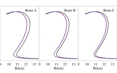
Figure 9: (Color online) Mass-radius relation. The curves are labeled as in Fig. 8.

Table 1: NS maximum masses, radii, and central densities (from DBHF calculations).

potential model	composition	$M_{max}(M_{\odot})$	$R(km)$	$\rho_{c}(fm^{-3})$
Bonn A	n	2.2456	11.00	0.979
Bonn B	n	2.2453	11.01	0.979
Bonn C	n	2.2439	11.02	0.978
Bonn A	n,p,$e^{-}$	2.2414	10.78	1.007
Bonn B	n,p,$e^{-}$	2.2413	10.83	1.002
Bonn C	n,p,$e^{-}$	2.2399	10.87	0.998
Bonn A	n,p,$e^{-},\mu^{-}$	2.2401	10.74	1.013
Bonn B	n,p,$e^{-},\mu^{-}$	2.2399	10.79	1.008
Bonn C	n,p,$e^{-},\mu^{-}$	2.2384	10.83	1.003

Our findings are generally consistent with previous ones obtained from similar theoretical frameworks Ostgaard ; Baldo&Burgio98 ; Sumiyoshi95 . In Ref. Ostgaard , for instance, both BHF and DBHF approaches are used together with the Bonn A potential. Using the relativistic EOS, the authors predict a maximum mass $M_{max}\approx 2.37$ $M_{\odot}$ with a radius $R\approx 12.2$ km at a central density of $\rho_{c}\approx 0.8$ $fm^{-3}$. We must keep in mind that the radius of a neutron star is mostly sensitive to the difference in pressure between neutron and symmetric matter Li&Steiner05 (the same mechanism that pushes neutrons out in the skin of a large nucleus). We also recall that, although our EOS’s are rather repulsive (a feature generally shared by DBHF predictions), for the reasons discussed in subsection 3.3 the symmetry energy does not keep on growing with increasing density. As a consequence, the radii we predict are smaller than, for instance, those reported in Ref. Ostgaard . From Fig. 9, we observe that our predictions are compatible with recent findings from analysis of heavy-ion collision observables Li&Steiner05 which constrain the radius of a $1.4$ $M_{\odot}$ neutron star to be between $11.5$ and $13.6$ km.

The ultimate upper limit of the NS mass can be deduced theoretically on the basis Rhoades&Ruffini74 that (1) general relativity is the correct theory of gravity, (2) the EOS of stellar matter is known below some matching density, and (3) the EOS of NS matter satisfies both (i) the causality condition $\frac{\partial P}{\partial\epsilon}\leq c^{2}$ and (ii) the microscopic stability condition $\frac{\partial P}{\partial\epsilon}\geq 0$ (known as the Le Chatelie’s principle). Under the above assumptions the upper mass limit was found to be $3.2$ $M_{\odot}$. It is generally accepted that stars with masses above $3.2$ $M_{\odot}$ collapse to black holes. On the other hand, there is a practical theoretical lower limit for the NS gravitational mass. The minimum possible mass is evaluated to be about $(1.1-1.2)$ $M_{\odot}$ and follows from the minimum mass of a proto-neutron star. This is estimated by examining a lepton-rich configuration with a low-entropy inner core of approximately $0.6$ $M_{\odot}$ and a high-entropy envelope Goussard98 . This argument is in general agreement with the theoretical results of supernova calculations in which the inner collapsing core material comprises at least $1.0$ $M_{\odot}$ Lattimer2001 .

On the experimental side, the masses of neutron stars are mainly deduced by observations of NS binary systems. Precise measurements of the masses of the binary pulsar PSR 1936+16 yield $1.344$ $M_{\odot}$ and $1.444\pm 0.008$ $M_{\odot}$ Weisberg&Taylor84 . Recently a few other binary pulsars have been observed all having masses in the narrow range $1.35\pm 0.04$ $M_{\odot}$ Thorsett&Chakrabarty99 . In addition, there are several X-ray binary masses that have been measured to be well above the average of $1.4$ $M_{\odot}$. The non-relativistic pulsar PSR J1012+5307 is believed to have a mass of approximately $2.35\pm 0.85$ $M_{\odot}$ vanKerkwijk:1996sx . Also the mass of the Vela X-1 pulsar has been deduced to be approximately $1.9\pm 0.2$ $M_{\odot}$ Quaintrell:2003pn . Another object of the same type is Cygnus X-2 with a mass of $1.78\pm 0.23$ $M_{\odot}$ King:1998vp . More recently, the mass of the binary millisecond pulsar PSR J0751+1807 has been measured (by relativistic orbital decay) to be $2.1\pm 0.2M_{\odot}$ Nice2005 , which makes this neutron star the most massive ever detected.

Although accurate masses of several neutron stars are available, precise measurements of the radii are not yet available. (As mentioned earlier, terrestrial nuclear laboratory data are presently being used to obtain constraints on NS radii.) It has been shown that the causality condition can be used Lattimer90 to set the lower limit of the radius to about $4.5$ km. In general, estimates of NS radii from observations have given a wide range of results. Perhaps the most reliable estimates can be done on the basis of thermal emission observations from neutron stars surfaces which yield values of the so-called radiation radius

$$R_{\infty}=\frac{R}{\left(1-\frac{2GM}{Rc^{2}}\right)^{\frac{1}{2}}}$$ (48)

a quantity related to the red-shift of the star’s luminosity and temperature Lattimer2001 . The authors of Ref. Golden&Shearer1999 give values of $R_{\infty}\leq 9.5$ km for a black-body source and $R\leq 10.0$ km for an object with a magnetized H atmosphere. The discovery of the quasi-periodic oscillations from X-ray emitting neutron stars in binary systems provides a possible way of constraining the NS masses and radii. Einstein’s general relativity predicts the existence of a maximum orbital frequency which yields a mass of approximately $1.78$ $M_{\odot}$ at a radius of about $8.86$ km. Including corrections due to stellar rotation induces small changes in these numbers Psaltis1998 . Recently, a radio pulsar spinning at 716 Hz, the fastest spinning neutron star to date, has been discovered Hessels:2006ze . The authors of Ref. Hessels:2006ze conclude that if the pulsar has a mass less than 2 $M_{\odot}$, then its radius is constrained by its spin rate to be $<16$ km. Finally, the latest observations from EXO 0748-676 are reported to be consistent with the constraints $2.10\pm 0.28$ $M_{\odot}$ and $13.8\pm 1.8$ km for the mass and the radius, which favor relatively stiff equations of state nature06 .

In view of the above survey of presently available experimental constraints and/or estimates, we may conclude that our relativistic predictions are reasonable, although our values for the maximum masses are on the high side of the presently accepted range. On the other hand, it must be kept in mind that mechanisms not included in the present calculation but generally agreed to take place in the star interior would further soften the EOS, thus decreasing the computed NS mass and radius. Among these mechanisms are pion and kaon condensations, increase in the hyperon population due to rising chemical potentials with density, and transition to quark matter. All these phenomena tend to lower the energy per particle, and decrease the NS mass and radius while rising the stellar central density. Considering the effect of rotation in the NS properties calculation would increase the mass (by about 15%) and so this repulsive contribution may be in part “cancelled” by any of the attractive mechanisms mentioned above. In summary, it seems that inclusion of additional degrees of freedom would, overall, move our DBHF predictions in the right direction. Our conclusions are summarized in the next section.

5 Conclusions

We have presented systematic calculations of NS limiting masses and radii using relativistic EOSs. We have considered the case of pure neutron matter and nuclear matter in $\beta$-equilibrium. The NS properties obtained in each case are very similar to each other, a behavior closely related to the predicted density dependence of the symmetry energy and the proton fraction in chemical equilibrium. The present analysis helped us establish a clear correlation between the high-density behavior of the symmetry energy and the nature of the repulsive core as it manifests itself in specific partial waves. We have discussed this issue in considerable details and stressed the importance of reliable experimental information to set stringent constraints for theoretical predictions of the symmetry energy at high density.

After overviewing presently available empirical information, we conclude that our DBHF-based predictions of NS maximum masses are somewhat high, indicating that repulsion in the high-density EOS should be reduced (again, keeping in mind that the difference in pressure between neutron and symmetric matter will primarily control the radii).

It is likely that other mechanisms, not included in the present hadronic model, may take place in the stellar interior which are likely to soften the EOS. Pions and kaons may be likely to condensate in the interior of neutron stars  Takahashi:2002ig ; Muto:2005my ; Kubis:2002dr . It is generally agreed upon that pion/kaon populations increase the proton fraction and might cause a rapid cooling via the direct URCA process. The stellar matter EOS could soften considerably due to pion/kaon condensations, since these mechanisms tend to lower the symmetry energy. In addition, at higher densities different species of hyperons appear in the NS composition which also results in a softening of the stellar matter EOS. The expected transition to quark matter at higher densities would lower the energy and soften EOS. Therefore, the present set of results give us confidence in our relativistic microscopic approach as a reasonable baseline from which to proceed.

Another important issue is the effect magnetization may have on the EOS, namely, how the energy per particle changes if matter in the stellar interior becomes spin-polarized. As a next step towards a better and more complete understanding of the physics of neutron stars, we are presently extending our framework to include the description of spin-polarized neutron/nuclear matter.

Finally, the observations of compact stars will be greatly improved in the future by the Square Kilometer Array (SKA). The SKA is an internationally sponsored project with the goal to construct a radio-telescope with a total receiving surface of one million square meters. The SKA is a facility with a potential to detect from 10,000 to 20,000 new pulsars, more than 1,000 millisecond pulsars and at least 100 compact relativistic binaries Kramer:2003xs . These future endeavors will provide a tool capable of probing the NS matter EOS at the extreme limits.

References

- (1) F. Weber, Pulsars as Astrophysical Laboratories for Nuclear and Particle Physics, IOP Publishing Ltd, Bristol and Philadelphia (1999).
- (2) N. K. Glendenning, Compact Stars, Nuclear Physics, Particle Physics, and General Relativity, Springer-Verlag New York, Inc. (1997).
- (3) S. E. Thorsett and D. Chakrabarty, Ap. J. (1999) 288.
- (4) P. Wang, S. Lawley, D. B. Leinweber, A. W. Thomas and A. G. Williams, Phys. Rev. C 72, 045801 (2005).
- (5) S. L. Shapiro and S. A. Teukolsky, Black Holes, White Dwarfs, and Neutron Stars, The Physics of the Compact Objects, John Wiley & Sons, Inc., New York (1983).
- (6) G. Bao, L. Engvik, M. Hjorth-Jensen, E. Osnes, E. Østgaard, Nucl. Phys. A (1994) 707-732.
- (7) M. Baldo, G. F. Burgio and H.-J. Schulze, Phys. Rev. C 55801 (2000).
- (8) J. Oppenheimer and G. Volkoff, Phys. Rev. , 374 (1939).
- (9) R. C. Tolman, 1934, Proc. Nat. Acad. Sci. USA (1934); Phys. Rev. (1939) 364.
- (10) F. Douchin and P. Haensel, Astron. and Astrophys. , 151-167 (2001).
- (11) M. Baldo, G. F. Burgio, H. Q. Song, and F. Weber, Proc. Int. Workshop XXVI on Gross Properties of Nuclei and Nuclear Excitations, Hirshegg, Austria, January 11-17, 1998.
- (12) M. Baldo, G. F. Burgio, and H. -J. Schulze, Phys. Rev. C , 3688 (1998).
- (13) H.-J. Schulze, A. Lejeune, J. Cugnon, M. Baldo, and U. Lombardo, Phys. Lett. B 21 (1995); Phys. Rev. C , 704 (1998).
- (14) B. D. Serot and J. D. Walecka, Adv. Nucl. Phys. (1986) 1.
- (15) S. F. Ban, J. Li, S. Q. Zhang, H. Y. Jia, J. P. Sang, and J. Meng, Phys. Rev. C (2004).
- (16) S. Lawley, W. Bentz and A. W. Thomas, Nucl. Phys. Proc. Suppl. 141, 29 (2005).
- (17) K. Sumiyoshi, K. Oyamatsu, and H. Toki, Nucl. Phys. , 327-345 (1995).
- (18) T. Endo, T. Maruyama, S. Chiba and T. Tatsumi, arXiv:hep-ph/0502216.
- (19) G. F. Burgio, Nucl. Phys. A 749, 337 (2005).
- (20) C. F. Burgio, M. Baldo, P. K. Sahu, and H. -J. Schulze, Phys. Rev. C , 025802 (2002).
- (21) S. Pal, M. Hanauske, I. Zakout, H. Stcker, and W. Greiner, Phys. Rev. C , 015802 (1999).
- (22) D. Alonso and F. Sammarruca, Phys. Rev. C , 054301 (2003).
- (23) D. Alonso and F. Sammarruca, Phys. Rev. C , 054305 (2003).
- (24) F. Sammarruca, W. Barredo, and P. Krastev, Phys. Rev. C , 064306 (2005).
- (25) F. Sammarruca and P. Krastev, Phys. Rev. C , 014001 (2006).
- (26) R. Machleidt, Adv. Nucl. Phys. , 189 (1989).
- (27) J. D. Bjorken and S. D. Drell, Relativistic Quantum Mechanics, McGraw-Hill, New York (1964).
- (28) R. Brockmann and R. Machleidt, The Dirac Brueckner Approach, in: Int. Rev. Nucl. Phys., Vol.8, Nuclear Methods and the Nuclear Equation of State, M. Baldo, ed. (World Scientific, Singapore, 1999) Chapter 2.
- (29) F. Coester, S. Cohen, B. D. Day, and C. M. Vincent, Phys. Rev. C , 769 (1970).
- (30) H. A. Bethe, Ann. Rev. Nucl. Sci. , 93 (1971).
- (31) M. I. Haftel and F. Tabakin, Nucl. Phys. , 1 (1970).
- (32) D. W. L. Sprung, Adv. Nucl. Phys. , 225 (1972).
- (33) R. Brockmann and R. Machleidt, Phys. Rev. C , 1965 (1990).
- (34) C. J. Horowitz and B. D. Serot, Nucl. Phys. , 613 (1987).
- (35) B. ter Haar and R. Malfliet, Phys. Rep. , 207 (1987).
- (36) R. Brockmann, RIKEN Rev. (2000).
- (37) G.E. Brown, W. Weise, G. Baym, and J. Speth, Comments Nucl. Part. Phys. 17, 39 (1987).
- (38) W. H. Press, B. P. Flannery, S. A. Teukolsky, W. T. Vetterling, Numerical Recipes in Fortran: The Art of Scientific Computing, Cambridge University Press (1992).
- (39) G. Q. Li, R. Machleidt, and R. Brockmann, Phys. Rev. C , 2782 (1992).
- (40) P. Danielewicz, nucl-th/0512009.
- (41) I. Bombaci and U. Lombardo, Phys. Rev. C , 1892–1900 (1991).
- (42) R. B. Wiringa, V. Fiks, and A. Fabrocini, Phys. Rev. C , 1010–1037 (1988).
- (43) C. Maieron, M. Baldo, G.F. Burgio, and H.-J. Schulze, Phys. Rev. D , 043010 (2004).
- (44) J. M. Lattimer and M. Prakash, Science 304, 536–542 (2004).
- (45) B.-A. Li, Nucl. Phys. A (2002) 365-390.
- (46) B.-A. Li and A. Steiner, nucl-th/0511064.
- (47) C. E. Rhoades and R. Ruffini, Phys. Rev. Lett. , 324 (1974).
- (48) J. -O. Goussard, P. Haensel, and J. L. Zdunik, Astron. and Astrophys. , 1005 (1998).
- (49) J. M. Lattimer and M. Prakash, Astrophys. J. , 426-442 (2001).
- (50) M. Weisberg and J. H. Taylor, Phys. Rev. Lett. , 1348 (1984).
- (51) S. E. Thorsett and D. Chakrabarty, Astrophys. J. , 228 (1999).
- (52) M. H. van Kerkwijk, P. Bergeron and S. R. Kulkarni, Astrophys. J. 467, L89-L92 (1996).
- (53) H. Quaintrell et al., Astron. Astrophys. 401, 313 (2003).
- (54) A. R. King and H. Ritter, Mon. Not. R. Astron. Soc. 309, 253-260 (1999).
- (55) D. J. Nice, E. M. Splaver, I. H. Stairs, O. Löhmer, A. Jessner, M. Kramer, and J. M. Cordes, Astrophys. J. , 1242–1249 (2005).
- (56) J. M. Lattimer, M. Prakash, D. Masak, and A. Yahil, Astrophys. J. , 241 (1990).
- (57) A. Golden and A. Shearer, Astron. and Asprophys. , L5 (1999).
- (58) D. Psaltis et al., Astrophys. J. , L95 (1998).
- (59) K. Takahashi, Prog. Theor. Phys. 108, 689 (2002).
- (60) J. W. T. Hessels, S. M. Ransom, I. H. Stairs, P. C. C. Freire, V. M. Kaspi and F. Camilo, Science 311, 1901–1904 (2006).
- (61) F. Özel, Nature 441, 1115-1117 (2006).
- (62) T. Muto, Nucl. Phys. A 754, 350 (2005).
- (63) S. Kubis and M. Kutschera, Nucl. Phys. A 720, 189 (2003).
- (64) M. Kramer, arXiv:astro-ph/0306456.