Scattering processes in antiprotonic hydrogen - hydrogen atom collisions

Abstract

The elastic scattering, Stark transitions and Coulomb deexcitation of excited antiprotonic hydrogen atom in collisions with hydrogenic atom have been studied in the framework of the fully quantum-mechanical close-coupling method for the first time. The total cross sections $\sigma_{nl\rightarrow n^{\prime}l^{\prime}}(E)$ and averaged on the initial angular momentum $l$ cross sections $\sigma_{n\rightarrow n^{\prime}}(E)$ have been calculated for the initial states of $(\bar{p}p)_{n}$ atoms with the principal quantum number $n=3-14$ and at the relative energies $E=0.05-50$ eV. The energy shifts of the $ns$ states due to the strong interaction and relativistic effects are taken into account. Some of our results are compared with the semiclassical calculations.

I Introduction

The slowing down and Coulomb capture of the negative particle $M^{-}$ ($M^{-}=\mu^{-},\pi^{-},etc.$) in hydrogen media lead to the formation of the $M^{-}$-molecular complex the decay of which results in the exotic atom formation in highly excited states with the principal quantum number $n\sim\sqrt{\mu}$ where $\mu$ is the reduced mass of the exotic atom. Their initial $nl$-population and kinetic energy distribution of the exotic atom are defined by the competition of different decay modes of this complex. The further destiny of the exotic atom depends on the kinetics of the processes occurring in the deexcitation cascade. The experimental data are mainly appropriate to the last stage of the atomic cascade, such as X-ray yields and the products of the weak or strong interaction of the exotic particle in the low angular momentum states with hydrogen isotopes.

Hadronic hydrogen atoms are of special interest among exotic atoms because they have the simplest structure and are the probe in the investigations of the various aspects of both the exotic atom physics and the elementary hadron-nucleon interactions at zero energy. In particular, in order to analyze the precision spectroscopy experimental data 1 the kinetic energy distribution must be taken into account. The velocity of the exotic hydrogen atom plays an important role due to the effect of the Stark transitions on the L X-rays yields and the Doppler broadening of the L-lines owing to the preceding Coulomb deexcitation transitions. The energy release in the last process leads to an acceleration of colliding partners. So the reliable theoretical backgrounds on the processes both in low-lying and in highly excited states are required for the detailed and proper analysis of these data.

In this paper we present the first step to ab initio quantum-mechanical treatment of non-reactive scattering processes of the excited antiprotonic hydrogen atom in collisions with the hydrogenic atom in the ground state:

• elastic scattering

  $$(ax)_{nl}+(be^{-})_{1s}\to(ax)_{nl}+(be^{-})_{1s};$$ (1)

• Stark mixing

  $$(ax)_{nl}+(be^{-})_{1s}\to(ax)_{nl^{\prime}}+(be^{-})_{1s};$$ (2)

• Coulomb deexcitation

  $$(ax)_{nl}+(be^{-})_{1s}\to(ax)_{n^{\prime}l^{\prime}}+(be^{-})_{1s}.$$ (3)

Here $(a,b)=(p,d,t)$ are hydrogen isotopes and $x=K^{-},\tilde{p}$; $(n,l)$ and $1s$ are the principal and orbital quantum numbers of the exotic and hydrogenic atom, respectively. The processes (1) - (2) decelerate and accelerate while the Coulomb deexcitation (3) accelerates the exotic atoms, influencing their quantum number and energy distributions during the cascade. The last process has attracted particular attention especially after the ”hot” $\pi p$ atoms with the kinetic energy up to 200 eV were found experimentally2 . Due to the similarity of the general features of the exotic atoms the Coulomb deexcitation process must be also taken into account for the other exotic atoms.

Starting from the classical paper by Leon and Bethe [3], Stark transitions have been treated in the semiclassical straight-line trajectory approximation (see [4] and references therein). The first fully quantum-mechanical treatment of the processes (1) - (2) based on the adiabatic description was given in [5-8]. Recently9 ; 10 the elastic scattering and Stark transitions (for $n=2-5$) have also been studied in a close-coupling approach treating the interaction of the exotic hydrogen atom with the hydrogenic one in the dipole approximation with electron screening taken into account by the model. As for higher exotic atom states $(n>5)$, the semiclassical approach 10 is used for the description of these processes.

As concerning the acceleration process (3) in the muonic and hadronic hydrogen atoms, the parameterization based on the calculations in the semiclassical model 11 (see also [13]) is used for the low-lying states ($n=3-7$) and the results of the classical-trajectory Monte Carlo model 12 ; 13 are used for higher exotic atom states in the cascade calculations.

The main aim of this paper is to obtain the cross sections of the processes (1)-(3) for the excited antiprotonic atom beginning from the low collision energies in the framework of the fully quantum-mechanical approach. For this purpose the unified treatment of the elastic scattering, Stark transitions and Coulomb deexcitation within the close-coupling method has been used. This approach has been recently applied for the study of the differential and total cross sections of the elastic scattering, Stark transitions and Coulomb deexcitation in the collisions of the excited muonic 14 and pionic 15 hydrogen atoms with the hydrogen ones. In the following Section we briefly describe the close-coupling formalism. The results of the close-coupling calculations concerning the total cross sections of the processes (1)-(3) are presented and discussed in Section III. Finally, summary and concluding remarks are given in Section IV.

II Close-coupling approach

II.1 Total wave function of the binary system in terms of basis states

The total wave function $\Psi(\boldsymbol{\rho},\mathbf{r},\mathbf{R})$ of the four-body system $(a\bar{p}+be^{-})$ satisfies the time independent Schrödinger equation with the Hamiltonian which after separating the center of mass motion can be written as

$$H=-\frac{1}{2m}\Delta_{\mathbf{R}}+h_{\bar{p}}(\boldsymbol{\rho})+h_{e}(\mathbf{r})+V(\mathbf{r},\boldsymbol{\rho},\mathbf{R})$$ (4)

($m$ is the reduced mass of the system). Here we use the set of Jacobi coordinates $(\mathbf{R},\boldsymbol{\rho},\mathbf{r})$:

$$\mathbf{R}=\mathbf{R}_{H}-\mathbf{R}_{\bar{p}a},\quad\boldsymbol{\rho}=\mathbf{r}_{\bar{p}}-\mathbf{r}_{a},\quad\mathbf{r}=\mathbf{r}_{e}-\mathbf{r}_{b},$$

where $\mathbf{r}_{a},\mathbf{r}_{b},\mathbf{r}_{\bar{p}},\mathbf{r}_{e}$ are the radius-vectors of the nuclei, muon and electron in the lab-system and $\mathbf{R}_{H},\mathbf{R}_{\bar{p}a}$ are the center of mass radius-vectors of hydrogen and exotic atoms, respectively. The Hamiltonians $h_{\bar{p}}$ and $h_{e}$ of the free exotic and hydrogen atoms, respectively, satisfy the Schrödinger equations

$$h_{\mu}\Phi_{nlm}(\boldsymbol{\rho}) =\varepsilon_{nl}\Phi_{nlm}(\boldsymbol{\rho}),$$ (5)

$$h_{e}\varphi_{n_{e}l_{e}}(\mathbf{r}) =\epsilon_{n_{e}}\varphi_{n_{e}l_{e}}(\mathbf{r}),$$ (6)

where $\Phi_{nlm}(\boldsymbol{\rho})$ and $\varphi_{n_{e}}(\mathbf{r})$ are the hydrogen-like wave functions of the exotic atom and hydrogen atom bound states, $\varepsilon_{nl}$ and $\epsilon_{n_{e}}$ are the corresponding eigenvalues. In the present study $\varepsilon_{nl}$ includes beyond the standard non-relativistic two-body Coulomb problem the energy shifts due to the strong interaction, vacuum polarization and finite size. It is worthwhile noting that in order to treat the hadronic $ns$ states as normal asymptotic states in the scattering problem we take into consideration only the real part of the complex strong interaction energy shift.

The interaction potential

$$V(\mathbf{r},\boldsymbol{\rho},\mathbf{R})=V_{ab}+V_{\mu b}+V_{ae}+V_{\mu e}$$ (7)

includes the two-body Coulomb interactions between the particles from two colliding subsystems:

$$V_{ab}=\frac{1}{r_{ab}}=|\mathbf{R}+\nu\boldsymbol{\rho}-\nu_{e}\mathbf{r}|^{-1},V_{\bar{p}b}=-\frac{1}{r_{\bar{p}b}}=-|\mathbf{R}-\xi\boldsymbol{\rho}-\nu_{e}\mathbf{r}|^{-1},$$ (8)

$$V_{\bar{p}e}=\frac{1}{r_{\bar{p}e}}=|\mathbf{R}-\xi\boldsymbol{\rho}+\xi_{e}\mathbf{r}|^{-1},V_{ae}=-\frac{1}{r_{ae}}=-|\mathbf{R}+\nu\boldsymbol{\rho}+\xi_{e}\mathbf{r}|^{-1},$$ (9)

where the following notations are used:

$$\nu=m_{\bar{p}}/(m_{\bar{p}}+m_{a}),\;\xi=m_{a}/(m_{\bar{p}}+m_{a}),$$ (10)

$$\nu_{e}=m_{e}/(m_{e}+m_{b}),\;\xi_{e}=m_{b}/(m_{e}+m_{b}),$$ (11)

($m_{a},m_{b},m_{\bar{p}}$ and $m_{e}$ are the masses of hydrogen isotopes, antiproton and electron, respectively). Atomic units (a.u) $\hbar=e=m_{e}m_{b}/(m_{e}+m_{b})=1$ will be used throughout the paper unless otherwise stated.

In this paper, as well as in the previous studies [11, 12-15], we assume that the state of the target electron is fixed during the collision. The electron excitations can be taken into account in a straightforward manner. In a space-fixed coordinate frame we built the basis states from the eigenvectors of the operators $h_{e},h_{\bar{p}},\mathbf{l}^{2},\mathbf{L}^{2},\mathbf{J}^{2},J_{z}$ and the total parity $\pi$ with the corresponding eigenvalues $\varepsilon_{1s},\varepsilon_{n},l(l+1),L(L+1),J(J+1),M$ and $(-1)^{l+L}$, respectively:

$$|1s,nl,L:JM\rangle\equiv\frac{1}{\sqrt{4\pi}}R_{1s}(r)R_{nl}(\rho){\cal Y}_{lL}^{JM}(\hat{\hbox{$\rho$}\hbox to0.0pt{\hss\hbox{$\rho$}\hskip 0.39993pt}\hbox to0.0pt{\hss\lower 0.17218pt\hbox{\hbox{$\rho$}\hbox to0.0pt{\hss\hbox{$\rho$}\hskip 0.39993pt}}}},\hat{\bf R}),$$ (12)

where

$${\cal Y}_{lL}^{JM}(\hat{\hbox{$\rho$}\hbox to0.0pt{\hss\hbox{$\rho$}\hskip 0.39993pt}\hbox to0.0pt{\hss\lower 0.17218pt\hbox{\hbox{$\rho$}\hbox to0.0pt{\hss\hbox{$\rho$}\hskip 0.39993pt}}}},\hat{\bf R})\equiv\sum_{m\lambda}\langle lmL\lambda|JM\rangle Y_{lm}(\hat{\hbox{$\rho$}\hbox to0.0pt{\hss\hbox{$\rho$}\hskip 0.39993pt}\hbox to0.0pt{\hss\lower 0.17218pt\hbox{\hbox{$\rho$}\hbox to0.0pt{\hss\hbox{$\rho$}\hskip 0.39993pt}}}})Y_{L\lambda}(\mathbf{\hat{R}}).$$ (13)

Here the orbital angular momentum $\bf l$ of $(a\mu)_{nl}$ is coupled with the orbital momentum $\bf L$ of the relative motion to give the total angular momentum, $\bf{J=l+L}$. The explicit form of the radial hydrogen-like wave functions $R_{nl}(\rho)$ will be given below.

Then, for the fixed values of $J,M,\pi=(-1)^{l+L}$ the exact solution of the Schrödinger equation

$$(E-H)\Psi_{E}^{JM\pi}({\bf r},{\hbox{$\rho$}\hbox to0.0pt{\hss\hbox{$\rho$}\hskip 0.39993pt}\hbox to0.0pt{\hss\lower 0.17218pt\hbox{\hbox{$\rho$}\hbox to0.0pt{\hss\hbox{$\rho$}\hskip 0.39993pt}}}},{\bf R})=0,$$ (14)

is expanded as follows

$$\Psi_{E}^{JM\pi}(\mathbf{r},{\hbox{$\rho$}\hbox to0.0pt{\hss\hbox{$\rho$}\hskip 0.39993pt}\hbox to0.0pt{\hss\lower 0.17218pt\hbox{\hbox{$\rho$}\hbox to0.0pt{\hss\hbox{$\rho$}\hskip 0.39993pt}}}},\mathbf{R})=\frac{1}{R}\sum_{nlL}G_{nlL}^{J\pi}(R)|1s,nl,L:JM\rangle,$$ (15)

where the $G_{nlL}^{J\pi}(R)$ are the radial functions of the relative motion and the sum is restricted by the $(l,L)$ values to satisfy the total parity conservation. This expansion leads to the coupled radial scattering equations

$$\left(\frac{d^{2}}{dR^{2}}+k^{2}_{n}-\frac{L(L+1)}{R^{2}}\right)G^{J\pi}_{nlL}(R)=2m\sum_{n^{\prime}l^{\prime}L^{\prime}}W^{J}_{n^{\prime}l^{\prime}L^{\prime},nlL}(R)\,G^{J\pi}_{n^{\prime}l^{\prime}L^{\prime}}(R),$$ (16)

where $k^{2}_{nl}=2m(E_{cm}+\varepsilon_{n_{i}l_{i}}-\varepsilon_{nl})$ specifies the channel wave numbers; $E_{cm}$ and $\varepsilon_{n_{i}l_{i}}$ are relative motion energy and exotic atom bound energy in the entrance channel, respectively.

The radial functions $G_{E,nlL}^{J\pi}(R)$ satisfy the usual plane-wave boundary conditions at $R\rightarrow 0$

$$G_{E,n^{\prime}l^{\prime}L^{\prime}}^{J\pi}(0)=0(\sim R^{L+1})$$ (17)

and at asymptotic distances ($R\rightarrow\infty$)

$$G_{E,n^{\prime}l^{\prime}L^{\prime}}^{J\pi}(R)\Rightarrow\frac{1}{\sqrt{k_{f}}}\{\delta_{if}\delta_{nn^{\prime}}\delta_{ll^{\prime}}\delta_{LL^{\prime}}e^{-i(k_{i}R-L\pi/2)}-S^{J}(nl,L\rightarrow n^{\prime}l^{\prime},L^{\prime})e^{i(k_{f}R-L^{\prime}\pi/2)}\},$$ (18)

where $k_{i}$, $k_{f}$ are the wave numbers of initial and final channels and $S^{J}(nl,L\rightarrow n^{\prime}l^{\prime},L^{\prime})$ is the scattering matrix in the total angular momentum representation. Here and below the indices of the entrance channel and target electron state are omitted for brevity.

II.2 Potential matrix

Here we present the derivation of the exact matrix of the interaction potentials involved in the close-coupling calculations. The interaction potential matrix $W^{J}_{n^{\prime}l^{\prime}L^{\prime},nlL}$ coupling the asymptotic initial $(nlL;J)$ and final $(n^{\prime}l^{\prime}L^{\prime};J)$ channels is defined by

$$W^{J}_{n^{\prime}l^{\prime}L,nlL}(R) =\frac{1}{4\pi}\int{\rm d}{\bf r}\,{\rm d}{\hbox{$\rho$}\hbox to0.0pt{\hss\hbox{$\rho$}\hskip 0.39993pt}\hbox to0.0pt{\hss\lower 0.17218pt\hbox{\hbox{$\rho$}\hbox to0.0pt{\hss\hbox{$\rho$}\hskip 0.39993pt}}}}\,{\rm d}\hat{\bf R}R^{2}_{1s}(r)R_{nl}(\rho)R_{n^{\prime}l^{\prime}}(\rho)$$

$$\times{\cal Y}^{JM}_{lL}(\hat{\hbox{$\rho$}\hbox to0.0pt{\hss\hbox{$\rho$}\hskip 0.39993pt}\hbox to0.0pt{\hss\lower 0.17218pt\hbox{\hbox{$\rho$}\hbox to0.0pt{\hss\hbox{$\rho$}\hskip 0.39993pt}}}},\hat{\bf R})\,V({\bf r},{\hbox{$\rho$}\hbox to0.0pt{\hss\hbox{$\rho$}\hskip 0.39993pt}\hbox to0.0pt{\hss\lower 0.17218pt\hbox{\hbox{$\rho$}\hbox to0.0pt{\hss\hbox{$\rho$}\hskip 0.39993pt}}}},{\bf R})\,^{\prime}({\cal Y}^{JM}_{l^{\prime}L^{\prime}})^{{}^{*}}(\hat{\hbox{$\rho$}\hbox to0.0pt{\hss\hbox{$\rho$}\hskip 0.39993pt}\hbox to0.0pt{\hss\lower 0.17218pt\hbox{\hbox{$\rho$}\hbox to0.0pt{\hss\hbox{$\rho$}\hskip 0.39993pt}}}},\hat{\bf R}),$$ (19)

where the radial hydrogen-like wave functions are given explicitly by

$$R_{nl}(\rho)=N_{nl}\left(\frac{2\rho}{na}\right)^{l}\exp(-\rho/na)\sum_{q=0}^{n-l-1}S_{q}(n,l)\left(\frac{2\rho}{na}\right)^{q}$$ (20)

($a$ is the Bohr’ radius of the exotic atom in a.u.) with

$$N_{nl}=\left(\frac{2}{na}\right)^{3/2}\left[\frac{(n+l)!(n-l-1)!}{2n}\right]^{1/2},$$ (21)

and

$$S_{q}(n,l)=(-)^{q}\frac{1}{q!(n-l-1-q)!(2l+1+q)!}.$$ (22)

Averaging $V({\bf r},{\hbox{$\rho$}\hbox to0.0pt{\hss\hbox{$\rho$}\hskip 0.39993pt}\hbox to0.0pt{\hss\lower 0.17218pt\hbox{\hbox{$\rho$}\hbox to0.0pt{\hss\hbox{$\rho$}\hskip 0.39993pt}}}},{\bf R})$ over $1s$-state of hydrogen atom leads to

$$V({\bf R},{\hbox{$\rho$}\hbox to0.0pt{\hss\hbox{$\rho$}\hskip 0.39993pt}\hbox to0.0pt{\hss\lower 0.17218pt\hbox{\hbox{$\rho$}\hbox to0.0pt{\hss\hbox{$\rho$}\hskip 0.39993pt}}}}) =\frac{1}{4\pi}\int_{0}^{\infty}{\rm d}{\bf r}R^{2}_{1s}(r)V({\bf r},{\hbox{$\rho$}\hbox to0.0pt{\hss\hbox{$\rho$}\hskip 0.39993pt}\hbox to0.0pt{\hss\lower 0.17218pt\hbox{\hbox{$\rho$}\hbox to0.0pt{\hss\hbox{$\rho$}\hskip 0.39993pt}}}},{\bf R})=$$

$$=\frac{1}{\xi_{e}}\{U_{\nu,\xi_{e}}({\bf R},{\hbox{$\rho$}\hbox to0.0pt{\hss\hbox{$\rho$}\hskip 0.39993pt}\hbox to0.0pt{\hss\lower 0.17218pt\hbox{\hbox{$\rho$}\hbox to0.0pt{\hss\hbox{$\rho$}\hskip 0.39993pt}}}})-U_{-\xi,\xi_{e}}({\bf R},{\hbox{$\rho$}\hbox to0.0pt{\hss\hbox{$\rho$}\hskip 0.39993pt}\hbox to0.0pt{\hss\lower 0.17218pt\hbox{\hbox{$\rho$}\hbox to0.0pt{\hss\hbox{$\rho$}\hskip 0.39993pt}}}})\}-\frac{1}{\nu_{e}}\{U_{\nu,\nu_{e}}({\bf R},{\hbox{$\rho$}\hbox to0.0pt{\hss\hbox{$\rho$}\hskip 0.39993pt}\hbox to0.0pt{\hss\lower 0.17218pt\hbox{\hbox{$\rho$}\hbox to0.0pt{\hss\hbox{$\rho$}\hskip 0.39993pt}}}})-U_{-\xi,\xi_{e}}({\bf R},{\hbox{$\rho$}\hbox to0.0pt{\hss\hbox{$\rho$}\hskip 0.39993pt}\hbox to0.0pt{\hss\lower 0.17218pt\hbox{\hbox{$\rho$}\hbox to0.0pt{\hss\hbox{$\rho$}\hskip 0.39993pt}}}})\}.$$ (23)

Then we use the transformation

$$U_{\alpha,\beta}({\bf R},{\hbox{$\rho$}\hbox to0.0pt{\hss\hbox{$\rho$}\hskip 0.39993pt}\hbox to0.0pt{\hss\lower 0.17218pt\hbox{\hbox{$\rho$}\hbox to0.0pt{\hss\hbox{$\rho$}\hskip 0.39993pt}}}})=(1+\frac{\beta}{|{\bf R}+\alpha\boldsymbol{\rho}|}){\rm e}^{-\frac{2|{\bf R}+\alpha\boldsymbol{\rho}|}{\beta}}\equiv\lim_{x\to 1}\left(1-\frac{1}{2}\frac{\partial}{\partial x}\right)\beta\frac{{\rm e}^{-\frac{2x|{\bf R}+\alpha\boldsymbol{\rho}|}{\beta}}}{|{\bf R}+\alpha\boldsymbol{\rho}|}.$$ (24)

which allows us to apply the additional theorem for the spherical Bessel functions 16

$$\frac{{\rm e}^{-\lambda|{\bf R}_{1}+{\bf r}_{1}|}}{|{\bf R}_{1}+{\bf r}_{1}|}=\frac{4\pi}{\sqrt{R_{1}r_{1}}}\sum_{t\tau}(-1)^{t}Y^{*}_{t\tau}(\hat{\bf R}_{1})Y_{t\tau}(\hat{\bf r}_{1})\times\\ \times\left\{K_{t+1/2}(\lambda R_{1})\,I_{t+1/2}(\lambda r_{1})\left|{}_{r_{1}<R_{1}}+I_{t+1/2}(\lambda R_{1})\,K_{t+1/2}(\lambda r_{1})\right|_{r_{1}>R_{1}}\right\}$$ (25)

($I_{p}(x)$ and $K_{p}(x)$ are the modified spherical Bessel functions of the first and third kind). Furthermore, by substituting the Eqs.(20)-(25) into Eq.(19) we can integrate over the angular variables $(\bf{R},\boldsymbol{\rho})$. Finally, applying the angular momentum algebra and integrating over $\rho$, we obtain:

$$W^{J}_{nlL,n^{\prime}l^{\prime}L^{\prime}}(R) =(-1)^{J+l+l^{\prime}}i^{l^{\prime}+L^{\prime}-l-L}\sqrt{\hat{l}\hat{l^{\prime}}\hat{L}\hat{L^{\prime}}}\sum_{t=0}^{t_{m}}(l0l^{\prime}0|t0)(L0L^{\prime}0|t0)\left\{\begin{array}[]{lll}l&l^{\prime}&t\\ L^{\prime}&L&J\end{array}\right\}\times$$ (28)

$$\times\left\{\frac{1}{\xi_{e}}\left[(-1)^{t}W_{t}(R,\nu,\xi_{e};nl,n^{\prime}l^{\prime})-W_{t}(R,\xi,\xi_{e};nl,n^{\prime}l^{\prime})\right]\right.-$$

$$-\left.\frac{1}{\nu_{e}}\left[(-1)^{t}W_{t}(R,\nu,\nu_{e};nl,n^{\prime}l^{\prime})-W_{t}(R,\xi,\nu_{e};nl,n^{\prime}l^{\prime})\right]\right\}$$ (29)

($t_{m}$ is the maximum value of the allowed multipoles). Here the next notations are used:

$$W_{t}(R,\alpha,\beta;nl,n^{\prime}l^{\prime}) ={\cal N}_{nl,n^{\prime}l^{\prime}}\sum_{m_{1}=0}^{n-l-1}S_{m_{1}}(n,l)\left(\frac{2n^{\prime}}{n+n^{\prime}}\right)^{m_{1}}\sum_{m_{2}=0}^{n^{\prime}-l^{\prime}-1}S_{m_{2}}(n^{\prime},l^{\prime})\left(\frac{2n}{n+n^{\prime}}\right)^{m_{2}}\times$$

$$\times \left\{H_{t}(x)J_{1}^{t,s}(x,\lambda(n,n^{\prime},\alpha,\beta))-h_{t}(x)J_{2}^{t,s}(x,\lambda(n,n^{\prime},\alpha,\beta))+\right.$$

$$+F_{t}(x)J_{3}^{t,s}(x,\lambda(n,n^{\prime},\alpha,\beta))\left.+f_{t}(x)J_{4}^{t,s}(x,\lambda(n,n^{\prime},\alpha,\beta))\right\},$$ (30)

where $x=2R/\beta$, $s=l+l^{\prime}+m_{1}+m_{2}$, $\hat{L}\equiv 2L+1$;

$${\cal N}_{nl,n^{\prime}l^{\prime}}=\frac{1}{n+n^{\prime}}\!\left(\frac{2n^{\prime}}{n+n^{\prime}}\right)^{l+1}\!\left(\frac{2n}{n+n^{\prime}}\right)^{l^{\prime}+1}\!\sqrt{(n+l)!(n-l-1)!(n^{\prime}+l^{\prime})!(n^{\prime}-l^{\prime}-1)};$$ (31)

$$\lambda(n,n^{\prime},\alpha,\beta)=\frac{2nn^{\prime}}{n+n^{\prime}}\frac{a\alpha}{\beta};$$ (32)

$$H_{t}(x)=(1-2t)h_{t}(x)+xh_{t+1}(x);$$ (33)

$$F_{t}(x)=(1-2t)f_{t}(x)-xf_{t+1}(x).$$ (34)

The functions $h_{t}(x)$ and $f_{t}(x)$ are given by

$$h_{t}(x)\equiv\sqrt{\frac{2}{\pi x}}K_{t+1/2}(x)$$ (35)

and

$$f_{t}(x)\equiv\sqrt{\frac{\pi}{2x}}I_{t+1/2}(x).$$ (36)

The radial integrals $J_{i}^{t,s}(x,\lambda)$ are defined as follows:

$$J_{1}^{t,s}(x,\lambda)=\int_{0}^{x/\lambda}y^{s+2}e^{-y}f_{t}(\lambda y)\,{\rm d}y,$$ (37)

$$J_{2}^{t,s}(x,\lambda)=\lambda J_{1}^{t+1,s+1}(x,\lambda),$$ (38)

$$J_{3}^{t,s}(x,\lambda)=\int_{x/\lambda}^{\infty}y^{s+2}e^{-y}h_{t}(\lambda y)\,{\rm d}y,$$ (39)

$$J_{4}^{t,s}(x,\lambda)=\lambda J_{3}^{t+1,s+1}(x,\lambda)$$ (40)

and calculated analytically using the power series for the modified Bessel functions.

II.3 Cross sections

The transition amplitude from the initial state $|nlm>$ to the final state $|n^{\prime}l^{\prime}m^{\prime}>$ of the exotic atom can be defined by

$$f(nlm\rightarrow n^{\prime}l^{\prime}m^{\prime}|\mathbf{k}_{i},\mathbf{k}_{f}\rangle =\frac{2\pi i}{\sqrt{k_{i}k_{f}}}\sum_{JMLL^{\prime}\lambda\lambda^{\prime}}i^{L^{\prime}-L}\langle lmL\lambda|JM\rangle\langle l^{\prime}m^{\prime}L^{\prime}\lambda^{\prime}|JM\rangle\times$$

$$\times Y_{L\lambda}^{*}(\mathbf{\hat{k}_{i}})Y_{L^{\prime}\lambda^{\prime}}(\mathbf{\hat{k}_{f}})T^{J}(nlL\rightarrow n^{\prime}l^{\prime}L^{\prime}).$$ (41)

Here, $k_{i}$ and $k_{f}$ are the center of mass relative momenta in the initial and final channels; $\mathbf{\hat{k}_{i}}$ and $\mathbf{\hat{k}_{i}}$ are their unit vectors in the space-fixed system, respectively, and, finally, the transition matrix $T^{J}(nlL\rightarrow n^{\prime}l^{\prime}L^{\prime})$ used here is given by

$$T^{J}(nl,L\rightarrow n^{\prime}l^{\prime},L^{\prime})=\delta_{nn^{\prime}}\delta_{ll^{\prime}}\delta_{LL^{\prime}}\delta_{mm^{\prime}}\delta_{\lambda\lambda^{\prime}}-S^{J}(nl,L\rightarrow n^{\prime}l^{\prime},L^{\prime}).$$ (42)

In terms of the scattering amplitude (38) defined above, all the types of both the differential and total cross sections of the all processes under consideration for the transition from the initial $(nl)$ state to the final $(n^{\prime}l^{\prime})$ state are defined as:
differential cross sections

$$\frac{d\sigma_{nl\rightarrow n^{\prime}l^{\prime}}}{d\Omega}=\frac{1}{2l+1}\frac{k_{f}}{k_{i}}\sum_{mm^{\prime}}|f(nlm\rightarrow n^{\prime}l^{\prime}m^{\prime}|\mathbf{k}_{i},\mathbf{k}_{f}\rangle|^{2},$$ (43)

partial cross sections

$$\sigma^{J}_{nl\rightarrow n^{\prime}l^{\prime}}(E)=\frac{\pi}{k_{i}^{2}}\frac{2J+1}{2l+1}\sum_{LL^{\prime}}|T^{J}(nlL\rightarrow n^{\prime}l^{\prime}L^{\prime})|^{2},$$ (44)

and the total cross sections for the $nl\rightarrow n^{\prime}l^{\prime}$ transition are obtained by summing the corresponding partial cross sections over the total angular momentum $J$:

$$\sigma_{nl\to n^{\prime}l^{\prime}}(E)=\sum_{J}\sigma^{J}_{nl\rightarrow n^{\prime}l^{\prime}}(E).$$ (45)

Finally, the averaged over the initial orbital angular momentum $l$ cross sections for the $n\rightarrow n^{\prime}$ transitions are then defined by summing over $l^{\prime}$ and $l$ ($l=l^{\prime}$ for the elastic scattering and $l\neq l^{\prime}$ for the Stark transitions) with the statistical weight $(2l+1)/n^{2}$ in the case of the degenerated exotic atom states and with the weight $(2l+1)/(n^{2}-1)$ in the case when the energy shift of the $ns$ state is taken into account:

$$\sigma_{n\to n^{\prime}}(E)=\frac{\pi}{k_{i}^{2}}\frac{1}{n^{2}}\sum_{l,\,l\,^{\prime}\,LL^{\prime}J}(2J+1)|T^{J}(nlL\rightarrow n^{\prime}l^{\prime}L^{\prime})|^{2},$$ (46)

and

$$\sigma_{n\to n^{\prime}}^{l>0}(E)=\frac{\pi}{k_{i}^{2}}\frac{1}{n^{2}-1}\sum_{l>0,\,l\,^{\prime}\,LL^{\prime}J}(2J+1)|T^{J}(nlL\rightarrow n^{\prime}l^{\prime}L^{\prime})|^{2},$$ (47)

respectively.

III Results

The close-coupling method described in the previous Section has been used to obtain the total cross sections for the collisions of the $\bar{p}p$ atoms in excited states with hydrogen atoms. The present calculations had at least two goals: first, to apply the fully quantum-mechanical approach for the study of the processes (1) - (3) and, second, to clear the effect of the energy shifts of the $ns$ states of the antiprotonic hydrogen atom on the cross sections of these processes.

The coupled differential equations (16) are solved numerically by the Numerov method with the standing-wave boundary conditions involving the real $K$-matrix. The corresponding $T$-matrix are obtained from $K$-matrix using the matrix equation $T=2iK(I-iK)^{-1}$. In the calculations both the exact interaction matrix and all the open channels with $n^{\prime}\leq n$ have been taken into account. The closed channels are not considered in the present study. The close-coupling calculations have been carried out for the relative collision energies $E_{\rm cm}$ from 0.05 up to 50 eV and for the excited states with $n=3\div 14$. At all energies the convergence of the partial wave expansion was achieved and all the cross sections were calculated with the accuracy better than 0.1%.

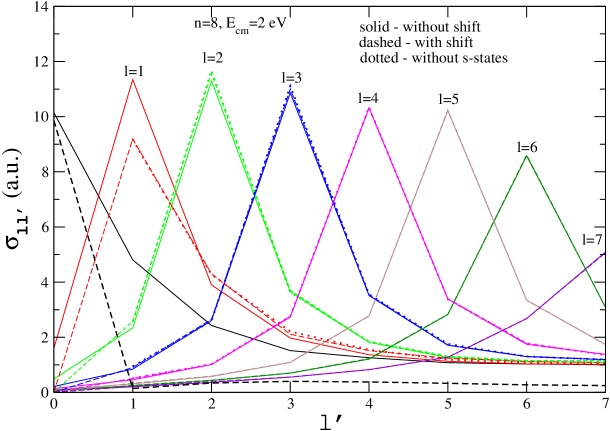
Figure 1: The total cross sections $\sigma_{nl\to nl^{\prime}}$ for the collisions of the $p\bar{p}$ atom in the $n=8$ state with hydrogen atom at $E_{\rm cm}=1.4$ eV. The dashed and dotted lines connect the points corresponding to the calculations both with and without taking into account the $ns$-state energy shifts, respectively. The dotted lines denote the results obtained without including the $ns$-states into the basis set.

The results of the calculations are presented in Figures 1-4. In Fig. 1 we introduced the calculated total cross sections of the $nl\to nl^{\prime}$ transitions for $n=8$ at the kinetic energy $E_{\rm cm}=1.4$ eV both with and without the $ns$ state energy shifts. The following measured world-average value 17 for the spin-averaged shift

$$\epsilon_{1s}=(721\pm 14){\rm eV}$$

was used in the present calculations and the energy shifts of the $ns$ states are defined by $\epsilon_{1s}/n^{3}$.

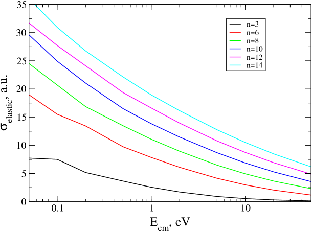
Figure 2: The $l$-averaged cross sections of the elastic scattering for the collisions of the $p\bar{p}$ atom with the hydrogenic atom for the different values of the principal quantum number $n$

Contrary to the $(\pi^{-}p)$-atom, the energy shifts of the $ns$ states in $(\bar{p}p)$-atom are repulsive, hence, the $nl\to ns$ transitions are closed below the corresponding threshold and, besides, according to the present study (e.g., see Fig. 1) the Stark transitions both from the $ns$-states and to the $ns$-state at the same collisional energy are strongly suppressed at the kinetic energies above the threshold. The similar effect is also observed for the elastic $np\to np$ transitions. The other transitions are practically unchangeable at fixed energy. The analog of this effect can be modeled by excluding $ns$-states from the basis states. At energy above a few thresholds the effect is much weaker. Therefore, the strong interaction effect in the antiprotonic hydrogen (the similar effect must be also observed in the kaonic hydrogen atom) results in the essential and important difference of the Stark transition role in the absorption from the $ns$ states in contrast to pionic hydrogen atoms. The influence of the strong interaction shift enhances for the lower states and becomes less pronounced for the highly excited states of the antiprotonic atom.

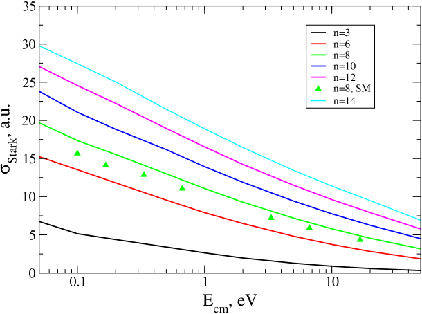
Figure 3: The $l$-averaged cross sections of the Stark transitions for the collisions of the $p\bar{p}$ atom with the hydrogenic one. The results of the calculations 10 in the semiclassical model are shown for $n=8$ with triangles

In Figures 2 and 3 the energy dependence of the $l$-averaged total elastic and Stark cross sections are shown for the different principle quantum number values from $n=3$ up to $n=12$. Since the relative contribution of the $ns$ state in the $l$-averaged cross sections are small, the calculations both with and without the energy shift are practically indistinguishable at the energies above the corresponding threshold. So, in Figs. 2 and 3 the small energy region (below the corresponding threshold) corresponds to the calculations without the energy shift taken into account. In Fig. 3 the $l$-averaged cross section for $n$=8 are compared with the calculations in the framework of the semiclassical model 10 . As a whole a fair agreement is observed, but the semiclassical model results in a different energy dependence especially at low energy collision and gives smaller cross sections than those obtained in the present approach.

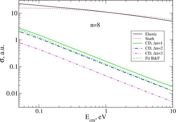
Figure 4: The $l$-averaged cross sections of Coulomb deexcitation with $\Delta n=1,2,3$ for the collisions of the $p\bar{p}$ atom ($n=8$) with the hydrogenic atom. The dashed line shows the fit used in cascade calculations 13 for the transitions with $\Delta n=1$and based on the mass-scaling of the results 11 for the muonic atom. The present calculations of the $l$-averaged elastic and Stark cross sections are shown for comparison

The dependence of the Coulomb deexcitation cross sections on energy obtained in the present study is illustrated in Fig. 4 for $n=8$ and the different values of $\Delta n$ =1, 2 and 3. The special features of these cross sections are the following: the similar energy dependence but sharper than that of the elastic scattering and Stark transitions (see also in Fig. 4); the contribution of the transitions with $\Delta n>1$ is comparable with the one for $\Delta n$ =1 and approximately equal about 50%. The effect of the $ns$ state energy shifts in the $l$-averaged Coulomb deexcitation cross sections are small for the same reason as it was discussed above (due to small statistical weight of the ns-state). In Fig. 4 we also compare our results with those obtained in the semiclassical model (we use the parameterization suggested in [13] which gives a fair description of the Coulomb cross sections from [11]) for the $\Delta n$ =1 transition. The satisfactory agreement is observed, but this agreement is quite occasional and takes no place for other $n$ values. The distribution over the final states $n^{\prime}$ is completely different from the semiclassical results [11] as it was illustrated in Fig. 4. The present calculations predict that $\Delta n>1$ transitions give a substantial contribution to the Coulomb deexcitation of the highly excited antiprotonic hydrogen atom that is in agreement with our previous results for the muonic and pionic hydrogen [14,15] atoms.

IV Conclusion

The unified treatment of the elastic scattering, Stark transitions and Coulomb deexcitation is presented in ab initio quantum-mechanical approach and for the first time the cross sections of these processes have been calculated for the highly excited antiprotonic hydrogen atom. The influence of the energy shifts of the $ns$ states on these processes has been studied. We have found that strong interaction shifts in the antiprotonic hydrogen atom lead to substantial suppression of both the $ns\to nl^{\prime}\neq 0$ and $nl^{\prime}\neq 0\to ns$ transitions. At the same time the cross sections of the elastic scattering and Stark transitions for the the states with $l>2$ are practically unchangeable. The present study is the first step to achieving a reliable theoretical input for realistic kinetics calculations.

We are grateful to Prof. L.Ponomarev for the stimulating interest and support of this investigation.

References

• (1) D. Gotta et al., Newsletter 15, 276 (1999).
• (2) J.F.Crawford et al., Phys.Rev. D 43, 46 (1991).
• (3) M.Leon and H.A.Bethe, Phys.Rev. 127, 636 (1962).
• (4) T.P.Terrado and R.S. Hayano, Phys.Rev. C 55, 73, (1977).
• (5) V.P.Popov and V.N.Pomerantsev, Hyp. Interact. 101/102, 133 (1996).
• (6) V.P.Popov and V.N.Pomerantsev, Hyp. Interact. 119, 133 (1999).
• (7) V.P.Popov and V.N.Pomerantsev, Hyp. Interact. 119, 137 (1999).
• (8) V.V.Gusev, V.P.Popov and V.N.Pomerantsev, Hyp. Interact. 119, 141 (1999).
• (9) T.S.Jensen and V.E.Markushin, PSI-PR-99-32 (1999); nucl-th/0001009.
• (10) T.S.Jensen and V.E.Markushin, Eur.Journ.Phys. D, 19, 165 (2001).
• (11) L.Bracci and G.Fiorentini, Nuovo Cim. 43A, 9 (1978).
• (12) T.S.Jensen and V.E.Markushin, physics/0205076.
• (13) T.S.Jensen and V.E.Markushin, physics/0205077.
• (14) G.Ya. Korenman, V.N. Pomerantsev, and V.P. Popov, JETP Lett. 81, 543 (2005); nucl-th/0501036.
• (15) V.N. Pomerantsev and V.P. Popov, nucl-th/0511026.
• (16) Handbook of mathematical functions, eds. M. Abramowitz and I.A. Stegun, National Bureau of Standards, Applied mathematical series - 55, 1964.
• (17) M.Augsburgeret al., Nucl. Phys. A 658, 149 (1999)