$J/\psi$ Gluonic Dissociation Revisited : III.
Effects of Transverse Hydrodynamic Flow

B. K. Patra1 and V. J. Menon2
1 Dept. of Physics, Indian Institute of Technology, Roorkee 247 667, India

2 Dept. of Physics, Banaras Hindu University, Varanasi 221 005, India


Abstract

In a recent paper [Eur. Phys. J C 44, 567 (2005)] we developed a very general formulation to take into account explicitly the effects of hydrodynamic flow profile on the gluonic breakup of $J/\psi$’s produced in an equilibrating quark-gluon plasma. Here we apply that formulation to the case when the medium is undergoing cylindrically symmetric transverse expansion starting from RHIC or LHC initial conditions. Our algebraic and numerical estimates demonstrate that the transverse expansion causes enhancement of local gluon number density $n_{g}$, affects the $p_{{}_{T}}$-dependence of the average dissociation rate $\langle\tilde{\Gamma}\rangle$ through a partial-wave interference mechanism, and makes the survival probability $S(p_{{}_{T}})$ to change with $p_{{}_{T}}$ very slowly. Compared to the previous case of longitudinal expansion the new graph of $S(p_{{}_{T}})$ is pushed up at LHC, but develops a rich structure at RHIC, due to a competition between the transverse catch-up time and plasma lifetime.


PACS numbers: 12.38M

1 Introduction

It is a well-recognized fact that hydrodynamic expansion can significantly influence the internal dynamics of, and signals coming from, the parton plasma produced in relativistic heavy-ion collisions. The scenario of $J/\psi$ suppression due to gluonic bombardmentΒ [1]-[8] now becomes very nontrivial because of two reasons: i) the flow causes inhomogeneities with respect to the time-space location $x$ and ii) careful Lorentz transformations must be carried out among the rest frames of the fireball, medium, and $\psi$ meson. In a recent paperΒ [8] this nontrivial problem was formally solved by first assuming a general flow velocity profile $\vec{v}(x)$ and thereafter deriving new statistical mechanical expressions for the gluon number density $n_{g}(x)$, average dissociation rate $\langle\tilde{\Gamma}(x)\rangle$, and $\psi$ meson survival probability $S(p_{{}_{T}})$ at transverse momentum $p_{{}_{T}}$ (assuming the meson’s velocity $\vec{v}_{\psi}$ to be along the lateral $X$ direction in the fireball frame).

This general theory was also applied numerically in refΒ [8] to a plasma undergoing pure longitudinal expansion parallel to the collision axis. In such case the kinematics is simple because $\vec{v}\cdot\vec{v}_{\psi}=0$ and also the cooling is knownΒ [9] to occur slowly. When comparison was made with the no flow situationΒ [7] we found that $n_{g}(x)$ was enhanced, a partial wave interference mechanism operated in $\langle\tilde{\Gamma}(x)\rangle$, and the graph of $S(p_{{}_{T}})$ was pushed down/up depending on the LHC/RHIC initial conditions.

The aim of the present paper is to address the following important question: β€œWhat will happen if the general theory of refΒ [8] is applied to the cylindrically symmetric, pure transverse expansion involving tougher kinematics (because vβ†’β‹…vβ†’Οˆβ‰ 0⋅→𝑣subscriptβ†’π‘£πœ“0\vec{v}\cdot\vec{v}_{\psi}\neq 0) as well as higher cooling rateΒ [9]? In Sec.2 below we derive the relevant formulae for statistical observables (viz. $n_{g}$, $\langle\tilde{\Gamma}\rangle$, $S(p_{{}_{T}})$, etc) paying careful attention to the $\psi$ meson trajectory and the so called catch-up time. Next, Sec.3 presents our detailed numerical work along with interpretations concerning $\langle\tilde{\Gamma}\rangle$ and $S(p_{{}_{T}})$. Finally, our main conclusions are summarized in Sec.4.

2 Statistical observables

2.1 Hydrodynamic aspects

We assume local thermal equilibrium and set-up a cylindrical coordinate system in the fireball frame appropriate to central collision. Let $\vec{x}=(r~{}\phi~{}z)$ be a typical spatial point, $x^{\mu}=(t,\vec{x})$ a time-space point, $\vec{v}$ the fluid $3$ velocity, $\gamma={\left(1-v^{2}\right)}^{-1/2}$ the Lorentz factor, $\tau$ the proper time, $u^{\mu}=(\gamma,\gamma\vec{v})$ the $4$ velocity, $P$ the comoving pressure, $\epsilon$ the comoving energy density, $T$ the temperature, and $T^{\mu\nu}=\left(\epsilon+P\right)u^{\mu}u^{\nu}-Pg^{\mu\nu}$ the energy-momentum tensor. Then, the expansion of the system is described by the equation for conservation of energy and momentum of an ideal fluid

$\displaystyle\partial_{\mu}T^{\mu\nu}=0,$ (2.1)

in conjunction with the equation of state for a partially equilibrated plasma of massless particles

$\displaystyle\epsilon=3P=\left[a_{2}\lambda_{{}_{g}}+b_{2}(\lambda_{{}_{q}}+\lambda_{{}_{\bar{q}}})\right]T^{4}$ (2.2)

where $a_{2}=8\pi^{2}/15$, $b_{2}=7\pi^{2}N_{f}/40$, $N_{f}\approx 2.5$ is the number of dynamical quark flavors, $\lambda_{{}_{g}}$ is the gluon fugacity, and $\lambda_{{}_{\bar{q}}}$ ($\lambda_{{}_{q}}$) is the (anti-) quark fugacity. Of course, the gluons (or quarks) obey Bose-Einstein (or Fermi-Dirac) statistics having fugacities $\lambda_{{}_{g}}$ (or $\lambda_{{}_{q}}$). Under transverse expansion the fugacities and temperature evolve with the proper time according to the master rate equationsΒ [10, 11, 12]

$\displaystyle\frac{\gamma}{\lambda_{g}}\partial_{t}\lambda_{g}$ $\displaystyle+$ $\displaystyle\frac{\gamma v_{r}}{\lambda_{g}}\partial_{r}\lambda_{g}+\frac{1}{T^{3}}\partial_{t}(\gamma T^{3})+\frac{v_{r}}{T^{3}}\partial_{r}(\gamma T^{3})$ (2.3)
$\displaystyle+$ $\displaystyle\gamma\partial_{r}v_{r}+\gamma\left(\frac{v_{r}}{r}+\frac{1}{t}\right)$
$\displaystyle=$ $\displaystyle R_{3}(1-\lambda_{g})-2R_{2}\left(1-\frac{\lambda_{q}\lambda_{\bar{q}}}{\lambda_{g}^{2}}\right)\,,$
$\displaystyle\frac{\gamma}{\lambda_{q}}\partial_{t}\lambda_{q}$ $\displaystyle+$ $\displaystyle\frac{\gamma v_{r}}{\lambda_{q}}\partial_{r}\lambda_{q}+\frac{1}{T^{3}}\partial_{t}(\gamma T^{3})+\frac{v_{r}}{T^{3}}\partial_{r}(\gamma T^{3})$ (2.4)
$\displaystyle+$ $\displaystyle\gamma\partial_{r}v_{r}+\gamma\left(\frac{v_{r}}{r}+\frac{1}{t}\right)$
$\displaystyle=$ $\displaystyle R_{2}\frac{a_{1}}{b_{1}}\left(\frac{\lambda_{g}}{\lambda_{q}}-\frac{\lambda_{\bar{q}}}{\lambda_{g}}\right)\,,$

where the symbols are defined by

$\displaystyle R_{2}=0.5n_{g}\langle v\sigma_{gg\longrightarrow q\bar{q}}\rangle,\quad R_{3}=0.5n_{g}\langle v\sigma_{gg\longrightarrow ggq}\rangle$ (2.5)

For our phenomenological purposes it will suffice to assume that, at a general instant $t$ in the fireball frame, the plasma is contained in a uniformly expanding cylinder of radius

$\displaystyle R=R_{i}+\left(t-t_{i}\right)v_{e}$ (2.6)

where $R_{i}$ was the radius at the initial instant $t_{i}$ and the expansion speed $v_{e}$ is a free parameter $(0\leq v_{e}<1)$. In absence of azimuthal rotations the transverse velocity profile of the medium can be parametrized by a linear ansatz

$\displaystyle\vec{v}=v_{e}~{}\vec{r}/R,\qquad 0\leq r\leq R$ (2.7)

Clearly, $|\vec{v}|$ vanishes at the origin but becomes $v_{{}_{e}}$ at the edge. The (chemical) master equations (2.3 - 2.4) are designed to be solved numerically on a computer subject to the RHIC/LHC initial conditions stated in Table 1:

Table 1: Colliding nuclei, collision energy, and initial parameters for the QGP at RHIC(1), LHC(1)Β [13].
Nuclei Energy $\sqrt{s}$ $t_{i}$ $T_{i}$ $\lambda_{{}_{gi}}$ $\lambda_{{}_{qi}}$ $R_{i}$
(GeV/nucleon) (fm/c) (GeV) (fm)
RHIC(1) ${\mbox{Au}}^{197}$ 200 0.7 0.55 0.05 0.008 6.98
LHC(1) ${\mbox{Pb}}^{208}$ 5000 0.5 0.82 0.124 0.02 7.01

The lifetime or freeze-out time $t_{\mbox{life}}$ of the plasma is the instant when the temperature at the edge falls to $T(t_{\mbox{life}})=0.2$ GeV, say.

2.2 Gluon number density

For arbitrary flow profile $\vec{v}$, momentum integrationΒ [8, eq.(11)] over a Bose-Einstein distribution function yields the evolving gluon number density

$\displaystyle n_{g}(x)=\frac{16}{\pi^{2}}~{}\gamma~{}T^{3}\sum_{n=1}^{\infty}\frac{\lambda_{g}^{n}}{n^{3}}$ (2.8)

Since this expression does not depend on the angles of $\vec{v}$ it has the same structure both for the longitudinal and transverse cases. Also, flow enhances the number density compared to the no-flow caseΒ [7]; e.g. at fixed $\lambda_{{}_{g}}$ the enhancement factor $\gamma$ becomes $2.3$ if $|\vec{v}|=0.9~{}c$.

2.3 Average $\psi$ dissociation rate

In the fireball frame (keeping the flow profile still general) we consider a $\psi$ meson of mass $m_{\psi}$, four momentum $p^{\mu}_{\psi}$, three velocity $\vec{v}_{\psi}=\vec{p}_{\psi}/p^{0}_{\psi}$, and Lorentz factor $\gamma_{\psi}=p^{0}_{\psi}/m_{\psi}$. If $w^{\mu}$ is the plasma $4$ velocity measured in the rest frame of $\psi$ then we can define the useful kinematic symbolsΒ [8, eq.(30)]

$\displaystyle F=\vec{v}\cdot\hat{v}_{\psi},\qquad Y=\gamma_{\psi}|\vec{v}_{\psi}|-\left(\gamma_{\psi}-1\right)F$
$\displaystyle w^{0}=\gamma\gamma_{\psi}\left(1-F|\vec{v}_{\psi}|\right),\qquad\vec{w}=\gamma\left(\vec{v}-Y\hat{v}_{\psi}\right)$
$\displaystyle\cos\theta_{\psi w}=\hat{w}\cdot\hat{v}_{\psi}=\gamma\left(F-Y\right)/|\vec{w}|$ (2.9)

where the caps stand for unit vectors. Now, let $q^{\mu}$ be the gluon $4$ momentum seen in the $\psi$ meson rest frame, $\epsilon_{\psi}$ the $c\bar{c}$ binding energy, $Q^{0}=q^{0}/\epsilon_{\psi}$ a dimensionless variable, and $\sigma_{{}_{\rm{Rest}}}(Q^{0})\propto{\left(Q^{0}-1\right)}^{3/2}/{Q^{0}}^{5}$ the $g-\psi$ breakup cross section according to QCDΒ [14]. Then, the mean dissociation rate due to hard thermal gluonsΒ [8, eq.(32)] is given by

$\displaystyle\langle\tilde{\Gamma}(x)\rangle$ $\displaystyle=$ $\displaystyle\frac{8\epsilon_{\psi}^{3}\gamma_{\psi}}{\pi^{2}}\sum_{n=1}^{\infty}\lambda_{g}^{n}\int_{1}^{\infty}dQ^{0}{Q^{0}}^{2}\sigma_{\rm{Rest}}(Q^{0})e^{-C_{n}Q^{0}}$ (2.10)
$\displaystyle\times$ $\displaystyle\left[\frac{}{}I_{0}(\rho_{n})+I_{1}(\rho_{n})|\vec{v}_{\psi}|\cos\theta_{\psi w}\frac{}{}\right]$

where we have used the abbreviations

$\displaystyle C_{n}=n\epsilon_{\psi}w^{0}/T,\qquad D_{n}=n\epsilon_{\psi}|\vec{w}|/T$
$\displaystyle\rho_{n}=D_{n}Q^{0},\qquad I_{0}(\rho_{n})=\sinh(\rho_{n})/\rho_{n}$
$\displaystyle I_{1}(\rho_{n})=\cosh(\rho_{n})/\rho_{n}-\sinh(\rho_{n})/\rho_{n}^{2}$ (2.11)

Equation (2.10) demonstrates how $\langle\tilde{\Gamma}(x)\rangle$ depends on the hydrodynamic flow through $w^{\mu}$ as well as the angle $\theta_{\psi w}$. Retaining only the $n=1$ term and picking-up the dominant peak contribution from $Q^{0}_{p}=10/7$ we arrive at the useful approximation

$\displaystyle{\langle\tilde{\Gamma}(x)\rangle}\propto\lambda_{g}\gamma_{\psi}H$
$\displaystyle H\equiv e^{-C_{1}Q^{0}_{p}}\left[\frac{}{}I_{0}(D_{1}Q^{0}_{p})+I_{1}(D_{1}Q^{0}_{p})\mid\vec{v}_{\psi}\mid\cos\theta_{\psi w}\frac{}{}\right]$ (2.12)

in which a partial wave interference mechanism operates due to the anisotropic $\cos\theta_{\psi\omega}$ factor. Numerical consequences of (2.10) relevant to transverse flow will be discussed later in Sec.3.1.

2.4 $J/\psi$ Survival probability

In this section we shall consider pure transverse flow parametrized by (2.7) and the $\psi$ meson moving in the lateral $X$ direction with velocity $\vec{v}_{\psi}=(v_{{}_{T}}~{}0~{}0)$ appropriate to the mid-rapidity region in the fireball frame. Suppressing the $z$ coordinate the production configuration of $\psi$ meson is called $\left(t_{I},\vec{r}^{I}_{\psi}\right)\equiv\left(t_{I},r^{I}_{\psi},\phi^{I}_{\psi}\right)$ and the general trajectory after time duration $\Delta$ is termed $\left(t,\vec{r}_{\psi}\right)\equiv\left(t,r_{\psi},\phi^{I}_{\psi}\right)$ such that

$\displaystyle t_{I}=t_{i}+\gamma_{\psi}\tau_{{}_{F}},\qquad\Delta=t-t_{I}$
$\displaystyle\vec{r}_{\psi}=\vec{r}^{I}_{\psi}+\vec{v}_{\psi}\Delta$ (2.13)

where $\tau_{F}\approx 0.89~{}{\mbox{fm/c}}$ is the proper formation timeΒ [15] of the $c\bar{c}$ bound state. This transverse trajectory will hit the edge $R\equiv R_{I}+v_{e}~{}\Delta$ of the radially expanding cylinder (cf.(2.6)) at the catch-up instant $t^{\ast}$ after duration $\Delta^{{}^{\ast}}$ such that

$\displaystyle{\mid R_{I}+v_{e}\Delta^{\ast}\mid}^{2}={\mid\vec{r}^{I}_{\psi}+\vec{v}_{\psi}\Delta^{\ast}\mid}^{2}$
$\displaystyle{\mbox{so}}\quad\alpha{\Delta^{\ast}}^{2}+2\beta\Delta^{\ast}-\mu=0$
$\displaystyle{\mbox{with}}\quad\alpha=v_{\psi}^{2}-v_{e}^{2},\qquad\mu=R_{I}^{2}-{r_{\psi}^{I}}^{2}$
$\displaystyle\beta=r_{\psi}^{I}v_{\psi}\cos\phi_{\psi}^{I}-R_{{}_{I}}v_{e}$ (2.14)

If the quadratic in $\Delta^{\ast}$ has real roots we pick up that which is positive and smaller; but if both roots are imaginary then catch-up cannot occur. The time interval of physical interest becomes

$\displaystyle t_{I}\leq t\leq t_{II},\qquad t_{II}={\mbox{min}}\left(t_{I}+\Delta^{\ast},~{}t_{\mbox{life}}\right)$ (2.15)

This formula is quite different from that derived in the case of longitudinal flowΒ [8, eq.(48)]. As the time $t$ progresses the dissociation rate (2.10) must be evaluated on the $\psi$ meson trajectory itself, implying that we have to set at a general instant

$\displaystyle\vec{r}=\vec{r}_{\psi},\qquad\vec{v}=v_{e}~{}\vec{r}_{\psi}/R$
$\displaystyle F\equiv\vec{v}\cdot\hat{v}_{\psi}=\left(\frac{v_{e}}{R}\right)\left(r_{\psi}^{I}\cos\phi_{\psi}^{I}+v_{\psi}\Delta\right)$ (2.16)

in the kinematic relations (2.9). Clearly, the notation $\langle\tilde{\Gamma}\rangle$ of (2.10) becomes equivalent to

$\displaystyle\langle\tilde{\Gamma}[t]\rangle\equiv\langle\tilde{\Gamma}(t,p_{{}_{T}},r_{\psi}^{I},\phi^{I}_{\psi})\rangle$ (2.17)

depending parametrically on the production configuration $r^{I}_{\psi}$, $\phi^{I}_{\psi}$. Then, by using the radioactive decay law without recombination and averaging over the cross sectional area $A_{I}=\pi R_{I}^{2}$ (at the production instant) we arrive at the desired survival probability

$\displaystyle S(p_{T})=\int_{A_{I}}d^{2}r_{\psi}^{I}(R_{I}^{2}-{r_{\psi}^{I}}^{2})e^{-W}/\int_{A_{I}}d^{2}r_{\psi}^{I}(R_{I}^{2}-{r_{\psi}^{I}}^{2})$
$\displaystyle W=\int_{t_{{}_{I}}}^{t_{{}_{II}}}dt~{}~{}\tilde{\Gamma}[t],\qquad d^{2}r_{\psi}^{I}=dr_{\psi}^{I}~{}r_{\psi}^{I}~{}d\phi_{\psi}^{I}$ (2.18)

Here no information is needed about the length $L_{I}$ of the cylindrical plasma in contrast to the case of longitudinal flowΒ [8, eq.(52)] where the averaging had to be done over the volume $V_{I}=\pi R_{I}^{2}L_{I}$.

3 Numerical results

3.1 Curves of dissociation rate

The exact formula (2.10) of $\langle\tilde{\Gamma}\rangle$ is a very complicated function of $t$ as well as several kinematic parameters defined jointly by (2.9, 2.11, 2.16) but a feeling for its behaviour can be obtained in the extreme nonrelativistic $\left(|\vec{v}|/c\rightarrow 0\right)$ and ultrarelativistic $\left(|\vec{v}|/c\rightarrow 1\right)$ limits. For simplicity, suppose at the instant $t_{I}$ a special $\psi$ was formed almost at the edge $R_{I}$ of the cylinder with $\phi^{I}_{\psi}$ being the angle between the $\psi$ position vector and velocity vector. Then the kinematic relations (2.16, 2.9) yield

$\displaystyle\vec{v}=v_{{}_{e}}\hat{r}^{I}_{\psi}=\pm v_{{}_{e}}\hat{v}_{\psi},\quad F=v_{{}_{e}}\cos\phi^{I}_{\psi}=\pm v_{{}_{e}}$
$\displaystyle\vec{w}=\gamma\left(\vec{v}-Y\hat{v}_{\psi}\right)=\gamma_{e}\left(\pm v_{{}_{e}}-Y\right)\hat{v}_{\psi}$ (3.1)

where the $+$, $-$ signs correspond to $\cos\phi^{I}_{\psi}=\pm 1$, i.e., to $\phi^{I}_{\psi}=0,\pi$, respectively. Thus we have the parallel or anti-parallel property

$\displaystyle\vec{w}\parallel\hat{v}_{\psi},\quad\cos\phi_{\psi w}=+1~{}{\mbox{if}}~{}\phi^{I}_{\psi}=0~{}\&~{}Y<v_{{}_{e}}$
$\displaystyle\vec{w}\parallel-\hat{v}_{\psi},\quad\cos\phi_{\psi w}=-1~{}{\mbox{if}}~{}\phi^{\pm}_{\psi}=\pi~{}{\mbox{or}}~{}Y>v_{{}_{e}}$ (3.2)

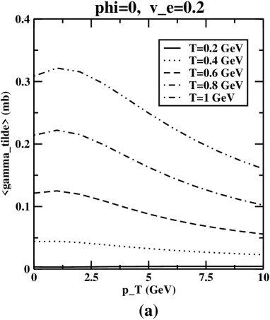
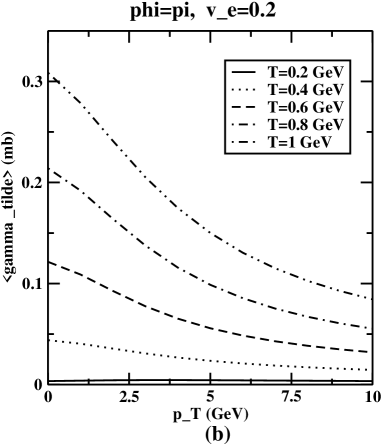
Figures 1 - 4 depict the corresponding exact curves of $\langle\tilde{\Gamma}\rangle$ computed from (2.10) based on the LHC initial conditions of Table 1. We now proceed

Β Β Β Β Β Β Β Β Β Refer to caption Β Β Β Β Β Β Β Β Β Refer to caption

Figure 1: The variation of the modified rate $\langle\tilde{\Gamma}\rangle$ as a function of temperature at different transverse momenta for the transverse flow velocity $v=0.2~{}c$ for (a) $\phi^{I}_{\psi}=0$ and (b) $\phi^{I}_{\psi}=\pi$, respectively.

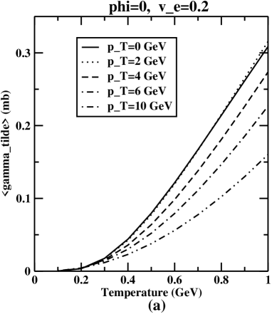
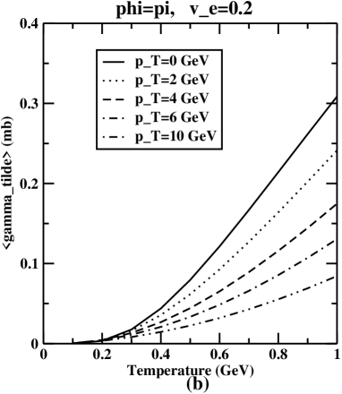
to interpret these graphs using the approximate estimate (2.12).

Interpretation: i) At fixed $(p_{{}_{T}},\phi^{I}_{\psi},v_{{}_{e}})$ the steady increase of $\langle\tilde{\Gamma}\rangle$ with $T$ in Figs.1 - 2 is caused by the growing $\exp\{-(C_{1}\mp D_{1})Q^{0}_{p}\}$ factors occurring in the estimate (2.12).
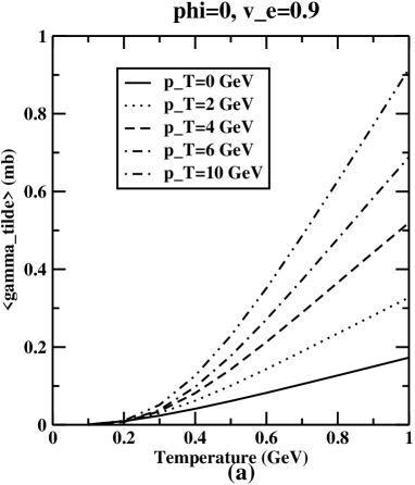
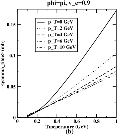
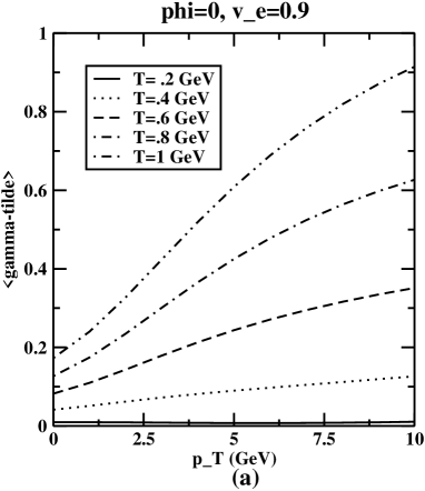
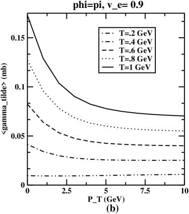
Β Β Β Β Β Β Β Β Β Refer to caption Β Β Β Β Β Β Β Β Β Refer to caption

Figure 2: The variation of the modified rate $\langle\tilde{\Gamma}\rangle$ as a function of temperature at different transverse momenta for the transverse flow velocity $v=0.9~{}c$ for (a) $\phi^{I}_{\psi}=0$ and (b) $\phi^{I}_{\psi}=\pi$, respectively.

Β Β Β Β Β Β Β Β Β Refer to caption Β Β Β Β Β Β Β Β Β Refer to caption

Figure 3: The variation of the modified rate $\langle\tilde{\Gamma}\rangle$ as a function of transverse momentum for different values of temperatures for a transverse flow velocity $v=0.2~{}c$ for (a) $\phi^{I}_{\psi}=0$ and (b) $\phi^{I}_{\psi}=\pi$, respectively.

Β Β Β Β Β Β Β Β Β Refer to caption Β Β Β Β Β Β Β Β Β Refer to caption

Figure 4: The variation of the modified rate $\langle\tilde{\Gamma}\rangle$ as a function of transverse momentum at different values of temperatures for a transverse flow velocity $v=0.9~{}c$ for (a) $\phi^{I}_{\psi}=0$ and (b) $\phi^{I}_{\psi}=\pi$, respectively.

ii) At fixed value of $(T,\phi^{I}_{\psi},v_{{}_{e}}=0.2)$ corresponding to nonrelativistic flow the variation of $\langle\tilde{\Gamma}\rangle$ with $p_{{}_{T}}$ in Figs.3a,b is more intricate. At $\phi^{I}_{\psi}=0$ in Fig.3a there is a broad enhancement of $\langle\tilde{\Gamma}\rangle$ for low $p_{{}_{T}}\leq 1$ GeV; this is because, firstly low speeds of the $\psi$ and plasma can compete, and secondly constructive interference occurs between $I_{0}$ and $I_{1}$ in the estimate (2.12) for $\cos\theta_{\psi w}=+1$ (cf.(3.2)). On the other hand, at $\phi^{I}_{\psi}=\pi$ in Fig.3b our $\langle\tilde{\Gamma}\rangle$ decreases monotonically with $p_{{}_{T}}$ throughout; this is due to the fact that, since $\cos\theta_{\psi w}=-1$ now (cf.(3.2)), the interference between $I_{0}$ and $I_{1}$ becomes destructive. iii) At fixed values of $(T,\phi^{I}_{\psi},v_{{}_{e}}=0.9)$ corresponding to ultrarelativistic flow similar trends with respect to $p_{{}_{T}}$ are again explained in Figs.4a, b except for the fact that the steady rise of $\langle\tilde{\Gamma}\rangle$ with $p_{{}_{T}}$ in Fig.4a is caused mainly by the $\gamma_{\psi}$ coefficient present in the estimate (2.12).

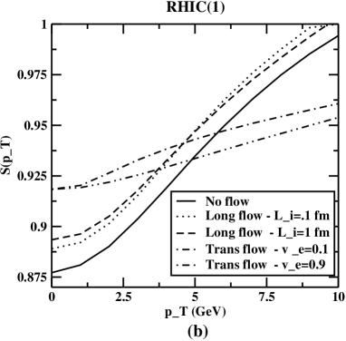
3.2 Curves of survival probability

For a chosen creation configuration of the $\psi$ meson the function $W$ was first computed from (2.18) and then $S(p_{{}_{T}})$ was numerically evaluated. Figures 5a and 5b show the dependence of $S(p_{{}_{T}})$ on $p_{{}_{T}}$ corresponding to the LHC and RHIC initial conditions, respectively (for two choices of the transverse expansion speed $v_{{}_{e}}$). For the sake of direct comparison, we also include our earlier results based on no flow Β [7, eq.(25)] and longitudinal expansionΒ [8, eq.(52)] (starting from two possible lengths $L_{i}$ of the initial cylinder). We now turn to a physical discussion of these graphs.

Β Β Β Β Β Β Β Β Β Refer to caption Β Β Β Β Β Β Β Β Β Refer to caption

Figure 5: The survival probability of $J/\psi$ in an equilibrating parton plasma at (a) LHC(1) and (b) RHIC(1) energies with initial conditions given in Table 1. The solid curve $S_{0}(p_{{}_{T}})$ is the result ofΒ [7], i.e., in the absence of flow while the dotted and dashed curves represent the $S_{\parallel}(p_{{}_{T}})$ when the plasma is undergoing longitudinal expansion with the initial values of the length of the cylinder $L_{i}=0.1$ fm and $1$ fm, respectivelyΒ [8]. The dot-dashed and and double dot-dashed curves depict the $S_{\perp}(p_{{}_{T}})$ when the system is undergoing transverse expansion with the expansion speed $v_{{}_{e}}=0.1$ and $0.9$, respectively.

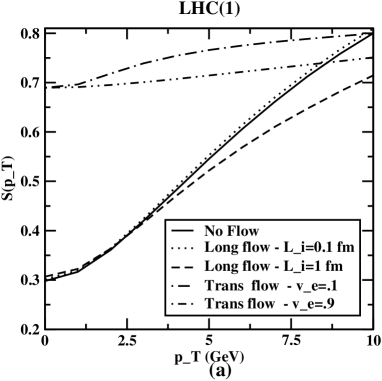
Interpretation: In every scenario of gluonic dissociation the function $W=\int_{t_{I}}^{t_{II}}dt~{}\langle\tilde{\Gamma}\rangle$ depends on $p_{{}_{T}}$ via the integrand $\langle\tilde{\Gamma}\rangle$ as well as the limits $(t_{I},t_{II})$. Three interesting cases may now be distinguished:

No flow caseΒ [7]: Here cooling of the plasma is simulated through the master rate equations but the existence of the explicit flow profile is ignored. Then $\langle\tilde{\Gamma}\rangle$ decreases monotonically with $p_{{}_{T}}$ because of a destructive interference between the $I_{0}$ and $I_{1}$ terms. Also, the time-span $t_{{}_{II}}-t_{{}_{I}}$ is shortened as the speed of the $\psi$ meson increases. Consequently, the survival probability called $S_{0}(p_{{}_{T}})$ grows steadily with $p_{{}_{T}}$ as shown by the solid lines in Figs.5a,b.

Longitudinal expansion case: Here an extra parameter appears namely the length $L_{i}$ of the initial cylinder. For nonrelativistic flow emanating from short length $L_{i}=0.1$ fm the $\langle\tilde{\Gamma}\rangle$ values are somewhat reduced compared to the no flow case (due to $I_{0}$, $I_{1}$ destructive interference) though the time span $t_{{}_{II}}-t_{{}_{I}}$ remains unaltered, so that the survival probability called $S_{\parallel}(p_{{}_{T}})$ is pushed slightly upwards in Figs.5a,b. But for relativistic flow emanating from longer length $L_{i}=1$ fm the shifts of the $S_{\parallel}(p_{{}_{T}})$ curve occurs in mutually opposite directions at LHC and RHIC (due to the different initial temperatures generated therein).

Transverse expansion case: Here the extra parameter involved is the transverse expansion speed $v_{{}_{e}}$ which together with $\phi^{I}_{\psi}$ and $T$ control the $p_{{}_{T}}$-dependence of the function $W$. For $\phi^{I}_{\psi}=0$ the $\langle\tilde{\Gamma}\rangle$ values in Figs.3a, 4a exhibit enhancement/rising trend on the lower $p_{{}_{T}}$ side; such $\psi$ mesons contribute sizably to $W$ but little to $e^{-W}$. On the othe hand, all curves of $\langle\tilde{\Gamma}\rangle$ in Figs.3 - 4 flatten-off to nearly constant values on the higher $p_{{}_{T}}$ side; such $\psi$ mesons contribute substantially to $e^{-W}$ especially for low temperatures. Therefore, the transverse survival probability $S_{\perp}(p_{{}_{T}})$ becomes nearly $p_{{}_{T}}$-independent (or very slowly varying) in Figs.5a, 5b in sharp contrast to the longitudinal case. For explaining the magnitude of the ratio $S_{\perp}(p_{{}_{T}})/S_{\parallel}(p_{{}_{T}})$ we consider the temporal scenario dealing with the limits of the integration.

Temporal scenario: It is known that transverse expansion of a quark-gluon plasma produces cooling at a faster rate compared to longitudinal expansion so that the inequality $t^{\perp}_{\mbox{life}}<t^{\parallel}_{\mbox{life}}$ holds on the corresponding lifetimes. At LHC the transverse cooling is so fast that, for most $\psi$ mesons of kinematic interest we have $t_{II}=t_{\mbox{life}}^{\perp}$ in the definition (2.15). The time-span $t_{{}_{II}}-t_{{}_{I}}$ is, therefore, much smaller compared to the longitudinal case implying thet $S_{\perp}(p_{{}_{T}})>S_{\parallel}(p_{{}_{T}})$ in Fig.5a. Clearly this property at LHC is devoid of any rich structure.

However, at RHIC let us divide the $\psi$ meson kinematic region into two parts. For slower mesons having $p_{{}_{T}}<5$ GeV the catch-up time $t_{I}+\Delta^{\ast}$ in (2.15) exceeds the lifetime so that $t_{II}=t_{\mbox{life}}^{\perp}$ again, i.e., $S_{\perp}(p_{{}_{T}})>S_{\parallel}(p_{{}_{T}})$ in Fig.5b for $p_{{}_{T}}<5$ GeV. Next, for faster mesons having $p_{{}_{T}}>5$ GeV the reverse inequalities hold making $S_{\perp}(p_{{}_{T}})<S_{\parallel}(p_{{}_{T}})$ in Fig.5b. Clearly, the rich structure in $S_{\perp}(p_{{}_{T}})$ at RHIC arises from a mutual competition between the catch-up time and lifetime.

4 Conclusions

a) In this work we have applied our general formulationΒ [8] of hydrodynamic expansion to study the effect of explicit transverse flow profile on the gluonic break up of $J/\psi$’s created in an equilibrating QGP. The formalism in Sec.2 and numerical results of Sec.3 are new and original.

b) Equation (2.8) shows that, at specified fugacity $\lambda_{{}_{g}}$, the effect of transverse flow is to increase the gluon number density $n_{g}$. This was also the case with longitudinal flow.

c) Our expressions (2.10, 2.12) of the mean dissociation rate $\langle\tilde{\Gamma}\rangle$ involves hyperbolic functions as well as partial wave interference mechanism (controlled by the anisotropic $\cos\theta_{\psi w}$ factor). In addition, knowledge about a nontrivial kinematic function $F$ (cf.(2.16)) is needed for interpreting the variation of $\langle\tilde{\Gamma}\rangle$ with $T$, $p_{{}_{T}}$, $\phi^{I}_{\psi}$, $v_{{}_{e}}$ in Figs.1 - 4. In contrast, for longitudinal flow the treatment of $\langle\tilde{\Gamma}\rangle$ was easier because $F=0$ there.

d) There are several features of contrast between the transverse and longitudinal survival probabilities denoted by $S_{\perp}(p_{{}_{T}})$ and $S_{\parallel}(p_{{}_{T}})$, respectively. Due to the geometry of production configuration our $S_{\perp}(p_{{}_{T}})$ contains a double integral (2.18) whereas $S_{\parallel}(p_{{}_{T}})$ contains a triple integral. Next, due to the flattening-off trend of $\langle\tilde{\Gamma}\rangle$ with increasing $p_{{}_{T}}$ our $S_{\perp}(p_{{}_{T}})$ becomes roughly $p_{{}_{T}}$-independent (or slowly varying) in Figs.5a, 5b whereas $S_{\parallel}(p_{{}_{T}})$ rises rapidly. Finally, the quick cooling rate at LHC makes $S_{\perp}(p_{{}_{T}})>S_{\parallel}(p_{{}_{T}})$ at all $p_{{}_{T}}$ of interest in Fig.5a whereas a competition between the catch-up time and lifetime generates richer structure at RHIC in Fig.5b.

e) We conclude with the observation that the field of $J/\psi$ suppression due to gluonic break up continues to be a research area of great challenge. In a future communication we plan to study the effect of asymmetric flow profile arising from noncentral collision of heavy ions at finite impact parameter $\vec{b}$.

ACKNOWLEDGEMENTS

VJM thanks the UGC, Government of India, New Delhi for financial support. We are also thankful to Dr. Dinesh Kumar Srivastava for discussing in the early stages of this work.

References

  • [1] Helmut Satz, Rept.Prog.Phys. 63, 1511 (2000).
  • [2] D. Kharzeev and H. Satz, Phys. Lett.B 334, 155 (1994).
  • [3] D. Kharzeev and H. Satz, Phys. Lett. B366, 316 (1996).
  • [4] B. K. Patra and V. J. Menon, Nucl. Phys.A708, 353 (2002).
  • [5] Xiao-Ming Xu, D. Kharzeev, H. Satz, and Xin-Nian Wang, Phys. Rev.C53, 3051 (1996).
  • [6] B. K. Patra, D. K. Srivastava, Phys. Lett.B505, 113 (2001).
  • [7] B. K. Patra and V. J. Menon, $J/\psi$-gluonic dissociation revisited:I. Fugacity, flux, and formation time effects, Eur. Phys.J.C 37, 115 (2004).
  • [8] B. K. Patra and V. J. Menon, $J/\psi$ gluonic dissociation revisited:II. Hydrodynamic Expansion Effects, Eur. Phys. J.C44, 567 (2005).
  • [9] D. Pal, B. K. Patra, and D. K. Srivastava, Eur. Phys. J. C 17, 179 (2000).
  • [10] T. S. Biro, E. van Doorn, M. H. Thoma, B. MΓΌller, and X.-N. Wang, Phys. Rev.C48, 1275 (1993).
  • [11] D. K. Srivastava, M.G. Mustafa, and B. MΓΌller, Phys. Rev. C 56, 1064 (1997); Phys. Lett. B 396, 45 (1997).
  • [12] B. K. Patra, J. Alam, P. Roy, S. Sarkar, and B. Sinha, Nucl. Phys. A 709, 440 (2002).
  • [13] X.-N Wang and M. Gyulassy, Phys. Rev.D44, 3501 (1991).
  • [14] M. E. Peskin, Nucl. Phys.B156, 365 (1979); G. Bhanot and M. E. Peskin, Nucl. Phys.B156, 391 (1979).
  • [15] F. Karsch, H. Satz, Z. Phys.C51, 209 (1991); F. Karsch, M.T. Mehr, and H. Satz, Z. Phys.C37, 617 (1988).