Back-to-back Correlations for Finite Expanding Fireballs

Abstract

Back-to-Back Correlations of particle-antiparticle pairs are related to the in-medium mass-modification and squeezing of the quanta involved. They are predicted to appear when hot and dense hadronic matter is formed in high energy nucleus-nucleus collisions. The survival and magnitude of the Back-to-Back Correlations of boson-antiboson pairs generated by in-medium mass modifications are studied here in the case of a thermalized, finite-sized, spherically symmetric expanding medium. We show that the BBC signal indeed survives the finite-time emission, as well as the expansion and flow effects, with sufficient intensity to be observed at RHIC.

I Introduction

Recently, it has been shown ac ; acg that large back-to-back correlations (BBC) of particle-antiparticle pairs of bosonic particles might appear in high energy nucleus-nucleus collisions as a consequence of in-medium mass modification of the bosons. Detailed calculations indicate that the BBC signal appears for values of transverse momenta below 1-2 GeV/c. More recently, it was shown fbbc that BBC of similar strength might appear for fermionic particles as well. The main physical ingredient used in the evaluation of the effects of in-medium modified masses on two particle correlation functions is a quantum-mechanical correlation induced by a nonzero overlap between in-medium and free states. The induced quantum mechanical correlation can be represented in terms of two-mode squeezed states of the asymptotic, observable states and is implemented through a Bogoliubov-Valatin transformation.

The possibility of measuring a significant BBC signal in heavy-ion collisions opens new interesting possibilities for accessing the properties of the matter formed in such collisions. The BBC signal is linked to in-medium mass modifications of hadrons in the hot and dense environment the detected particles experience before freezing out and in this sense BBC measurements provide independent pieces of information on medium modifications from the ones obtained from dilepton yields and spectra. However, there are several additional physical effects that interfere with mass modifications of the detected particles in the interpretation of the BBC signal.

All studies in Refs. ac , acg and fbbc were restricted to infinite, static media. For testing the robustness of the effect, we generalize the previous studies to a more realistic situation of mass modification in a finite-sized, expanding thermalized medium. In this first investigation of such effects, we use a simple hydrodynamical model for the expansion and simple three-dimensional Gaussian profile for the size of the system. Although simple, the model is rich enough to indicate the influence of the expansion and finite-size effect on BBC.

In the next section we review the basic ingredients of the model and in Section III we generalize the model to include expansion effects. Numerical results are presented in Section IV and Section V presents our Conclusions and Future Perspectives.

II Review of The Model - Infinite Homogeneous Medium

In the present paper we concentrate on bosonic BBC and restrict the discussion to cases where the boson is its own antiparticle – like the $\phi$ meson. We are interested in the two-particle correlation function

$$C_{2}({{\mathbf{k}}}_{1},{{\mathbf{k}}}_{2})=\frac{N_{2}({\mathbf{k}}_{1},{\mathbf{k}}_{2})}{N_{1}({\mathbf{k}}_{1})\,N_{1}({\mathbf{k}}_{2})},$$ (1)

where $N_{1}({\mathbf{k}}_{i})$ and $N_{2}({\mathbf{k}}_{1},{\mathbf{k}}_{2})$ are, respectively, the invariant single-particle and two-particle momentum distributions

$$N_{1}({\mathbf{k}}_{1}) = \omega_{{\mathbf{k}}_{1}}\frac{d^{3}N}{d{\mathbf{k}}_{1}}=\omega_{{\mathbf{k}}_{1}}\,\langle a^{\dagger}_{{\mathbf{k}}_{1}}a_{{\mathbf{k}}_{1}}\rangle,$$ (2)

$$N_{2}({\mathbf{k}}_{1},{\mathbf{k}}_{2}) = \omega_{{\mathbf{k}}_{1}}\omega_{{\mathbf{k}}_{2}}\,\langle a^{\dagger}_{{\mathbf{k}}_{1}}a^{\dagger}_{{\mathbf{k}}_{2}}a_{{\mathbf{k}}_{2}}a_{{\mathbf{k}}_{1}}\rangle$$ (3)

$$= \omega_{{\mathbf{k}}_{1}}\omega_{{\mathbf{k}}_{2}}\,\Bigl{[}\langle a^{\dagger}_{{\mathbf{k}}_{1}}a_{{\mathbf{k}}_{1}}\rangle\langle a^{\dagger}_{{\mathbf{k}}_{2}}a_{{\mathbf{k}}_{2}}\rangle+\langle a^{\dagger}_{{\mathbf{k}}_{1}}a_{{\mathbf{k}}_{2}}\rangle\langle a^{\dagger}_{{\mathbf{k}}_{2}}a_{{\mathbf{k}}_{1}}\rangle+\langle a^{\dagger}_{{\mathbf{k}}_{1}}a^{\dagger}_{{\mathbf{k}}_{2}}\rangle\langle a_{{\mathbf{k}}_{2}}a_{{\mathbf{k}}_{1}}\rangle\Bigr{]},$$

where $a^{\dagger}_{\mathbf{k}}$ and $a_{\mathbf{k}}$ are free-particle creation and annihilation operators of scalar quanta, and the angular brackets mean thermal averages. The factorization of the expectation value of four operators into products of expectation values of two operators in Eq.(3) has been derived as a generalization of Wick’s theorem for locally equilibrated (chaotic) systems in Refs.sm ; gykw ; surp . Introducing the chaotic and squeezed amplitudes as

$$G_{c}({{\mathbf{k}}_{1}},{{\mathbf{k}}_{2}}) = \sqrt{\omega_{{\mathbf{k}}_{1}}\omega_{{\mathbf{k}}_{2}}}\;\langle a^{\dagger}_{{\mathbf{k}}_{1}}a_{{\mathbf{k}}_{2}}\rangle,$$ (4)

$$G_{s}({{\mathbf{k}}_{1}},{{\mathbf{k}}_{2}}) = \sqrt{\omega_{{\mathbf{k}}_{1}}\omega_{{\mathbf{k}}_{2}}}\;\langle a_{{\mathbf{k}}_{1}}a_{{\mathbf{k}}_{2}}\rangle,$$ (5)

the two-particle correlation function can be written as

$$C_{2}({{\mathbf{k}}_{1}},{{\mathbf{k}}_{2}})=1+\frac{|G_{c}({{\mathbf{k}}_{1}},{{\mathbf{k}}_{2}})|^{2}}{G_{c}({{\mathbf{k}}_{1}},{{\mathbf{k}}_{1}})G_{c}({{\mathbf{k}}_{2}},{{\mathbf{k}}_{2}})}+\frac{|G_{s}({{\mathbf{k}}_{1}},{{\mathbf{k}}_{2}})|^{2}}{G_{c}({{\mathbf{k}}_{1}},{{\mathbf{k}}_{1}})G_{c}({{\mathbf{k}}_{2}},{{\mathbf{k}}_{2}})}.$$ (6)

The $G_{c}(1,2)$ is the usual Hanbury-Brown-Twiss (HBT) amplitude and $G_{s}(1,2)$ is BBC amplitude.

The thermal average of an operator $\hat{O}$, $\langle\hat{O}\rangle={\rm Tr}(\hat{\rho}\,\hat{O})$, is calculated with a density matrix $\hat{\rho}$ corresponding to medium-modified, thermalized quanta. The crucial point is that the in-medium thermalized quanta are not the ones detected. The detected quanta have energy-momentum $k^{\mu}=(\omega_{\mathbf{k}},{\mathbf{k}})$, $\omega_{{\mathbf{k}}}^{2}={\mathbf{k}}^{2}+m^{2}$ and are described by the creation and annihilation operators $a^{\dagger}_{\mathbf{k}}$ and $a_{\mathbf{k}}$. However, if we denote by $b^{\dagger}_{\mathbf{k}}$ and $b_{\mathbf{k}}$ the creation and annihilation operators of in-medium, thermalized quanta with $k^{*\mu}=(\Omega_{\mathbf{k}},{\mathbf{k}})$, $\Omega^{2}_{\mathbf{k}}={\mathbf{k}}^{2}+m^{2}_{*}(|{\mathbf{k}}|)$, we can relate the $(a^{\dagger}_{\mathbf{k}},a_{\mathbf{k}})$ to $(b^{\dagger}_{\mathbf{k}},b_{\mathbf{k}})$ through a Bogoliubov-Valatin (BV) transformation. Specifically, the annihilation operator $a_{{\mathbf{k}}_{1}}$ for the asymptotic quanta with momentum ${\mathbf{k}}_{1}$ is related to the in-medium operators $b_{{\mathbf{k}}_{1}}$ and $b^{\dagger}_{{\mathbf{k}}_{1}}$ as ac :

$$a_{{\mathbf{k}}_{1}}=c_{{\mathbf{k}}_{1}}\,b_{{\mathbf{k}}_{1}}+s^{*}_{-{\mathbf{k}}_{1}}\,b^{\dagger}_{-{\mathbf{k}}_{1}}\equiv C_{1}+S_{-1}^{\dagger},$$ (7)

where we have introduced the notation $C_{1}=c_{{\mathbf{k}}_{1}}\,b_{{\mathbf{k}}_{1}}$ and $S_{-1}=s^{*}_{-{\mathbf{k}}_{1}}\,b^{\dagger}_{-{\mathbf{k}}_{1}}$ to simplify later notation, and

$$c_{{\mathbf{k}}}=\cosh[f_{{\mathbf{k}}}],\hskip 14.22636pts_{{\mathbf{k}}}=\sinh[f_{{\mathbf{k}}}],\hskip 14.22636ptf_{{\mathbf{k}}}=\frac{1}{2}\log\left(\frac{\omega_{{\mathbf{k}}}}{\Omega_{{\mathbf{k}}}}\right).$$ (8)

The BV transformation for the creation operator $a^{\dagger}_{{\mathbf{k}}_{1}}$ is obtained from Eq. (7) by Hermitean conjugation. As is well known, the Bogoliubov transformation is equivalent to a squeezing operation, and this motivates calling $f_{\mathbf{k}}$ the mode-dependent squeezing parameter. In this way, it is the squeezing parameter $f_{\mathbf{k}}$ that carries the in-medium effects. Using the BV relation, we obtain for the thermal averages in Eqs. (4) and (5)

$$G_{c}({{\mathbf{k}}_{1}},{{\mathbf{k}}_{2}}) = \sqrt{\omega_{{\mathbf{k}}_{1}}\omega_{{\mathbf{k}}_{2}}}\;\left[\langle C^{\dagger}_{1}C_{2}\rangle+\langle S_{-1}S^{\dagger}_{-2}\rangle\right],$$ (9)

$$G_{s}({{\mathbf{k}}_{1}},{{\mathbf{k}}_{2}}) = \sqrt{\omega_{{\mathbf{k}}_{1}}\omega_{{\mathbf{k}}_{2}}}\;\left[\langle S^{\dagger}_{-1}C_{2}\rangle+\langle C_{1}S^{\dagger}_{-2}\rangle\right].$$ (10)

After performing the thermal averages indicated above, with the help of a thermal density matrix $\hat{\rho}$ corresponding to the in-medium modified, thermalized quanta, the resulting expressions for the case of an homogeneous medium are

$$G_{c}(1,2) = \left\{\frac{E_{1,2}}{(2\pi)^{3}}\left[|c_{1,2}|^{2}\,n_{1,2}+|s_{-1,-2}|^{2}\,(n_{-1,-2}+1)\right]\right\}~{}V\delta_{1,2},$$ (11)

$$G_{s}(1,2) = \Bigl{\{}\frac{E_{1,2}}{(2\pi)^{3}}\left[s^{*}_{-1,2}\,c_{2,-1}\,n_{-1,2}+c_{1,-2}\,s^{*}_{-2,1}\left(n_{1,-2}+1\right)\right]\Bigr{\}}~{}V\delta_{1,-2},$$ (12)

From Eq. (11) and (12) it is easily seen that, in the approximation of a sudden freeze out, and in the case of a homogeneous medium, $G_{c}({{\mathbf{k}}_{1}},{{\mathbf{k}}_{2}})\propto V\delta_{1,2}$ and $G_{s}({{\mathbf{k}}_{1}},{{\mathbf{k}}_{2}})\propto V\delta_{1,-2}$. Therefore, the amplitudes $G_{c}({{\mathbf{k}}_{1}},{{\mathbf{k}}_{2}})$ and $G_{s}({{\mathbf{k}}_{1}},{{\mathbf{k}}_{2}})$ are non-vanishing only for ${\mathbf{k}}_{1}={\mathbf{k}}_{2}$ and ${\mathbf{k}}_{1}=-{\mathbf{k}}_{2}$ respectively. In the expression for the two-particle correlation function the volume factors cancel out, and we obtain acg

$$C_{2}({\mathbf{k}},{\mathbf{k}}) = 2,$$ (13)

$$C_{2}({\mathbf{k}},-{\mathbf{k}}) = 1+\frac{|c_{{\mathbf{k}}}s^{*}_{{\mathbf{k}}}n_{{\mathbf{k}}}+c_{-{\mathbf{k}}}s^{*}_{-{\mathbf{k}}}\left(n_{-{\mathbf{k}}}+1\right)|^{\,2}}{n_{1}({\mathbf{k}})\,n_{1}(-{\mathbf{k}})},$$ (14)

where $n_{1}({\mathbf{k}})$ is defined by

$$N_{1}({\mathbf{k}})=\frac{V}{(2\pi)^{3}}\,\omega_{\mathbf{k}}\,n_{1}({\mathbf{k}}),\\$$ (15)

with

$$n_{1}({\mathbf{k}})=\left[|c_{{\mathbf{k}}}|^{2}n_{{\mathbf{k}}}+|s_{-{\mathbf{k}}}|^{2}\left(n_{-{\mathbf{k}}}+1\right)\right],$$ (16)

and $n_{\mathbf{k}}$ is the Bose-Einstein distribution function of the in-medium quanta with energy $\Omega_{\mathbf{k}}$ at temperature $T$. The exact value of the intercept, $C_{2}({\mathbf{k}},{\mathbf{k}})=2$, is a characteristic signature of a chaotic Bose gas without dynamical 2-body correlations outside the domain of Bose-Einstein condensation.

We should note that Eq. (14) is valid only in the rest frame of the medium, i.e., the correlation is back-to-back only in the rest frame of the matter. In the next section we extend the model to a medium with finite size corresponding to a fireball, which is exploding with a position dependent flow velocity field distribution, so that only the central point of this exploding fireball is at rest in the frame of the observation.

III Spectra and correlations for mass-shifted bosons in finite expanding systems

We are mainly interested here in the study of the squeezed correlation function – first and third terms of Eq. (6). For studying the expansion of the system we adopt for the emission function the non-relativistic hydrodynamical parameterization of Ref. Csorgo:fg , which was shown later to actually be a non-relativistic hydrodynamical solution. In this model the fireball expands in a spherically symmetric manner with non-relativistic four-velocity $u^{\mu}=\gamma\,(1,{\mathbf{v}})$, with $\gamma=(1-{\mathbf{v}}^{2})^{-1/2}\approx 1+{\mathbf{v}}^{2}/2$, where

$${\mathbf{v}}=\langle u\rangle{\mathbf{r}}/R,$$

$\langle u\rangle$ and $R$ are, respectively, the mean expansion velocity and the radius of the fireball. Thus, we divide the inhomogeneous medium into independent cells and assume that Eqs. (9) and (10) can be evaluated locally within each cell using the BV transformation of Eq. (7) – and its Hermitian conjugate. Then, the amplitudes $G_{c}$ and $G_{s}$ can be written in the special form derived by Makhlin and Sinyukov sm , which are given by Eqs. (22) and (23) of Ref. acg , namely

$$G_{c}({{\mathbf{k}}_{1}},{{\mathbf{k}}_{2}}) = \int\frac{d^{4}\sigma_{\mu}(x)}{(2\pi)^{3}}\,K^{\mu}_{1,2}\,e^{i\,q_{1,2}\cdot x}\,\Bigl{\{}|c_{1,2}|^{2}\,n_{1,2}(x)+|s_{-1,-2}|^{2}\,\left[n_{-1,-2}(x)+1\right]\Bigr{\}},$$ (17)

$$G_{s}({{\mathbf{k}}_{1}},{{\mathbf{k}}_{2}}) = \int\frac{d^{4}\sigma_{\mu}(x)}{(2\pi)^{3}}\,K^{\mu}_{1,2}\,e^{2\,i\,K_{1,2}\cdot x}\Bigl{\{}s^{*}_{-1,2}\,c_{2,-1}\,n_{-1,2}(x)+c_{1,-2}\,s^{*}_{-2,1}\,\left[n_{1,-2}(x)+1\right]\Bigr{\}}.$$

Here $d^{4}\sigma^{\mu}(x)=d^{3}\Sigma^{\mu}(x;\tau_{f})\,F(\tau_{f})d\tau_{f}$ is the product of the normal-oriented volume element depending parametrically on the freeze-out hypersurface parameter $\tau_{f}$ and on its invariant distribution function $F(\tau_{f})$. We should notice that, in the particular case in which each $d^{4}\sigma_{\mu}(x)$ of Eqs. (17) and (18) is parallel to $u^{\mu}$, that is, the emission from an elementary cell mentioned above occurs instantaneously in its proper frame, the exponential factor there will give rise, upon integration over the cell assuming it is large enough, to the same factor $\delta_{1,2}$ or $\delta_{1,-2}$ that were present in Eqs. (11) or (12), respectively. As mentioned at the end of Sec. II, the arguments of $\delta$ here are not k₁ and k₂ of the left-hand side, but should be understood as given in the proper frame of the cell. In what follows, the condition of instantaneous emission in the proper frame of each cell is assumed to be approximately verified, since our calculation is non-relativistic. However, we should remark that due to the fact that our elementary cells are not always large, the correlation described above is only approximately back-to-back.

The other quantities appearing in Eq. (17) and (LABEL:e:gsinhom) are $n_{i,j}(x)\equiv n(x,K_{i,j})$, the local density distribution, and $c_{i,j}=\cosh[f_{i,j}(x)]$ and $s_{i,j}=\sinh[f_{i,j}(x)]$, squeezed functions with

$$f_{i,j}(x)=\frac{1}{2}\log\left[\frac{K^{\mu}_{i,j}(x)\,u_{\mu}(x)}{K^{*\,\nu}_{i,j}(x)\,u_{\nu}(x)}\right],$$ (19)

where $u^{\mu}(x)$ is the local flow vector at freeze-out. The relative and the average pair four-momentum coordinates are defined as $q^{0}_{1,2}=\omega_{1}-\omega_{2}$, ${\mathbf{q}}_{1,2}={\mathbf{k}}_{1}-{\mathbf{k}}_{2}$, $K^{0}_{1,2}=(\omega_{1}+\omega_{2})/2$, and ${\mathbf{K}}_{1,2}=({\mathbf{k}}_{1}+{\mathbf{k}}_{2})/2$. Also, we identify in-medium and squeezed quantities by superscripted asterisks. The relative $q^{\mu}_{i,j}(x)$ and total four momenta $K^{\mu}$ of particles 1 and 2 are given by

$$q^{\mu}_{i,j}(x)=k^{\mu}_{i}(x)-k^{\mu}_{j}(x),\hskip 28.45274ptK^{\mu}_{i,j}(x)=\frac{1}{2}\left[k^{\mu}_{i}(x)+k^{\mu}_{j}(x)\right],$$ (20)

where $k^{\mu}_{i}(x)$ for $i=\pm 1,\pm 2$ are given by

$$k^{\mu}_{\pm i}(x)=\omega_{{\mathbf{k}}_{i}}(x)\,u^{\mu}(x)\pm\tilde{k}^{\mu}_{i}(x),\hskip 28.45274pt\omega_{{\mathbf{k}}_{i}}(x)=\sqrt{m^{2}-\tilde{k_{i}}^{\mu}\tilde{k_{i}}_{\mu}}=k^{\mu}_{i}\,u_{\mu}(x),$$ (21)

with $\tilde{k}^{\mu}_{i}$ orthogonal to $u^{\mu}(x)$:

$$\tilde{k}^{\mu}_{i}=k^{\mu}_{i}-k_{i}\cdot u(x)\,u^{\mu}(x),$$ (22)

The corresponding in-medium quantities are given by

$$q^{*\mu}_{i,j}(x)=k^{*\mu}_{i}(x)-k^{*\mu}_{j}(x),\hskip 28.45274ptK^{*\mu}_{i,j}(x)=\frac{1}{2}\left[k^{*\mu}_{i}(x)+k^{*\mu}_{j}(x)\right],$$ (23)

and

$$k^{*\mu}_{\pm i}(x)=\Omega_{{\mathbf{k}}_{i}}(x)\;u^{\mu}(x)\pm\tilde{k}^{*\mu}_{i}(x),\hskip 28.45274pt\Omega_{{\mathbf{k}}_{i}}(x)=\sqrt{m^{2}_{*}(x,\tilde{k})-\tilde{k}^{*\mu}_{i}\tilde{k}^{*}_{i\mu}}=k^{*\mu}_{i}u_{\mu}(x),$$ (24)

with

$$\tilde{k}^{*\mu}_{i}=k^{*\mu}_{i}-k^{*}_{i}\cdot u(x)\,u^{\mu}(x).$$ (25)

Now, it is not difficult to show that $\tilde{k}^{*\mu}_{i}(x)=\tilde{k}^{\mu}_{i}(x)$ and therefore no star is necessary in $\tilde{k}$ for the in-medium quantities. It should be noted that this equality was not clearly emphasized in Ref. acg . An important aspect of these relations is that due to the mass modification, the energy in the local co-moving frame is modified from $\omega_{{\mathbf{k}}_{i}}(x)=k^{\mu}_{i}(x)\,u_{\mu}(x)=k^{\mu}_{\pm i}(x)\,u_{\mu}(x)$ to $\Omega_{{\mathbf{k}}_{i}}(x)=k^{*\mu}_{i}(x)\,u_{\mu}(x)=k^{*\mu}_{\pm i}(x)\,u_{\mu}(x)$, without modifying the component of the four-momentum orthogonal to the four-velocity. The above definitions are the detailed write-up of similar definitions of Ref. acg , where a more succinct notation has been used and the misprint signs ($\mp$, instead of $\pm$) in Eq. (27) and (28) of Ref.acg have been corrected, respectively, in expressions for $k^{\mu}_{\pm i}(x)$ and $k^{*\mu}_{\pm i}(x)$ above. These definitions of momenta are illustrated in Fig. 1, corresponding to the relativistic and non-relativistic limits, in parts (a) and (b), respectively.

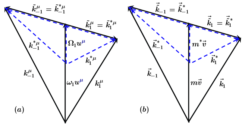
Figure 1: The definition of the various momentum possibilities discussed above (where the index 1 was chosen for simplicity), and the illustration of the dependence of the back-to-back momentum pairs on the four-velocity and on the mass-shift, is shown in (a) using relativistic notation. Solid lines represent the locally back-to-back momentum pair and its components for asymptotic quanta; dashed lines represent the same for in-medium modified, mass-shifted quanta. In (b), the analogous situation is illustrated using the non-relativistic notation.

Using the above expressions, the squeezing parameter can be evaluated as

$$f_{i,j}(x)=\frac{1}{2}\log\left[\frac{K^{\mu}_{i,j}(x)\,u_{\mu}(x)}{K^{*\nu}_{i,j}(x)\,u_{\nu}(x)}\right]=\frac{1}{2}\log\left[\frac{\omega_{{\mathbf{k}}_{i}}(x)+\omega_{{\mathbf{k}}_{j}}(x)}{\Omega_{{\mathbf{k}}_{i}}(x)+\Omega_{{\mathbf{k}}_{j}}(x)}\right]\equiv f_{\pm i,\pm j}(x),$$ (26)

where the spatial coordinate dependence enters through the position dependence of either the four-velocity or the in-medium mass modification, or both. However, it does not matter which of the locally back-to-back momenta are used for the evaluation of the amount of squeezing.

In this paper, we focus on the effects of expansion on the back-to-back correlations - or, with other words, does the flow wash out the signal for these correlations or not? Although the formalism of the squeezed back-to-back correlations was worked out with expanding systems in Ref. 2, no detailed investigations were performed to quantitatively study e.g. the strength of the signal with varying the strength of the flow.

Here we intend to investigate this question in one of the simplest geometrical cases. For the sake of clarity, we evaluate the flow effects for a non-relativistically expanding, spherically symmetric fireball, that freezes out at a constant temperature $T$ and has a Gaussian density profile. In this sense, we adopt the model emission function of Ref.Csorgo:fg , that was developed to study single particle spectra and Bose-Einstein (HBT) correlation functions in the simplest possible case of expanding systems. Later on it has been realized, that this emission function corresponds to the simplest member of a new family of exact solutions of non-relativistic hydrodynamicsCsorgo:c , which can be generalized in a straightforward manner to cylindrically and ellipsoidally symmetricCsorgo:d expansions, as well as to the case of relativistic expansions Csorgo:e , and in all cases, systems that expand with inhomogeneous temperature profiles Csorgo:d ; Csorgo:f .

Before investigating in detail the effects of various kind of inhomogeneities in the flow profiles and in the temperature profiles, let us turn our attention to the non-relativistic limit adopting the simplest possible scenario for the expansion that leads to analytic forms Csorgo:fg ; Csorgo:c .

For the sake of clarity, we present the explicit expressions in the non-relativistic limit of the above quantities, which is the appropriate limit for our non-relativistic flow model. Writing $u^{\mu}=\gamma(1,{\mathbf{v}})$ and using $\gamma=(1-{\mathbf{v}}^{2})^{-1/2}\approx 1+{\mathbf{v}}^{2}/2\approx 1$, we have that Eq. (22) leads to

$${\mathbf{k}}_{i}-m{\mathbf{v}}={\mathbf{k}}^{*}_{i}-m_{*}{\mathbf{v}},$$ (27)

and therefore

$${\mathbf{k}}_{\pm i}({\mathbf{r}}) = m\,{\mathbf{v}}({\mathbf{r}})\mp m\,{\mathbf{v}}({\mathbf{r}})\pm{\mathbf{k}}_{i},$$ (28)

$${\mathbf{k}}^{*}_{\pm i}({\mathbf{r}}) = m_{*}\,{\mathbf{v}}({\mathbf{r}})\mp m_{*}\,{\mathbf{v}}({\mathbf{r}})\pm{\mathbf{k}}^{*}_{i}.$$ (29)

With this, we obtain

$$K^{*\mu}_{i,j}(x)\,u_{\mu}\approx m_{*}+\frac{1}{2m_{*}}\left\{[{\mathbf{K}}^{*}_{i,j}-m_{*}{\mathbf{v}}({\mathbf{r}})]^{2}+\frac{1}{4}({\mathbf{q}}^{*}_{i,j})^{2}\right\},$$ (30)

where the total and relative local in-medium momenta are given by

$${\mathbf{K}}^{*}_{1,2}({\mathbf{r}})=\frac{1}{2}({\mathbf{k}}_{1}+{\mathbf{k}}_{2})+(m_{*}-m)\,{\mathbf{v}}({\mathbf{r}})\,, {\mathbf{q}}_{1,2}^{*}({\mathbf{r}})=({\mathbf{k}}_{1}-{\mathbf{k}}_{2})$$ (31)

$${\mathbf{K}}^{*}_{1,-2}({\mathbf{r}})=m_{*}{\mathbf{v}}({\mathbf{r}})+\frac{1}{2}({\mathbf{k}}_{1}-{\mathbf{k}}_{2})\,, {\mathbf{q}}^{*}_{1,-2}({\mathbf{r}})=-2m{\mathbf{v}}({\mathbf{r}})+({\mathbf{k}}_{1}+{\mathbf{k}}_{2})$$ (32)

$${\mathbf{K}}^{*}_{-1,2}({\mathbf{r}})=m_{*}{\mathbf{v}}({\mathbf{r}})-\frac{1}{2}({\mathbf{k}}_{1}-{\mathbf{k}}_{2})\,, {\mathbf{q}}^{*}_{-1,2}({\mathbf{r}})=2m{\mathbf{v}}({\mathbf{r}})-({\mathbf{k}}_{1}+{\mathbf{k}}_{2})$$ (33)

$${\mathbf{K}}^{*}_{-1,-2}({\mathbf{r}})=(m_{*}+m){\mathbf{v}}({\mathbf{r}})-\frac{1}{2}({\mathbf{k}}_{1}+{\mathbf{k}}_{2})\,, {\mathbf{q}}^{*}_{-1,-2}({\mathbf{r}})=-({\mathbf{k}}_{1}-{\mathbf{k}}_{2}).$$ (34)

The unstarred ${\mathbf{K}}_{i,j}$ and ${\mathbf{q}}_{i,j}$ momenta are obtained from the above by replacing $m_{*}$ by $m$ in these expressions. Note that ${\mathbf{q}}^{*}_{i,j}={\mathbf{q}}_{i,j}$, as it should be. These relations imply, that in the non-relativistic limit,

$${\mathbf{K}}^{*}_{ij}-m_{*}{\mathbf{v}}={\mathbf{K}}_{ij}-m{\mathbf{v}}.$$ (35)

In discussing finite-size effects, we distinguish between the volume of the entire thermalized medium, denoted by $V$, and the volume filled with mass-shifted quanta, denoted by $V_{s}$. Naturally, $V_{s}\leq V$ in the general case. In the derivation of the expressions for $G_{c}(1,2)$ and $G_{s}(1,2)$, for simplicity, we introduce a Gaussian profile function in the integrands, i.e., we consider that the volumetric region where the mass $m_{*}$ is significantly modified is smooth and Gaussian in shape. In other words, instead of considering a particular domain of integration, we perform the spatial integrals for $G_{c}(1,2)$ and $G_{c}(1,2)$ using a Gaussian weight $e^{-{\mathbf{r}}^{2}/2R_{s}^{2}}$ in the integrands, extending the integration region to infinity. Specifically, we have for $G_{c}(1,2)$ and $G_{s}(1,2)$

$$G_{c}({{\mathbf{k}}_{1}},{{\mathbf{k}}_{2}}) = \frac{E_{1,2}}{(2\pi)^{3}}\int d^{3}r\,e^{-i({\mathbf{k}}_{1}-{\mathbf{k}}_{2}){\bf\cdot}{\mathbf{r}}}\Biggl{\{}e^{-{\mathbf{r}}^{2}/2R_{s}^{2}}\,\Biggl{(}|c(1,2)|^{2}n^{*}_{1,2}(x)$$ (36)

$$+ |s(-1,-2)|^{2}\left[n^{*}_{-1,-2}(x)+1\right]\Biggr{)}+\left(1-e^{-{\mathbf{r}}^{2}/2R_{s}^{2}}\right)\;n_{1,2}(x)\Biggr{\}},$$

$$G_{s}({{\mathbf{k}}_{1}},{{\mathbf{k}}_{2}}) = \frac{E_{1,2}}{(2\pi)^{3}}\int d^{3}r\;e^{-i({\mathbf{k}}_{1}+{\mathbf{k}}_{2})\cdot{{\mathbf{r}}}}e^{-{\mathbf{r}}^{2}/2R_{s}^{2}}\Biggl{(}s^{*}(-1,2)\,c(2,-1)\;n^{*}_{-1,2}(x)$$ (37)

$$+ c(1,-2)\,s^{*}(-2,1)\,\left[1+n^{*}_{1,-2}(x)\right]\Biggr{)},$$

where $n^{*}_{i,j}(x)$ means that the local distribution function is to be evaluated with in-medium momenta, i.e. $n^{*}_{i,j}(x)\equiv n(x,K^{*}_{i,j})$. The integral over the factor $\left(1-e^{-{\mathbf{r}}^{2}/2R_{s}^{2}}\right)$ represents the integration over the region where there is no mass shift, corresponding to the region $V-V_{s}$. In this region, we have that the squeezing factors become $c(i,j)\rightarrow 1$ and $s(i,j)\rightarrow 0$.

In order to proceed, we need the expressions for $n^{*}(i,j)$ and $n(i,j)$. We consider their Boltzmann limit,

$$n(x,K_{i,j})\approx\exp{\left[-\frac{K^{\mu}_{i,j}u_{\mu}(x)-\mu(x)}{T(x)}\right]},$$ (38)

and the same for $n^{*}_{i,j}(x)$ with $K_{i,j}(x)$ replaced by $K^{*}_{i,j}(x)$. Considering that the chemical potential in the model of Ref. Csorgo:fg can be written as $\mu(x)/T(x)=\mu_{0}/T-{\mathbf{r}}^{2}/2R^{2}$, and making use of Eq. (30), it is easy to show that

$$n^{*}_{1,2}({\mathbf{r}}) = n^{*}_{0}~{}\exp\left\{{-\frac{{\mathbf{r}}^{2}}{2R^{2}}-\frac{\left[({\mathbf{k}}_{1}+{\mathbf{k}}_{2})/2-m\langle u\rangle{\mathbf{r}}/R\right]^{2}}{2m_{*}T}-\frac{({\mathbf{k}}_{1}-{\mathbf{k}}_{2})^{2}}{8m_{*}T}}\right\}$$ (39)

$$= n^{*}_{-1,-2}({\mathbf{r}})=n^{*}_{-1,2}({\mathbf{r}})=n^{*}_{1,-2}({\mathbf{r}}),$$

where

$$n^{*}_{0}=\exp\left(-\frac{m_{*}-\mu_{0}}{T}\right).$$ (40)

This factor is proportional to the mean multiplicity, and can be determined in principle from the absolute normalization of the single particle spectra. The corresponding unstarred $n_{i,j}({\mathbf{r}})$ are obtained from $n^{*}_{i,j}({\mathbf{r}})$ by replacing $m_{*}$ by $m$ in Eq. (39).

When evaluating the spectra and the correlations from this model, we realize that a mathematically equivalent problem has already been considered in Ref. Csorgo:fg . By replacing $m\rightarrow m_{*}$ and $t_{0}\rightarrow R_{G}m_{*}/\langle u\rangle m$ in the equations of Ref. Csorgo:fg , the results obtained there can be directly transcribed here.

Due to the equality in Eq. (35), we see that the accounting for the squeezing effects can be simplified for small mass shifts $(m_{*}-m)/m\ll 1$, such that the squeezing parameter can be written as

$$f(i,j,{\mathbf{r}})=\frac{1}{2}\log\left[\frac{K^{\mu}(i,j,x)\,u_{\mu}(x)}{K^{\nu}_{*}(i,j,x)\,u_{\nu}(x)}\right]\approx\frac{1}{2}\log\left(\frac{m}{m_{*}}\right).$$ (41)

The neglected terms are order of (kinetic energy/mass)² (masshift/mass)² and hence are of fourth order in small quantities. This limit is important, because in this case the coordinate dependence enters the squeezing parameter $f$ only through the possible position dependence of the mass-shift and so the flow effects on the squeezing parameter can be neglected. In principle, the position dependence of the mass shift can be calculated from thermal field models in the local density approximation. Therefore, in an approximation that the position dependence of the in-medium mass is neglected, the $c(i,j)=c_{0}$ and $s(i,j)=s_{0}$ factors can be removed from the integrands and all what remains to be done are Fourier transforms of Gaussian functions. The final result for $G_{c}$ and $G_{s}$ can be written as

$$G_{c}({{\mathbf{k}}_{1}},{{\mathbf{k}}_{2}}) = \frac{E_{1,2}}{(2\pi)^{3}}\Bigl{[}n^{*}_{0}\left(|c_{0}|^{2}+|s_{0}|^{2}\right)I^{c}_{1,2}(R_{s},R,T,m_{*})+|s_{0}|^{2}I^{c}_{1,2}(R_{s},\infty,\infty,m_{*})$$ (42)

$$+ n_{0}I^{c}_{1,2}(\infty,R,T,m)-n_{0}I^{c}_{1,2}(R_{s},R,T,m)\Bigr{]},$$

$$G_{s}({{\mathbf{k}}_{1}},{{\mathbf{k}}_{2}}) = \frac{E_{1,2}}{(2\pi)^{3}}\,c_{0}|\,s_{0}|\Bigl{[}\,2\,n^{*}_{0}\,I^{s}_{1,2}(R_{s},R,T,m_{*})+I^{s}_{1,2}(R_{s},\infty,\infty,m_{*})\Bigr{]},$$ (43)

where $I^{c}_{1,2}$ and $I^{s}_{1,2}$ are the resulting Fourier integrals

$$I^{c}_{1,2}(R_{s},R,T,m_{(*)}) = (2\pi\rho^{2}_{(*)})^{3/2}\exp\Biggl{\{}-\frac{({\mathbf{k}}^{2}_{1}+{\mathbf{k}}^{2}_{2})}{4m_{(*)}T}$$ (44)

$$- \frac{\rho^{2}_{(*)}}{2}\left[({\mathbf{k}}_{1}-{\mathbf{k}}_{2})+i\frac{m\langle u\rangle({\mathbf{k}}_{1}+{\mathbf{k}}_{2})}{2m_{(*)}TR}\right]^{2}\Biggr{\}},$$

$$I^{s}_{1,2}(R_{s},R,T,m_{*}) = (2\pi\rho^{2}_{*})^{3/2}\exp\Biggl{\{}-\frac{({\mathbf{k}}^{2}_{1}+{\mathbf{k}}^{2}_{2})}{4m_{*}T}-\frac{\rho^{2}_{*}}{2}\Biggl{[}1+i\frac{m\langle u\rangle}{2m_{*}TR}\Biggr{]}^{2}\left({\mathbf{k}}_{1}+{\mathbf{k}}_{2}\right)^{2}\Biggr{\}},$$ (45)

with

$$\frac{1}{\rho^{2}_{(*)}}\equiv\frac{1}{R^{2}_{s}}+\frac{1}{R^{2}}\left(1+\frac{m^{2}\langle u\rangle^{2}}{m_{(*)}T}\right).$$ (46)

Finally, we include finite-time emission effects in a schematic way using for the invariant function $F(\tau)$, that appears in the expression for $d^{4}\sigma^{\mu}(x)$, the following expression

$$F(\tau)=\frac{\theta(\tau-\tau_{0})}{\Delta t}\;e^{-(\tau-\tau_{0})/\Delta t},$$ (47)

where $\Delta t$ is a free parameter. This finishes the derivation of all the ingredients needed to evaluate $C_{2}({\mathbf{k}}_{1},{\mathbf{k}}_{2})$, Eq. (6). In the next section we will present numerical results.

IV Numerical Results

We present numerical results for two situations regarding the volumes over which mass modification occurs. In the first situation the mass shift occurs over the entire volume of the expanding system, i.e. $V_{s}=V$. This amounts to removing the factor $e^{-{\mathbf{r}}^{2}/2R_{s}^{2}}$ in Eqs. (36) and (37) or, equivalently, take $R_{s}\rightarrow\infty$ in $I^{c}$ and $I^{s}$. In the second situation, we consider $V_{s}<V$. In order to comply with the non-relativistic nature of the expansion model used in this paper, we present numerical results for the Back-to-Back Correlations of a $\phi$ meson pair. In free space, the $\phi$ meson mass is $m_{\phi}=1020$ MeV.

IV.1 Bulk decay of a volume filled with mass-shifted quanta

In this case, we suppose that the mass-shift occurs in the entire volume of the system, for simplicity considered here as a Gaussian with r.m.s. radius $R$. We will focus on the BBC correlation function, whose generic expression consists of the first and third terms on the right-hand-side of Eq. (6). The detailed expressions for the amplitudes are given in Appendix A. In what follows, we will concentrate on the value of momenta of the participant pair that maximizes the BBC signal, i.e., the case in which ${\mathbf{k}}_{1}=-{\mathbf{k}}_{2}={\mathbf{k}}$. The BBC correlation function can then be written as

$$C^{\sl max}_{BBC}({{\mathbf{k}}_{1}},{{\mathbf{k}}_{2}})=C_{BBC}({{\mathbf{k}}},-{{\mathbf{k}}})=1+\frac{|G_{s}({{\mathbf{k}}},-{{\mathbf{k}}})|^{2}}{G_{c}({{\mathbf{k}}},{{\mathbf{k}}})G_{c}(-{{\mathbf{k}}},-{{\mathbf{k}}})}=1+\frac{|G_{s}({{\mathbf{k}}},-{{\mathbf{k}}})|^{2}}{\left[G_{c}({{\mathbf{k}}},{{\mathbf{k}}})\right]^{2}}\;.$$ (48)

In the above equation, we have used the fact that the single-inclusive distribution, $G_{c}({{\mathbf{k}}},{{\mathbf{k}}})=G_{c}(-{{\mathbf{k}}},-{{\mathbf{k}}})$ depends only on the absolute value of the momentum, as can be seen in Eq. (60). With the aid of this equation, as well as of Eq. (58), the expression of the BBC correlation function is finally written as

$$C^{V}_{BBC}({{\mathbf{k}}},-{{\mathbf{k}}}) = 1+\big{|}c_{0}\;s_{0}\big{|}^{2}\,\Bigg{|}\frac{2n^{*}_{0}\;R_{*}^{3}\exp(-{\mathbf{k}}^{2}/2m_{*}T)+R^{3}\;}{n^{*}_{0}R_{*}^{3}\left(|c_{0}|^{2}+|s_{0}|^{2}\right)\exp(-{\mathbf{k}}^{2}/2m_{*}T_{*})+R^{3}|s_{0}|^{2}}\Bigg{|}^{2},$$ (49)

where

$$\frac{1}{R_{*}^{2}}=\frac{1}{R^{2}}\left(1+\frac{m^{2}\langle u\rangle^{2}}{m_{*}T}\right),\hskip 28.45274ptT_{*}=T+\frac{m^{2}}{m_{*}}\langle u\rangle^{2},$$ (50)

as given in Table 1 of Appendix A. The quantities $R_{*}$ and $T_{*}$ are, respectively, the flow-modified radius and the flow-modified temperature of the system where the mass-shift occurs in the entire volume.

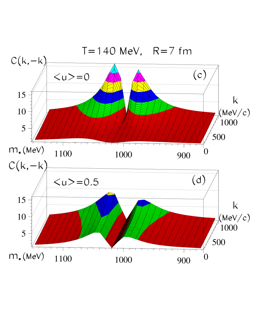
Figure 2: The Back-to-Back Correlation is shown as a function of the shifted mass $m_{*}$ on the left panels, and as a function of both $m_{*}$ and the momentum of each particle (${\mathbf{k}}_{1}=-{\mathbf{k}}_{2}={\mathbf{k}}$) on the right ones, for $R=7$ fm/c, $T=140$ MeV and $\Delta t=2$ fm/c. The plots (a) and (b) illustrate better the behavior of the BBC signal seen on the right panel, when $|{\mathbf{k}}|=500$ MeV/c and for $|{\mathbf{k}}|=1000$ MeV/c, respectively. In both cases, the dashed curve corresponds to $\langle u\rangle=0$ and the solid curve, to $\langle u\rangle=0.5$. In (c), it is shown the 3-D plot corresponding to the no flow case, with $\langle u\rangle=0$, whereas in (d), a radial flow with $v=\langle u\rangle r/R=0.5$ was considered.

In Fig. 2 we present the results for $C^{V}_{BBC}$ for $T=140$ MeV, $R=7$ fm and a finite emission time $\Delta t=2$ fm/c, for two different flow values. We clearly see in this figure that the presence of a radial flow causes the BBC correlation to be higher than the case with no flow in the low momentum region and for the same values of $m_{*}$ and ${\mathbf{k}}_{1}=-{\mathbf{k}}_{2}={\mathbf{k}}$, but it grows more slowly than in the no-flow case for increasing values of ${\mathbf{k}}$ and same $m_{*}$. We also see that for a flow of $\langle u\rangle=0.5$, the BBC signal increases for values of the momenta $|{\mathbf{k}}|\lesssim 1000$ MeV/c, but the no-flow case surpasses the previous case for $|{\mathbf{k}}|\gtrsim 1000$ MeV/c. This conclusion is more easily achieved by looking into the right panel of Fig. 2. The inversion of the BBC behavior for that value of ${\mathbf{k}}$ roughly coincides with the limit of applicability of our non-relativistic approximation. This result is very stimulating, suggesting that we would have bigger chances of observing the BBC effect in the lower $|{\mathbf{k}}|$ side of the the $BBC\times m_{*}\times|{\mathbf{k}}|$ region.

Figure 3: The effect of a finite emission interval on the Back to Back correlation function, as compared to instant emission, is illustrated in the left panel. The dashed curves have been reduced by a factor of $400$, and the solid curves correspond to the suppression by a finite emission duration, of about $\Delta t\simeq 2$ fm/c. The plot in (a) shows this effect in the absence of flow, already discussed in our previous paper. The plot in (b) shows the corresponding result when flow is included, with $<\!\!u\!\!>\!=0.5$ (the other parameters adopted to produce the curves are $R=7$ fm/c, $T=140$ MeV and $\Delta t=2$ fm/c. In part (c), we fixed the other parameters and study the influence of increasing values of $|{\mathbf{k}}|$ (the dashed curve corresponding to $|{\mathbf{k}}|=500$ MeV/c and the solid one, to $|{\mathbf{k}}|=500$ MeV/c). Finally, the plot in (d) considers the variation of the BBC curve for increasing values of $|{\mathbf{k}}|$, as indicated by the arrows, keeping all the other variables fixed to their values above.

In Fig. 3 we present results for different combinations of temperatures and flow velocities and emission times. We see again that flow enhances the BBC correlation function for small values of $|{\mathbf{k}}|$. The effect of the temperature is such that the BBC signal is stronger for lower values of $T$, and decreases the signal for higher values of $T$.

IV.2 Decay of a volume partly filled with mass-shifted quanta

Here we consider the scenario in which the mass shift of the bosons occurs in part of the system volume only. In this case, the expression for the BBC correlation function is more complex, even in the simpler limit of the maximal effect, i.e., when ${\mathbf{k}}_{1}=-{\mathbf{k}}_{2}={\mathbf{k}}$. The expression of $C^{\sl max}_{BBC}$ can again be obtained from Eq. (48), but this time we must replace the amplitudes by the expressions of Eqs. (70) and (71) of Appendix B, in the limit that the particles are back-to-back. In this case, we must use for the squeezing parameters in the region where there is no medium modification their appropriate limiting values

$$\lim\limits_{m_{*}\rightarrow m}\left(\begin{array}[]{c}c_{0}\\ s_{0}\\ \end{array}\right)\longrightarrow\left(\begin{array}[]{c}1\\ 0\\ \end{array}\right).$$ (51)

With this, we obtain after a long but straightforward calculation the expression

$$C^{2V}_{BBC}({{\mathbf{k}}},-{{\mathbf{k}}}) = 1+\Big{|}c_{0}\;s_{0}\Big{|}^{2}\;\Big{|}2n^{*}_{0}\;\rho_{*}^{3}\;\exp\!\!\left(-\frac{{\mathbf{k}}^{2}}{2m_{*}T}\right)+R_{s}^{3}\Big{|}^{2}\times$$

$$\Biggl{\{}n_{0}^{*}\;\rho_{*}^{3}\left(|c_{0}|^{2}+|s_{0}|^{2}\right)\exp{\left(-\frac{(R^{2}+R_{{}_{s}}^{2}){\mathbf{k}}^{2}}{2m_{*}(R^{2}T+R_{{}_{s}}^{2}T_{*})}\right)}+R_{s}^{3}|s_{0}|^{2}$$

$$+ n_{0}{\tilde{\cal R}}^{3}\exp{\left(-\frac{{\mathbf{k}}^{2}}{2m\tilde{\cal T}}\right)}-n_{0}{\tilde{\rho}}^{3}\exp{\left(-\frac{(R^{2}+R{{}_{s}}^{2}){\mathbf{k}}^{2}}{2m(R^{2}T+R{{}_{s}}^{2}\tilde{\cal T})}\right)}\Biggr{\}}^{-2},\;$$

where the parameters $\tilde{\cal T}=T+m\langle u\rangle^{2}$, $\tilde{\cal R}^{-2}=R^{-2}\left(1+m\langle u\rangle^{2}/T\right)$, $\tilde{\rho}^{-2}=\tilde{\cal R}^{-2}+R_{s}^{-2}$, $\rho_{*}^{-2}=R^{-2}\left(1+m^{2}\langle u\rangle^{2}/m_{*}T\right)+R_{s}^{-2}$ are given in Table 2 of Appendix B. The two are, respectively, the flow-modified temperature and the flow-modified radius in the region of no mass-shift. On the other hand, $\tilde{\rho}$ and $\rho_{*}$ are effective radius parameters corresponding to the no mass-shift region and the region where the mass-shift occurred, respectively. We see that they are functions of the flow parameter $\langle u\rangle$ and the parameter $R_{s}$, which corresponds to the radius of the mass-shift region. The parameter $T_{*}=T+m^{2}\langle u\rangle^{2}/m_{*}$, is the same as before, also written in Table 1 of Appendix A.

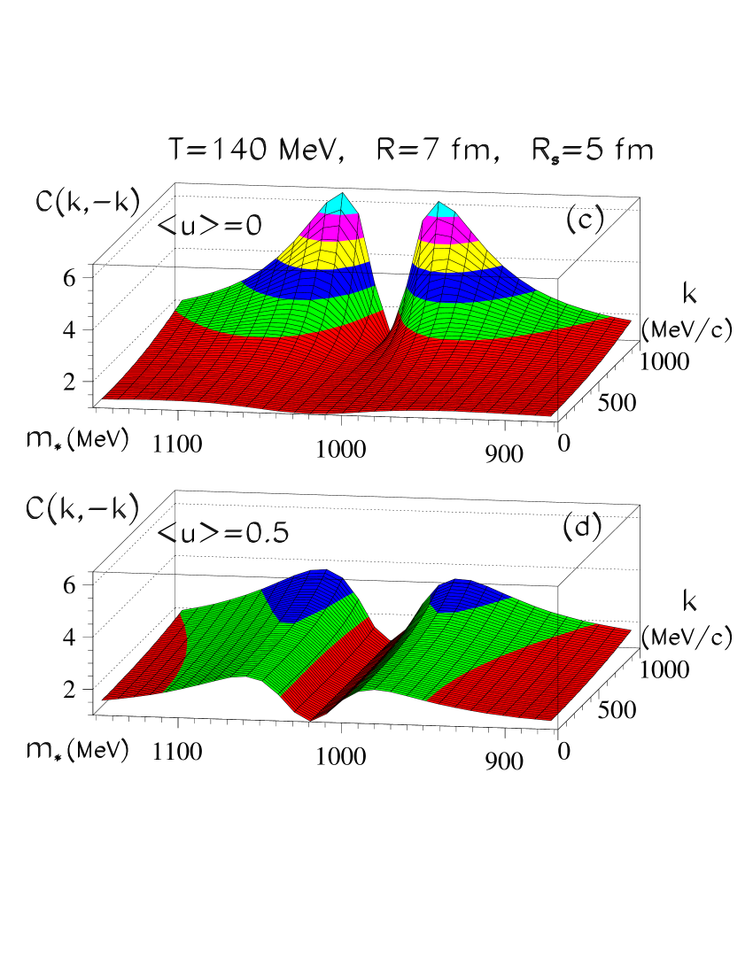
Figure 4: The plots in this panel are similar to the ones on Fig. 2. The main difference is that here we assumed that the mass-shift occurred only in a smaller part of the system volume. Here, the back-to-back correlation is shown as a function of the shifted mass $m_{*}$ on the right panel, and as function of both $m_{*}$ and the momentum of each particle (${\mathbf{k}}_{1}=-{\mathbf{k}}_{2}={\mathbf{k}}$), on the left ones, for $R=7$ fm/c, $R_{s}=5$ fm/c, $T=140$ MeV and $\Delta t=2$ fm/c. The plots in parts (a) and (b) illustrate better the behavior of the BBC signal seen in parts (c) and (d), for $|{\mathbf{k}}|=800$ MeV/c and for $|{\mathbf{k}}|=1000$ MeV/c. In both cases, the dashed curve corresponds to $\langle u\rangle=0$ and the solid curve, to $\langle u\rangle=0.5$. In the 3-D plot in (c), no flow ($\langle u\rangle=0$) was considered, whereas a radial flow with $v=\langle u\rangle r/R=0.5$ was included in the (d) plot.

Similarly to Eq. (49), the above Eq. (LABEL:BBCcorr2Vf) has also very interesting limiting cases. The first one is the case of vanishing squeezing, $m_{*}\rightarrow m$, which implies that $|s_{0}|\rightarrow 0$ and $|c_{0}|\rightarrow 1$, and the squeezed Back-to-Back Correlations vanish.

The large momentum limit is also very interesting. In this case, the exponential, thermal contributions disappear, and the surviving terms come from the decay of the squeezed vacuum to the asymptotic quanta. Both the numerator and the denominator of Eq. (LABEL:BBCcorr2Vf) will be proportional to the square of the squeezed volume, hence Eq. (LABEL:BBCcorr2Vf) and Eq. (49) will be reduced to a form similar to

$$C(k,-k)=1+|c_{0}/s_{0}|^{2}$$

which has no upper limit, and diverges for small but non-vanishing amount of squeezing, where $|c_{0}|\rightarrow 1$ and $|s_{0}|\rightarrow 0$. This property, the unlimited strength of the squeezed BBC-s – even if the mass modification does not happen in the whole volume – makes it worthwhile to look for these effects experimentally as signals of in-medium mass modifications. Again, for large in medium mass modifications and large momenta, the strength of the squeezed BBC-s will be similar to that of the HBT effect:

$$C(k,-k)\rightarrow 2$$

if $|c_{0}|,|s_{0}|\rightarrow\infty$, as in this limit, $|c_{0}|/|s_{0}|\rightarrow 1$.

The single particle spectra also behaves interestingly in these limits, which is discussed in Appendices A and B.

In Fig. 4 we show the BBC correlation corresponding to the hypothesis that the mass-shift occurred only in a smaller part of the system volume. We see a very close similarity to the results corresponding to the mass-shift occurring in the entire system volume, shown in Fig. 2. The major difference between the two of them is that in Fig. 4 the correlation signal is lower, as expected, since a the mass-shift occurred in a smaller volume in this case.

V Conclusions and Future Perspectives

In this paper we discussed the effects of the system expansion and flow on the back-to-back correlation, also limiting the system to a more realistic finite size. For simplicity, we restricted our analysis to the non-relativistic domain. In our study, we have also considered that the flow effects on the squeezing parameter were negligible. For simplicity, we have also assumed a 3-D Gaussian profile for the system. We showed here the effects of the decoupling temperature on the BBC signal, fixing all other parameters, as in the bottom right plot of Fig. 3. In this case, we observed that the BBC signal survives stronger if the decoupling temperature is lower. Fixing $T$ and the other parameters, we also showed the effect of increasing momentum on the signal survival. More striking, we showed in Figures 2 and 4 the conclusion about the best region for looking into the BBC effect in the $m_{*}\times|{\mathbf{k}}|$ plane: the search for the signal is more pronounced in the small $|{\mathbf{k}}|$ region, when we are to take into account the system expansion and the presence of moderate to strong flow. For higher values of $|{\mathbf{k}}|$, the BBC signal would be more pronounced if the system flow could be neglected. In any case, what remains as the most encouraging point coming out of our present study is that the BBC seems to survive with measurable intensity in the more realistic situation of finite size systems subjected to hydrodynamical expansion and consequent flow.

Appendix A Mass-shifted in the entire volume

It turns out that the formalism can be presented in the simplest manner if we assume, that the whole thermalized medium is filled with mass-shifted quanta, and that the whole medium decays suddenly to asymptotic quanta. This case is the subject of this appendix. It is also possible, that e.g. due to density inhomogeneities, the volume where the mass-shift is non-zero is different (smaller) than the totality of the volume filled out by thermalized quanta. This case will be investigated in the next appendix.

For the case of non-relativistic hydrodynamics, assuming for the sake of simplicity a sudden freeze-out, $\int d^{4}\Sigma_{\mu}K^{\mu}_{ij}=\int d^{3}{\mathbf{r}}\int dt\delta(t-t_{0})E_{ij}=E_{ij}\int d^{3}{\mathbf{r}}$, the chaotic and the squeezed amplitudes are easily obtained from the ones previously derived in Eq. (42) and (43) by taking the limit $R_{s}\rightarrow\infty$ in those equations as well as in all the others that immediately follow them, i.e., Eq. (44), (45), and (46). The intuitive way to understand this limit is to consider the mass-shift region as extended so as to include the entire volume of the system, by simply taking the limit $R_{s}\rightarrow\infty$. The volume of the system, however, will be still delimited by the Gaussian profile with rms $R$. In this limit, the last two terms in Eq.(42) exactly cancel, since

$$\lim\limits_{R_{s}\rightarrow\infty}I^{c}_{1,2}(R_{s},R,\langle u\rangle,m)=I^{c}_{1,2}(\infty,R,\langle u\rangle,m).$$ (53)

Consequently, the effective squeezing region becomes $R_{s}\rightarrow R$.

Before writing the resulting expression for $G_{c}(1,2)$, $G_{s}(1,2)$ and $G_{c}(i,i)$, it is usefull to define two parameters in terms of which we can write those expressions, i.e., the flow-modified temperature $T_{*}$ and the flow-modified radius of the single volume case

$$R_{*}=\lim\limits_{R_{s}\rightarrow\infty}\rho(R_{s},R,m_{(*)})$$ (54)

as given in Eq. (46). We can then write the chaotic amplitude, $G_{c}({\mathbf{k}}_{1},{\mathbf{k}}_{2})$ as

$$G^{1V}_{c}({\mathbf{k}}_{1},{\mathbf{k}}_{2}) = \lim\limits_{R_{s}\rightarrow\infty}\left\{\frac{E_{1,2}}{(2\pi)^{3}}\Bigr{[}n^{*}_{0}\left(|c_{0}|^{2}+|s_{0}|^{2}\right)I^{c}_{1,2}(R_{s},R,T,m_{*})+|s_{0}|^{2}I^{c}_{1,2}(R_{s},R,\infty,m_{*})\Bigr{]}\right\}$$ (55)

$$= \frac{E_{1,2}}{(2\pi)^{3}}|s_{0}|^{2}(2\pi R^{2})^{3/2}\exp\left[-\frac{R^{2}}{2}({\mathbf{k}}_{1}-{\mathbf{k}}_{2})^{2}\right]$$

$$+ \frac{E_{1,2}}{(2\pi)^{3}}n^{*}_{0}\left(|c_{0}|^{2}+|s_{0}|^{2}\right)$$

$$\times (2\pi R_{*}^{2})^{3/2}\exp\left\{-\frac{({\mathbf{k}}^{2}_{1}+{\mathbf{k}}^{2}_{2})}{4m_{*}T}-\frac{R_{*}^{2}}{2}\left[({\mathbf{k}}_{1}-{\mathbf{k}}_{2})+i\frac{m\langle u\rangle({\mathbf{k}}_{1}+{\mathbf{k}}_{2})}{2m_{*}TR}\right]^{2}\right\}.$$

We can rearrange the above terms in a more compact form, and explicitly writing in terms of the variables defined in Table 1 (from which we can see that $R^{2}_{*}/RT=R/T_{*}$) we have

$$G^{1V}_{c}({\mathbf{k}}_{1},{\mathbf{k}}_{2}) = \frac{E_{1,2}}{(2\pi)^{3/2}}R^{3}|s_{0}|^{2}\exp\left[-\frac{R^{2}}{2}({\mathbf{k}}_{1}-{\mathbf{k}}_{2})^{2}\right]$$ (56)

$$+ \frac{E_{1,2}n^{*}_{0}}{(2\pi)^{3}}\;(|c_{0}|^{2}+|s_{0}|^{2})\;(2\pi R^{2}_{*})^{3/2}\exp\left[-\frac{({\mathbf{k}}_{1}+{\mathbf{k}}_{2})^{2}}{8m_{*}T_{*}}\right]$$

$$\times \exp\left[-\frac{im\langle u\rangle R}{2m_{*}T_{*}}({\mathbf{k}}_{1}^{2}-{\mathbf{k}}_{2}^{2})-\left(\frac{1}{8m_{*}T}+\frac{R_{*}^{2}}{2}\right)({\mathbf{k}}_{1}-{\mathbf{k}}_{2})^{2}\right].$$

Table 1: Parameters used in the single volume case.

Parameter	Relation to other parameters	Integral results where they appear
$T_{*}$	$T_{*}=T+\frac{m^{2}}{m_{*}}\langle u\rangle^{2}$	$I^{c}_{i,j}(\infty,R,T,m_{*})$
$R_{*}$	$R_{*}^{-2}=R^{-2}\left(1+\frac{m^{2}\langle u\rangle^{2}}{m_{*}T}\right)$	$I^{s}_{i,j}(\infty,R,T,m_{*})$

The coherent amplitude $G_{s}({\mathbf{k}}_{1},{\mathbf{k}}_{2})$ can be written as

$$G^{1V}_{s}({\mathbf{k}}_{1},{\mathbf{k}}2) = \lim\limits_{R_{s}\rightarrow\infty}\left\{\frac{E_{1,2}}{(2\pi)^{3}}\,c_{0}|s_{0}|\Bigl{[}2\,n^{*}_{0}I^{s}_{1,2}(R_{s},R,T,m_{*})+I^{s}_{1,2}(R_{s},R,\infty,m_{*})\Bigr{]}\right\}$$ (57)

$$= \frac{E_{1,2}}{(2\pi)^{3}}c_{0}|s_{0}|(2\pi R^{2})^{3/2}\exp\left[-\frac{R^{2}}{2}({\mathbf{k}}_{1}+{\mathbf{k}}_{2})^{2}\right]+\frac{E_{1,2}n^{*}_{0}}{(2\pi)^{3}}\,2c_{0}|s_{0}|$$

$$\times (2\pi R_{*}^{2})^{3/2}\,\exp\left[-\frac{({\mathbf{k}}^{2}_{1}+{\mathbf{k}}^{2}_{2})}{4m_{*}T}-\frac{R_{*}^{2}}{2}\left(1+i\frac{m\langle u\rangle}{2m_{*}TR}\right)^{2}\left({\mathbf{k}}_{1}+{\mathbf{k}}_{2}\right)^{2}\right].$$

Similarly to what was done before, can also rewrite the expression for $G_{s}({\mathbf{k}}_{1},{\mathbf{k}}_{2})$ explicitly in terms of the variables defined in Table 1, leading to

$$G^{1V}_{s}({\mathbf{k}}_{1},{\mathbf{k}}_{2}) = \frac{E_{1,2}}{(2\pi)^{3}}c_{0}|s_{0}|(2\pi R^{2})^{3/2}\exp\left[-\frac{R^{2}}{2}({\mathbf{k}}_{1}+{\mathbf{k}}_{2})^{2}\right]$$ (58)

$$+ \frac{E_{1,2}n^{*}_{0}}{(2\pi)^{3/2}}\;(2\pi R^{2}_{*})^{3/2}\,(2\,c_{0}|s_{0}|)\,\exp\left[-\frac{({\mathbf{k}}_{1}-{\mathbf{k}}_{2})^{2}}{8m_{*}T}\right]$$

$$\times \exp\left[-\frac{im\langle u\rangle R}{2m_{*}T_{*}}({\mathbf{k}}_{1}+{\mathbf{k}}_{2})^{2}-\left(\frac{1}{8m_{*}T_{*}}+\frac{R_{*}^{2}}{2}\right)({\mathbf{k}}_{1}+{\mathbf{k}}_{2})^{2}\right].$$

Also, the single-particle distribution, the amplitude appearing in the denominator of both the BBC and the HBT correlation functions can be written as

$$N^{1V}_{1}({\bf k}_{i}) = G^{1V}_{c}({\mathbf{k}}_{i},{\mathbf{k}}_{i})$$

$$= \lim\limits_{R_{s}\rightarrow\infty}\frac{E_{i,i}}{(2\pi)^{3}}\Bigr{[}n^{*}_{0}\left(|c_{0}|^{2}+|s_{0}|^{2}\right)I^{c}_{i,i}(R_{s},R,T,m_{*})+|s_{0}|^{2}I^{c}_{i,i}(R_{s},R,\infty,m_{*})\Bigr{]}$$

$$= \frac{E_{i,i}}{(2\pi)^{3}}|s_{0}|^{2}(2\pi R^{2})^{3/2}$$

$$+ \frac{E_{i,i}n^{*}_{0}}{(2\pi)^{3}}\left(|c_{0}|^{2}+|s_{0}|^{2}\right)(2\pi R_{*}^{2})^{3/2}\exp\left[-\frac{{\mathbf{k}}^{2}_{i}}{2m_{*}T}+\frac{R_{*}^{2}}{2}\left(\frac{m\langle u\rangle{\mathbf{k}}_{i}}{m_{*}TR}\right)^{2}\right]$$

Analogously, we can rewrite $G_{c}({\mathbf{k}}_{i},{\mathbf{k}}_{i})$ explicitly in terms of $T_{*}$ and $R_{*}$, as

$$N^{1V}_{1}({\bf k}_{i}) = G^{1V}_{c}({\mathbf{k}}_{i},{\mathbf{k}}_{i})$$ (60)

$$= \frac{E_{i,i}}{(2\pi)^{3}}|s_{0}|^{2}(2\pi R^{2})^{3/2}+\frac{E_{i,i}n^{*}_{0}}{(2\pi)^{3/2}}\left(|c_{0}|^{2}+|s_{0}|^{2}\right)(2\pi R^{2}_{*})^{3/2}\exp\left(-\frac{{\mathbf{k}}^{2}_{i}}{2m_{*}T_{*}}\right).$$

Let us investigate the vanishing squeezing and the large momentum limits of the single particle spectra, similarly to the analysis of the correlation functions as was done after Eq. (49).

In case of vanishing squeezing, $m_{*}\rightarrow m$, $|s_{0}|\rightarrow 0$ and $|c_{0}|\rightarrow 1$, hence we spectra will contain a thermal and a flow contribution, and we recover the results of Ref. Csorgo:fg . In the large momentum limit, for non-vanishing squeezing, rather surprisingly the single particle spectra becomes a constant. This corresponds to the decay of a modified vacuum with a fixed volume, described by the first term of (60). This is the direct consequence of our neglecting for the present purposes the position dependence of the in-medium mass modification. Also, this result implies that the squeezing mechanism not only makes strong signals in the back-to-back correlations, but there is also an interesting signal for squeezing in the single particle spectra.

Appendix B Mass-shifted in partial volume

If the mass-shift occurs only in a certain portion of volume $V_{s}$ of the whole system $V(>V_{s})$, the expressions for the amplitudes contain other terms besides the ones discussed in the Appendix A. Again, in order to avoid too much clutter it is useful to define appropriate flow-modified variables. However, in this case, we will need to define two sets of such parameters as flow-modified radii and temperatures, one set corresponding to the region where there is no mass-shift, which we will denote by $\tilde{\cal R}$, $\tilde{\rho}$, and $\tilde{\cal T}$, and another for the inside of the mass-shifted region, denoted by $R_{*}$ and $T_{*}$, this last one, naturally, being the same as defined in Table 1.

Table 2: Parameters used in the two-volume case.

Parameter	Relation to other parameters	Integral results where they appear
$\tilde{\cal T}$	$\tilde{\cal T}=T+m\langle u\rangle^{2}$	$I^{c}_{i,j}(\infty,R,T,m)$ & $I_{c}(R_{s},R,T,m)$
$\tilde{\cal R}$	$\tilde{\cal R}^{-2}=R^{-2}\left(1+\frac{m}{T}\langle u\rangle^{2}\right)$	$I^{c}_{i,j}(\infty,R,T,m)$
$\tilde{\rho}$	$\tilde{\rho}^{-2}=\tilde{\cal R}^{-2}+R_{s}^{-2}$	$I^{c}_{i,j}(R_{s},R,T,m)$
$T_{*}$	$T_{*}=T+\frac{m^{2}}{m_{*}}\langle u\rangle^{2}$	$I^{c}_{i,j}(R_{s},R,T,m_{*})$
$\rho_{*}$	$\rho_{*}^{-2}=R^{-2}\left(1+\frac{m^{2}\langle u\rangle^{2}}{m_{*}T}\right)+R_{s}^{-2}$	$I^{s}_{i,j}(R_{s},R,T,m_{*})$

In the case where the mass-shift occurs in a small portion of the system volume, $V_{s}<V$, the chaotic amplitude is given by Eq. (42) and (44), i.e.,

$$G^{2V}_{c}(1,2) = \frac{E_{1,2}}{(2\pi)^{3}}\Bigl{[}n^{*}_{0}\left(|c_{0}|^{2}+|s_{0}|^{2}\right)I^{c}_{1,2}(R_{s},R,T,m_{*})+|s_{0}|^{2}I^{c}_{1,2}(R_{s},\infty,\infty,m_{*})$$ (61)

$$+ n_{0}I^{c}_{1,2}(\infty,R,T,m)-n_{0}I^{c}_{1,2}(R_{s},R,T,m)\Bigr{]}.$$

Working out each of the integrals above separately, we have

$$I^{c}_{1,2}(R_{s},R,T,m_{*}) = (2\pi\rho_{*}^{2})^{3/2}\exp\left\{-\frac{({\mathbf{k}}^{2}_{1}+{\mathbf{k}}^{2}_{2})}{4m_{*}T}-\frac{\rho_{*}^{2}}{2}\left[({\mathbf{k}}_{1}-{\mathbf{k}}_{2})+i\frac{m\langle u\rangle({\mathbf{k}}_{1}+{\mathbf{k}}_{2})}{2m_{*}TR}\right]^{2}\right\}$$ (62)

$$= (2\pi\rho_{*}^{2})^{3/2}\exp\left[-i\frac{m\langle u\rangle\rho_{*}^{2}({\mathbf{k}}_{1}^{2}-{\mathbf{k}}_{2}^{2})}{2m_{*}RT}\right]$$

$$\times \exp{\left[-\left(\frac{1}{8m_{*}T}+\frac{\rho_{*}^{2}}{2}\right)({\mathbf{k}}_{1}-{\mathbf{k}}_{2})^{2}-\frac{(R^{2}+R_{{}_{s}}^{2})({\mathbf{k}}_{1}+{\mathbf{k}}_{2})^{2}}{8m_{*}(R^{2}T+R_{{}_{s}}^{2}T_{*})}\right]},$$

$$I^{c}_{1,2}(R_{s},\infty,\infty,m_{*}) = (2\pi R_{s}^{2})^{3/2}\exp\left[-\frac{R_{s}^{2}}{2}({\mathbf{k}}_{1}-{\mathbf{k}}_{2})^{2}\right],$$ (63)

$$I^{c}_{1,2}(\infty,R,T,m) = (2\pi\tilde{\cal R}^{2})^{3/2}\exp\left\{-\frac{({\mathbf{k}}^{2}_{1}+{\mathbf{k}}^{2}_{2})}{4mT}-\frac{\tilde{\cal R}^{2}}{2}\left[({\mathbf{k}}_{1}-{\mathbf{k}}_{2})+i\frac{m\langle u\rangle({\mathbf{k}}_{1}+{\mathbf{k}}_{2})}{2mTR}\right]^{2}\right\}$$ (64)

$$= (2\pi{\tilde{\cal R}}^{2})^{3/2}\exp\left[-i\frac{\langle u\rangle{\tilde{\cal R}}^{2}({\mathbf{k}}_{1}^{2}-{\mathbf{k}}_{2}^{2})}{2RT}\right]$$

$$\times \exp{\left[-\left(\frac{1}{8mT}+\frac{{\tilde{\cal R}}^{2}}{2}\right)({\mathbf{k}}_{1}-{\mathbf{k}}_{2})^{2}-\frac{({\mathbf{k}}_{1}+{\mathbf{k}}_{2})^{2}}{8m\tilde{\cal T}}\right]},$$

$$I^{c}_{1,2}(R_{s},R,T,m) = (2\pi\tilde{\rho}^{2})^{3/2}\exp\left\{-\frac{({\mathbf{k}}^{2}_{1}+{\mathbf{k}}^{2}_{2})}{4mT}-\frac{\tilde{\rho}^{2}}{2}\left[({\mathbf{k}}_{1}-{\mathbf{k}}_{2})+i\frac{m\langle u\rangle({\mathbf{k}}_{1}+{\mathbf{k}}_{2})}{2mTR}\right]^{2}\right\}$$ (65)

$$= (2\pi{\tilde{\rho}}^{2})^{3/2}\exp\left[-i\frac{\langle u\rangle{\tilde{\rho}}^{2}({\mathbf{k}}_{1}^{2}-{\mathbf{k}}_{2}^{2})}{2RT}\right]$$

$$\times \exp{\left[-\left(\frac{1}{8mT}+\frac{{\tilde{\rho}}^{2}}{2}\right)({\mathbf{k}}_{1}-{\mathbf{k}}_{2})^{2}-\frac{(R^{2}+R_{{}_{s}}^{2})({\mathbf{k}}_{1}+{\mathbf{k}}_{2})^{2}}{8m(R^{2}T+R_{{}_{s}}^{2}\tilde{\cal T})}\right]}.$$

Substituting these into Eq. (61), the complete expression for the chaotic amplitude can finally be written as

$$G^{2V}_{c}(1,2) = n_{0}^{*}\;\rho_{*}^{3}\left[|c_{0}|^{2}+|s_{0}|^{2}\right]\exp\left[-i\frac{m\langle u\rangle\rho_{*}^{2}({\mathbf{k}}_{1}^{2}-{\mathbf{k}}_{2}^{2})}{2m_{*}RT}\right]$$ (66)

$$\times \exp\left[-\left(\frac{1}{8m_{*}T}+\frac{\rho_{*}^{2}}{2}\right)({\mathbf{k}}_{1}-{\mathbf{k}}_{2})^{2}-\frac{(R^{2}+R_{{}_{s}}^{2})({\mathbf{k}}_{1}+{\mathbf{k}}_{2})^{2}}{8m_{*}(R^{2}T+R_{{}_{s}}^{2}T_{*})}\right]$$

$$+ \frac{E_{1,2}}{(2\pi)^{3/2}}R_{s}^{3}|s_{0}|^{2}\exp\left[-\frac{R_{s}^{2}}{2}({\mathbf{k}}_{1}-{\mathbf{k}}_{2})^{2}\right]$$

$$+ \frac{E_{1,2}n_{0}}{(2\pi)^{3}}\Biggl{\{}(2\pi{\tilde{\cal R}}^{2})^{3/2}\exp\left[-i\frac{\langle u\rangle{\tilde{\cal R}}^{2}({\mathbf{k}}_{1}^{2}-{\mathbf{k}}_{2}^{2})}{2RT}\right]$$

$$\times \exp{\left[-\left(\frac{1}{8mT}+\frac{{\tilde{\cal R}}^{2}}{2}\right)({\mathbf{k}}_{1}-{\mathbf{k}}_{2})^{2}-\frac{({\mathbf{k}}_{1}+{\mathbf{k}}_{2})^{2}}{8m\tilde{\cal T}}\right]}$$

$$- (2\pi{\tilde{\rho}}^{2})^{3/2}\exp\left[-i\frac{\langle u\rangle{\tilde{\rho}}^{2}({\mathbf{k}}_{1}^{2}-{\mathbf{k}}_{2}^{2})}{2RT}\right]$$

$$\times \exp\left[-\left(\frac{1}{8mT}+\frac{{\tilde{\rho}}^{2}}{2}\right)({\mathbf{k}}_{1}-{\mathbf{k}}_{2})^{2}-\frac{(R^{2}+R_{{}_{s}}^{2})({\mathbf{k}}_{1}+{\mathbf{k}}_{2})^{2}}{8m(R^{2}T+R_{{}_{s}}^{2}\tilde{\cal T})}\right]\Biggr{\}}$$

The coherent amplitude is given by Eqs. (43) and (45), as

$$G^{2V}_{s}({\mathbf{k}}_{1},{\mathbf{k}}2)=\frac{E_{1,2}}{(2\pi)^{3}}\,c_{0}|\,s_{0}|\Bigl{[}\,2\,n^{*}_{0}\,I^{s}_{1,2}(R_{s},R,T,m_{*})+I^{s}_{1,2}(R_{s},\infty,\infty,m_{*})\Bigr{]},$$ (67)

where

$$I^{s}_{1,2}(R_{s},R,T,m_{*}) = (2\pi\rho_{*}^{2})^{3/2}\exp\left\{-\frac{({\mathbf{k}}^{2}_{1}+{\mathbf{k}}^{2}_{2})}{4m_{*}T}-\frac{\rho_{*}^{2}}{2}\left[1+i\frac{m\langle u\rangle}{2m_{*}TR}\right]^{2}\left({\mathbf{k}}_{1}+{\mathbf{k}}_{2}\right)^{2}\right\}$$ (68)

$$= (2\pi\rho_{*}^{2})^{3/2}\;\exp{\left[-i\frac{m\langle u\rangle\rho_{*}^{2}({\mathbf{k}}_{1}+{\mathbf{k}}_{2})^{2}}{2m_{*}RT}\right]}$$

$$\times \exp{\left[-\frac{({\mathbf{k}}_{1}-{\mathbf{k}}_{2})^{2}}{8m_{*}T}-\frac{\rho_{*}^{2}}{2}({\mathbf{k}}_{1}+{\mathbf{k}}_{2})^{2}-\frac{(R^{2}+R_{{}_{s}}^{2})({\mathbf{k}}_{1}+{\mathbf{k}}_{2})^{2}}{8m_{*}(R^{2}T+R_{{}_{s}}^{2}T_{*})}\right]},$$

$$I^{s}_{1,2}(R_{s},\infty,\infty,m_{*}) = (2\pi R_{s}^{2})^{3/2}\exp\left[-\frac{R_{s}^{2}}{2}\left({\mathbf{k}}_{1}+{\mathbf{k}}_{2}\right)^{2}\right].$$ (69)

By substituting the above two terms, Eq. (68) and (69) into Eq. (67), we get the final form of the coherent amplitude

$$G^{2V}_{s}(1,2) = \frac{E_{1,2}}{(2\pi)^{3}}\,(2\pi R^{2}_{s})^{3/2}\,(c_{0}s_{0})\,\exp\left[-\frac{R_{s}^{2}}{2}({\mathbf{k}}_{1}+{\mathbf{k}}_{2})^{2}\right]$$ (70)

$$+ \frac{E_{1,2}n_{0}^{*}}{(2\pi)^{3}}\,(2\pi\rho^{2}_{*})^{3/2}\,(2c_{0}s_{0})\exp{\left[-i\frac{m\langle u\rangle\rho_{*}^{2}({\mathbf{k}}_{1}+{\mathbf{k}}_{2})^{2}}{2m_{*}RT}\right]}$$

$$\times \exp{\left[-\frac{({\mathbf{k}}_{1}-{\mathbf{k}}_{2})^{2}}{8m_{*}T}-\frac{\rho_{*}^{2}}{2}({\mathbf{k}}_{1}+{\mathbf{k}}_{2})^{2}-\frac{(R^{2}+R_{{}_{s}}^{2})({\mathbf{k}}_{1}+{\mathbf{k}}_{2})^{2}}{8m_{*}(R^{2}T+R_{{}_{s}}^{2}T_{*})}\right]}.$$

The single-particle distribution for this situation of two volumes can be written as

$$N^{2V}_{1}({\bf k}_{i}) = G^{2V}_{c}(i,i)$$ (71)

$$= \frac{E_{i,i}}{(2\pi)^{3}}\Bigl{[}n^{*}_{0}\left(|c_{0}|^{2}+|s_{0}|^{2}\right)I^{c}_{i,i}(R_{s},R,T,m_{*})+|s_{0}|^{2}I^{c}_{i,i}(R_{s},\infty,\infty,m_{*})$$

$$+ n_{0}I^{c}_{i,i}(\infty,R,T,m)-n_{0}I^{c}_{i,i}(R_{s},R,T,m)\Bigr{]}$$

$$= \frac{E_{i,i}}{(2\pi)^{3}}\Biggl{\{}(2\pi R^{2}_{s})^{3/2}|s_{0}|^{2}+n_{0}^{*}\;(2\pi\rho^{2}_{*})^{3/2}\left(|c_{0}|^{2}+|s_{0}|^{2}\right)\exp{\left[-\frac{(R^{2}+R_{{}_{s}}^{2}){\mathbf{k}}_{i}^{2}}{2m_{*}(R^{2}T+R_{{}_{s}}^{2}T_{*})}\right]}$$

$$+ n_{0}(2\pi{\tilde{\cal R}}^{2})^{3/2}\exp{\left(-\frac{{\mathbf{k}}_{i}^{2}}{2m\tilde{\cal T}}\right)}-n_{0}(2\pi{\tilde{\rho}}^{2})^{3/2}\exp{\left[-\frac{(R^{2}+R{{}_{s}}^{2}){\mathbf{k}}_{i}^{2}}{2m(R^{2}T+R{{}_{s}}^{2}\tilde{\cal T})}\right]}\Biggr{\}}.$$

Note again that in the large momentum region only the first term survives, which corresponds to a constant contribution given by the modified vacuum, and the size of this contribution is less than in case of Eq. (60), as the in-medium modified quanta do not fill the entire volume in the present case: $R_{s}<R$.

References

- (1) M. Asakawa and T. Csörgő, hep-ph/9612331, Heavy Ion Physics 4, (1996) 233; M. Asakawa and T. Csörgő, in proc. Strong and Electroweak Matter’97 Conference, Eger, Hungary, May 1997. (World Scientific, Singapore, 1998, F. Csikor and Z. Fodor eds.) p. 332 [quant-ph/9708006].
- (2) M. Asakawa, T. Csörgő and M. Gyulassy, Phys. Rev. Lett. 83, (1999) 4013.
- (3) P.K. Panda, T. Csörgő, Y. Hama, G. Krein, S.S. Padula, Phys. Lett. B512 (2001) 49.
- (4) A. Makhlin and Yu. Sinyukov, Sov. J. Nucl. Phys. 46, (1987) 354; Yad. Phys. 46, (1987) 637; Yu. Sinyukov, Nucl. Phys. A566, (1994) 598c.
- (5) M. Gyulassy, S. K. Kaufmann, and L. W. Wilson, Phys. Rev. C20 (1979) 2267
- (6) I. Andreev and R. Weiner, Phys. Lett. B373 (1996) 159.
- (7) T. Csörgő, B. Lörstad and J. Zimányi, Phys. Lett. B 338 (1994) 134 [nucl-th/9408022]; P. Csizmadia, T. Csörgő and B. Lukács, Phys. Lett. B 443 (1998) 21 [arXiv:nucl-th/9805006].
- (8) T. Csörgő, Cent.Eur.J.Phys.2:556-565,2004 [nucl-th/9809011].
- (9) T. Csörgő, F. Grassi, Y. Hama, T. Kodama Phys.Lett. B565 (2003) 107-115 [nucl-th/0305059].
- (10) T. Csörgő, L. P. Csernai, Y. Hama, T. Kodama, Heavy Ion Phys. A21 (2004) 73-84 [nucl-th/0306004].
- (11) T. Csörgő, hep-ph/0111139.