TUM-T39-05-15

Signatures of chiral dynamics in the Nucleon to Delta transition

Tobias A. Gail and Thomas R. Hemmert,

Theoretische Physik T39, Physik Department
TU-München, D-85747 Garching, Germany

Utilizing the methods of chiral effective field theory we present an analysis of the electromagnetic $N\Delta$-transition current in the framework of the non-relativistic “small scale expansion” (SSE) to leading-one-loop order. We discuss the momentum dependence of the magnetic dipole, electric quadrupole and coulomb quadrupole transition form factors up to a momentum transfer of $Q^{2}<0.3$ GeV². Particular emphasis is put on the identification of the role of chiral dynamics in this transition. Our analysis indicates that there is indeed non-trivial momentum dependence in the two quadrupole form factors at small $Q^{2}<0.15$ GeV² arising from long distance pion physics, leading for example to negative radii in the (real part of the) quadrupole transition form factors. We compare our results with the EMR($Q^{2}$) and CMR($Q^{2}$) multipole-ratios from pion-electroproduction experiments and find a remarkable agreement up to four-momentum transfer of $Q^{2}\approx 0.3$ GeV². Finally, we discuss the chiral extrapolation of the three transition form factors at $Q^{2}=0$, identifying rapid changes in the (real part of the) quark-mass dependence of the quadrupole transition moments for pion masses below 200 MeV, which arise again from long distance pion dynamics. Our findings indicate that dipole extrapolation methods currently used in lattice QCD analyses of baryon form factors are not applicable for the chiral extrapolation of $N\Delta$ quadrupole transition form factors.

1 Introduction

$\Delta$(1232) is the lowest lying baryon resonance with quantum numbers spin S=3/2 and isospin I=3/2. It can be studied, for example, in the process of pion-photoproduction on a nucleon. Therein it shows up both as a clear signal in the cross section and as a pole at $M_{\Delta}=1210-i\,50$ MeV [1] in the complex W-plane, with W=$\sqrt{s}$ denoting the total energy as a function of the Mandelstam variable $s$. At the position of the resonance the incoming photon can excite the target nucleon into a $\Delta$(1232) resonant state via a M1 or an E2 electromagnetic multipole transition. Assuming Delta-pole dominance at this energy, one can relate the pion-photoproduction multipoles describing the final $\pi N$-state of this process to the strengths of the sought after $\gamma N\Delta$-transition moments. Extensive research over the past decades has produced the result EMR$=-(2.5\pm 0.1_{\textnormal{stat}}\pm 0.2_{\textnormal{sys}})\%$ [2], demonstrating that in this ratio of quadrupole to dipole transition strength the magnetic dipole dominates the transition to the percent level. Extending these studies to pion-electroproduction the incoming (virtual) photon carries a four-momentum (squared) $q^{2}<0$ and can also utilize a charge-quadrupole (C2) transition to produce an intermediate $\Delta$(1232) resonance. The three electromagnetic multipole transitions M1, E2 and C2 then become functions of momentum transfer (squared) $q^{2}$, analogous to the well-known electromagnetic form factors of the nucleon studied in elastic electron scattering off a nucleon target. Extensive experimental studies of pion-electroproduction in the $\Delta(1232)$ resonance region [3, 4, 5, 6] have already demonstrated that also for finite $q^{2}$ both the electric and the coulomb $N\Delta$ quadrupole transitions remain “small” (at the percent level) compared to the dominant magnetic $N\Delta$ dipole transition. However, recently, new high precision studies at continuous beam electron machines [7, 8, 9] have been performed in order to quantify the observed dependence of these transitions with respect to $q^{2}$. It is hoped that from these new experimental results one can infer those relevant degrees of freedom within a nucleon which are responsible for the observed (small) quadrupole components in the $\gamma N\Delta$-transition. The theoretical study presented here attempts to identify the active degrees of freedom in these three transition form factors in the momentum region $Q^{2}=-q^{2}<0.3$ GeV².

Historically the non-zero strength of the $N\Delta$ quadrupole transitions has raised a lot of interest because such transitions are absent in (simple) models for nucleon wave functions with spherical symmetry. The issue of detecting a ”deformed shape” of the nucleon via well-defined observables in scattering experiments, however, is intriguing to the minds of nuclear physicists up to this day, e.g. see the discussion in ref.[10]. On the theoretical side, most of the work over the past 20 years has focused on the idea that a “natural” explanation for the non-zero $N\Delta$ quadrupole transition moments could arise from pion-degrees of freedom present in the nucleon wave function, i.e. from the so-called “pion-cloud” around the nucleon. Many calculations to quantify this hypothesis have been pursued, within the skyrme model ansatz (e.g. see [11]), within dynamical pion-nucleon models (e.g see [12]), within quark-meson coupling models (e.g. see [13]), within chiral bag models (e.g see [14]), within chiral quark soliton models (e.g. see [15]), … to name just a few of them. Around 1990—based on the works of refs.[16, 17, 18]—the qualitative concept of the “pion cloud” around a nucleon could be put on a firm field-theoretical footing within the framework of chiral effective field theory (ChEFT) for baryons. The pioneering study of the strength of the electric $N\Delta$ quadrupole transition within ChEFT for real photons was performed in ref.[19], and the first calculation of all three $N\Delta$-transition form factors for $Q^{2}<0.2$ GeV² within the SSE-scheme of ChEFT [20] was given in ref.[21]. In this paper we present an update and extension of the non-relativistic ${\cal O}(\epsilon^{3})$ SSE calculation of the latter reference and compare the results both to experiment as well as to recent theoretical calculations [22].

Before we begin the discussion of the general $\gamma N\Delta$ transition matrix element in the next section, we want to remind the reader, that the “pion cloud” around the nucleon in ChEFT calculations does not just lead to non-zero quadrupole transition form factors, but is also responsible for the fact that all three $N\Delta$-transition form factors—unlike the case of the elastic nucleon form factors, see e.g. ref.[23]—are complex valued, due to the presence of the open $\pi N$-channel, in accordance with ref.[24]. In the following we continue this paper with a brief discussion of the effective field theory calculation in section 3 and present our results in section 4 before summarizing our main findings in section 5. A few technical aspects are relegated to two appendices.

2 Parametrization of the matrix element

Demanding Lorentz covariance, gauge invariance and parity conservation the matrix element of a $I\left(J^{P}\right)=\frac{3}{2}\left(\frac{3}{2}^{+}\right)$ to $\frac{1}{2}\left(\frac{1}{2}^{+}\right)$ transition can be parametrized in terms of three form factors. For our calculation we follow the conventions of ref.[21] and choose the definition:

$$i\mathcal{M}_{\Delta\rightarrow N\gamma} = +\sqrt{\frac{2}{3}}\,\frac{e}{2M_{N}}\bar{u}(p_{N})\gamma_{5}\bigg{[}G_{1}(q^{2})(\not\!q\epsilon_{\mu}-\not\!\epsilon q_{\mu})+\frac{G_{2}(q^{2})}{2M_{N}}(p_{N}\cdot\epsilon q_{\mu}-p_{N}\cdot q\epsilon_{\mu})$$ (1)

$$+\frac{G_{3}(q^{2})}{2\Delta}(q\cdot\epsilon q_{\mu}-q^{2}\epsilon_{\mu})\bigg{]}u^{\mu}_{\Delta}(p_{\Delta}).$$

Here $e$ denotes the charge of the electron and $M_{N}$ is the mass of a nucleon, $p_{N/\Delta}^{\mu}$ denotes the relativistic four-momentum of the outgoing nucleon/incoming $\Delta$ and $q_{\mu}$, $\epsilon^{\mu}$ are the momentum and polarization vectors of the outgoing photon, respectively. As discussed in ref.[21] the small scale $\Delta=M_{\Delta}-M_{N}$ denoting the nucleon-Delta mass-splitting had to be introduced in front of the $G_{3}(q^{2})$ form factor in order to obtain a consistent matching between the calculated $\Delta\rightarrow N\gamma$ amplitudes and the associated $N\Delta$-transition current at leading-one-loop order in the ChEFT framework of SSE [20]. The dynamics of the outgoing nucleon is described via a Dirac spinor $u(p_{N})$, while the associated $\Delta$(1232) dynamics is parametrized via a Rarita-Schwinger spinor $u_{\mu}(p_{\Delta})$. From the point of view of chiral effective field theory the signatures of chiral dynamics in the $N\Delta$-transition are particularly transparent in the $G_{i}(q^{2}),\,i=1,2,3$ basis, which serves as the analogue of the Dirac- and Pauli-form factor basis in the vector current of a nucleon. However, most experiments and most model calculations refer to the multipole basis of the general $N\Delta$-transition current. The allowed magnetic dipole, as well as electric- and charge quadrupole transitions are parametrized via the form factors $\mathcal{G}_{M}^{*}(q^{2})$, $\mathcal{G}_{E}^{*}(q^{2})$ and $\mathcal{G}_{C}^{*}(q^{2})$ defined by Jones and Scadron [24]. They are connected to our choice via the relations

$$\mathcal{G}_{M}^{*}(q^{2}) = \frac{M_{N}}{3(M_{N}+M_{\Delta})}\bigg{[}\left((3M_{\Delta}+M_{N})(M_{\Delta}+M_{N})-q^{2}\right)\frac{G_{1}^{\dagger}(q^{2})}{2M_{N}M_{\Delta}}-(M_{\Delta}^{2}-M_{N}^{2}-q^{2})\frac{G_{2}^{\dagger}(q^{2})}{4M_{N}^{2}}$$ (2)

$$-q^{2}\frac{G_{3}^{\dagger}(q^{2})}{2M_{N}\Delta}\bigg{]},$$

$$\mathcal{G}_{E}^{*}(q^{2}) = \frac{M_{N}}{3(M_{N}+M_{\Delta})}\bigg{[}(M_{\Delta}^{2}-M_{N}^{2}+q^{2})\frac{G_{1}^{\dagger}(q^{2})}{2M_{N}M_{\Delta}}-(M_{\Delta}^{2}-M_{N}^{2}-q^{2})\frac{G_{2}^{\dagger}(q^{2})}{4M_{N}^{2}}-q^{2}\frac{G_{3}^{\dagger}(q^{2})}{2M_{N}\Delta}\bigg{]},$$ (3)

$$\mathcal{G}_{C}^{*}(q^{2}) = \frac{2M_{N}}{3(M_{N}+M_{\Delta})}\bigg{[}\frac{M_{\Delta}}{M_{N}}G_{1}^{\dagger}(q^{2})-(M_{\Delta}^{2}+M_{N}^{2}-q^{2})\frac{G_{2}^{\dagger}(q^{2})}{4M_{N}^{2}}-(M_{\Delta}^{2}-M_{N}^{2}+q^{2})\frac{G_{3}^{\dagger}(q^{2})}{4M_{N}\Delta}\bigg{]}.$$ (4)

As these multipole form factors have been defined for the $N\gamma\rightarrow\Delta$ reaction they are linear combinations of the hermitian conjugate $G_{i}^{\dagger}(q^{2})$ form factors.
For a comparison with experimental results we also note that the notation of Ash [25] is connected to the Jones-Scadron form factors via:

$$\mathcal{G}_{M}^{*Ash}(q^{2}) = \frac{1}{\sqrt{1-\frac{q^{2}}{(M_{N}+M_{\Delta})^{2}}}}\mathcal{G}_{M}^{*JS}(q^{2})$$ (5)

The full information about the rich structure of the general (isovector) $N\Delta$-transition current is hidden in these three complex form factors. In experiment this transition is studied in the process $e\,p\rightarrow e^{\prime}\,N\pi$ in the region of the $\Delta$-resonance (e.g. see ref.[8] and references given therein), which has access to a lot more hadron structure properties than just the $N\Delta$-transition current of Eq.(1). Based on the observation that the $\gamma^{*}N\rightarrow\Delta N\pi$ transition is dominated by the magnetic dipole transition and under the assumption that intermediate states are dominated by the (imaginary part) of the $\Delta$-propagator, one can relate three of the extracted (complex) pion-electroproduction multipoles in the isospin 3/2 channel $M_{1+}^{I=3/2}(W_{res},q^{2}),\,E_{1+}^{I=3/2}(W_{res},q^{2}),\,S_{1+}^{I=3/2}(W_{res},q^{2})$ at the position of the resonance $W_{res}$ to the sought after form factors via

EMR $$\equiv Re\left[\frac{E_{1+}^{I=3/2}(W_{res},q^{2})}{M_{1+}^{I=3/2}(W_{res},q^{2})}\right]\approx-\textnormal{Re}\left[\frac{\mathcal{G}_{E}^{*}(q^{2})}{\mathcal{G}_{M}^{*}(q^{2})}\right],$$ (6)

CMR $$\equiv Re\left[\frac{S_{1+}^{I=3/2}(W_{res},q^{2})}{M_{1+}^{I=3/2}(W_{res},q^{2})}\right]\approx-\frac{\sqrt{((M_{\Delta}+M_{N})^{2}-q^{2})((M_{\Delta}-M_{N})^{2}-q^{2})}}{4M_{\Delta}^{2}}\textnormal{Re}\left[\frac{\mathcal{G}_{C}^{*}(q^{2})}{\mathcal{G}_{M}^{*}(q^{2})}\right].$$ (7)

Ultimately the validity of this (approximate) connection between the pion-electroproduction multipoles and the $N\Delta$-transition form factors has to be checked in a full theoretical calculation. At present only nucleon- and $\Delta$-pole graphs have been included as intermediate states in calculations of the process $e\,p\rightarrow e^{\prime}\,N\pi$ in the $\Delta$ resonance region within chiral effective field theory (e.g. see ref.[26]). It remains to be seen to what extent non-resonant intermediate $N\pi$- or $\Delta\pi$-states in the isospin 3/2 channel of this process might lead to a correction in the connection between EMR, CMR and the form factor ratios as given in Eqs.(6,7). As we cannot exclude this possibility at present, we have inserted $\approx$-symbols in Eqs.(6,7).

In the next step we will calculate the form factors of Eq.(1) using chiral effective field theory and then discuss our results together with experimental data for $\left|\mathcal{G}_{M}^{*Ash}(q^{2})\right|$, EMR$(q^{2})$ and CMR$(q^{2})$.

3 Effective field theory calculation

The isovector $N\Delta$-transition current has been calculated to ${\cal O}(\epsilon^{3})$ in non-relativistic SSE in ref.[21]. Here we briefly review the ingredients of this calculation. The basic Lagrangean needed for a leading-one-loop calculation can be written as a sum of terms with increasing chiral dimension. Divided into parts with different active degrees of freedom it reads:

$$\mathcal{L}_{SSE} = \mathcal{L}_{\pi\pi}^{(2)}+\mathcal{L}_{\pi N}^{(1)}+\mathcal{L}_{\pi\Delta}^{(1)}+\mathcal{L}_{\pi N\Delta}^{(1)}+\mathcal{L}_{\gamma N\Delta}^{(2)}+\mathcal{L}_{\gamma N\Delta}^{(3)}+...$$ (8)

In order to introduce a hierarchy of terms we utilize a counting scheme called ”small scale expansion” (SSE) [20]. This scheme is based on a triple expansion of the Lagrangean in the momentum transfer $q^{\mu}$, the pion mass $m_{\pi}$ and the Delta-nucleon mass-splitting in the chiral limit $\Delta_{0}=M_{\Delta}-M_{0}$. It assigns the same chiral dimension $\epsilon\in\{|q|,m_{\pi},\Delta_{0}\}$ to all three small parameters.
The lowest order chiral Lagrangeans are given by [20]:

$$\mathcal{L}_{\pi\pi}^{(2)} = \frac{1}{4}F_{\pi}^{2}\left\{\textnormal{Tr}\left[\nabla_{\mu}U^{\dagger}\nabla^{\mu}U+\chi^{\dagger}+\chi U^{\dagger}\right]\right\},$$ (9)

$$\mathcal{L}_{\pi N}^{(1)} = \bar{N}\left[iv\cdot D+g_{A}S\cdot u\right]N,$$ (10)

$$\mathcal{L}_{\pi\Delta}^{(1)} = -\bar{T}_{i}^{\mu}\left[iv\cdot D^{ij}-\delta^{ij}\Delta_{0}+g_{1}S\cdot u^{ij}\right]g_{\mu\nu}T_{j}^{\nu},$$ (11)

$$\mathcal{L}_{\pi N\Delta}^{(1)} = c_{A}\left\{\bar{T}_{i}^{\mu}g_{\mu\alpha}u_{i}^{\alpha}N+\bar{N}{u_{i}^{\alpha}}^{\dagger}g_{\alpha\mu}T_{i}^{\mu}\right\}.$$ (12)

$g_{A}$, $g_{1}$ and $c_{A}$ denote axial nucleon, $\Delta$ and $N\Delta$ coupling constants in the chiral limit, respectively, whereas $F_{\pi}$ corresponds to the pion decay constant. The numerical values of these constants used throughout this work are listed in table 1. We are working in a non-relativistic framework utilizing non-relativistic nucleon fields $N$ as well as non-relativistic Rarita-Schwinger fields $T_{\mu}^{i}$ for the four $\Delta$ states with isospin-indices $i,j$ [20]. The pseudo Goldstone boson pion triplet $\pi^{a}$ is collected in the $SU(2)$ matrix-valued field $U(x)$. The associated covariant derivatives for the pions $\nabla_{\mu}$, for the nucleon $D_{\mu}$ and for the Deltas $D_{\mu}^{ij}$ as well as the chiral field tensors $\chi,\,u_{\mu},\,u_{\mu}^{ij},\,u_{\mu}^{i}$ are standard and can be found in the literature [20]. Finally, we note that $v_{\mu}$ denotes the velocity four vector of the non-relativistic baryon and $S_{\mu}$ is the Pauli-Lubanski spin-vector of heavy baryon ChPT [28].

The local operators contributing to the $\gamma N\Delta$-transition up to order $\epsilon^{3}$ are given in terms of the low energy constants $b_{1}$, $b_{6}$, $E_{1}$ and $D_{1}$ (see refs.[20],[21]):

$$\mathcal{L}_{\gamma N\Delta}^{(2)} = \frac{ib_{1}}{2M_{0}}\bar{T}_{i}^{\mu}f_{\mu\nu}^{i+}S^{\nu}N+h.c.,$$ (13)

$$\mathcal{L}_{\gamma N\Delta}^{(3)} = \frac{1}{4M_{0}^{2}}\bar{N}\Bigg{[}D_{1}g_{\mu}^{\nu}v^{\alpha}S^{\beta}f_{\nu\beta\alpha}^{i+}+2i\Delta_{0}E_{1}f_{\mu\nu}^{i+}S^{\nu}+(b_{1}+2b_{6})(S\cdot\overleftarrow{D})v^{\alpha}f_{\mu\alpha}^{i+}+$$ (14)

$$+(b_{1}-2b_{6})v^{\alpha}f_{\alpha\mu}^{k+}\xi_{\frac{3}{2}}^{kj}S\cdot\overrightarrow{D}^{ji}+2b_{1}f_{\alpha\beta}^{k+}S^{\alpha}v^{\beta}\xi_{\frac{3}{2}}^{kj}\overrightarrow{D}_{\mu}^{ji}\Bigg{]}T_{i}^{\mu}+h.c..$$

with $f_{\nu\beta\alpha}^{i+}=\frac{1}{2}Tr\left(\tau^{i}\left[D_{\nu},f_{\beta\alpha}^{+}\right]\right)$ and $f_{\mu\nu}^{+}$ denoting the chiral field strength tensor of the external isovector background field [28]. The rich counter term structure contributing in this transition gives already an indication that the relevant scales governing the physics of the $N\Delta$-transition form factors arise from an interplay between long- and short-distance effects, making the detection of genuine signatures of chiral dynamics non-trivial in this transition.

Figure 1 shows all Feynman diagrams contributing at ${\cal O}(\epsilon^{3})$ in SSE. The strength of the contact terms in Fig.1a is given by the LECs of Eqs.(13,14), the vertices and propagators appearing in the loop diagrams are determined by the Lagrangeans Eqs.(9)-(12). For details we are again referring to ref.[21]. Given that we are working in a non-relativistic formulation of SSE, the crucial step is the correct mapping of the $\Delta\rightarrow N\gamma$ transition amplitudes calculated from the diagrams of Fig.1 to the form factors defined in Eq.(1). To ${\cal O}(\epsilon^{3})$ one obtains (in the rest frame of the $\Delta$) [21]:

$$i\mathcal{M}_{\Delta\rightarrow\gamma N} = \sqrt{\frac{2}{3}}\,e\,\bar{u}_{v}(r_{N})\left[S\cdot\epsilon\,q_{\mu}\frac{G_{1}(q^{2})}{M_{N}}+S\cdot q\,\epsilon_{\mu}\left(-\frac{G_{1}(q^{2})}{M_{N}}-\frac{\Delta_{0}G_{1}(0)}{2M_{N}^{2}}\right.\right.$$ (15)

$$\left.\left.+\frac{\Delta_{0}G_{2}(q^{2})}{4M_{N}^{2}}+\frac{q^{2}}{4M_{N}^{2}\Delta_{0}}G_{3}(q^{2})\right)+S\cdot q\,v\cdot\epsilon\,q_{\mu}\left(\frac{G_{1}(0)}{2M_{N}^{2}}-\frac{G_{2}(q^{2})}{4M_{N}^{2}}\right)\right.$$

$$\left.-S\cdot q\,\epsilon\cdot q\,q_{\mu}\frac{G_{3}(q^{2})}{4M_{N}^{2}\Delta_{0}}+\mathcal{O}\left(\epsilon^{4}\right)\right]u_{v,\Delta}^{\mu}(0).$$

Eq.(15) provides the central connection between the diagrams and the sought after form factors. Calculating the ${\cal O}(\epsilon^{3})$ diagrams of Fig.1 in non-relativistic SSE utilizing dimensional regularization one obtains the expressions given in appendix A. The finite parts in four dimensions (with renormalization scale $\lambda$) still containing a Feynman parameter $x$ read:

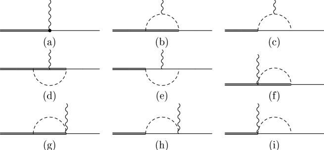
Figure 1: The diagrams contributing to the $\Delta\rightarrow N\gamma$ transition at leading-one-loop order in the SSE formalism [21].

$$G_{1}(q^{2}) = A(\lambda)+\frac{c_{A}M_{N}}{(4\pi F_{\pi})^{2}}\Bigg{[}\Delta_{0}\left(\frac{g_{A}}{3}-\frac{145g_{1}}{81}\right)-\frac{4}{9}\Delta_{0}\int_{0}^{1}\!dx\,\left(5g_{1}(x-3)-9g_{A}(x-1)\right)x\ln{\left(\frac{\tilde{m}}{\lambda}\right)}$$ (16)

$$+\frac{4}{9}\int_{0}^{1}\!dx\,\left(5g_{1}(x-3)I(-x\Delta_{0},\tilde{m})+9g_{A}(x-1)I(x\Delta_{0},\tilde{m})\right)\Bigg{]}+{\cal O}(\epsilon^{4}),$$

$$G_{2}(q^{2}) = B(\lambda)-C_{s}q^{2}+\frac{c_{A}M_{N}^{2}}{(4\pi F_{\pi})^{2}}\Bigg{[}\frac{4}{81}\left(27g_{A}-35g_{1}\right)+\frac{16}{9}(5g_{1}-9g_{A})\int_{0}^{1}\!dx\,x(x-1)\ln{\left(\frac{\tilde{m}}{\lambda}\right)}$$ (17)

$$+\frac{16}{9}\int_{0}^{1}\!dx\,\frac{x^{2}(x-1)}{\tilde{m}^{2}-x^{2}\Delta_{0}^{2}}\Delta_{0}\left(5g_{1}I(-x\Delta_{0},\tilde{m})+9g_{A}I(x\Delta_{0},\tilde{m})\right)\Bigg{]}+{\cal O}(\epsilon^{4}),$$

$$G_{3}(q^{2}) = \frac{8}{9}\frac{c_{A}M_{N}^{2}\Delta_{0}}{(4\pi F_{\pi})^{2}}\int_{0}^{1}\!dx\,\frac{x(2x^{2}-3x+1)}{\Delta_{0}^{2}x^{2}-\tilde{m}^{2}}\left(5g_{1}I(-x\Delta_{0},\tilde{m})+9g_{A}I(x\Delta_{0},\tilde{m})\right)+{\cal O}(\epsilon^{4}).$$ (18)

The corresponding ${\cal O}(\epsilon^{3})$ results in (non-relativistic) SSE for the $N\Delta$-multipole transition form factors $\mathcal{G}_{M}^{*}(q^{2})$, $\mathcal{G}_{E}^{*}(q^{2})$, $\mathcal{G}_{C}^{*}(q^{2})$ are obtained by inserting Eqs.(16-18) into the definitions Eqs.(2-4). In Eqs.(16-18) we have introduced the quantities $\tilde{m}^{2}=m_{\pi}^{2}-q^{2}x(1-x)$ [23] and

$$I(\omega,m_{\pi}) = \left\{\begin{array}[]{l c l}\sqrt{\omega^{2}-m_{\pi}^{2}}\left(\ln{\left(\frac{\omega}{m_{\pi}}+\sqrt{\frac{\omega^{2}}{m_{\pi}^{2}}-1}\right)}-i\pi\right)&&\frac{\omega}{m_{\pi}}>1\\ \sqrt{m_{\pi}^{2}-\omega^{2}}\arccos{\left(-\frac{\omega}{m_{\pi}}\right)}&\,\textnormal{for}&-1\leq\frac{\omega}{m_{\pi}}\leq 1\\ -\sqrt{\omega^{2}-m_{\pi}^{2}}\ln{\left(-\frac{\omega}{m_{\pi}}+\sqrt{\frac{\omega^{2}}{m_{\pi}^{2}}-1}\right)}&&\frac{\omega}{m_{\pi}}<-1.\end{array}\right.$$ (22)

$A(\lambda)$ and $B(\lambda)$ collect all short range physics contributing to $G_{1}(0)$ and $G_{2}(0)$:

$$A(\lambda) = -\frac{1}{2}b_{1}+(2E_{1}^{(r)}(\lambda)-D_{1}^{(r)}(\lambda))\frac{\Delta_{0}}{4M_{N}},$$ (23)

$$B(\lambda) = 2b_{6}-D_{1}^{(r)}(\lambda).$$ (24)

The renormalization scale dependence of the counter terms cancels the one from the loop contributions. We note that the ${\cal O}(\epsilon^{3})$ structure with the coupling constant $E_{1}$ in Eq.(14) arises naturally in SSE. Its infinite part is required for a complete renormalization of the ${\cal O}(\epsilon^{3})$ result, whereas its (scale-dependent) finite part $E_{1}^{(r)}(\lambda)$ cannot be observed independently from the coupling $b_{1}$. For nucleon observables the finite parts of terms like $E_{1}^{(r)}(\lambda)$ are required in order to guarantee the decoupling of the Delta-resonance in the limit $m_{\pi}/\Delta_{0}\rightarrow 0$ (see for example the discussion given in ref.[29]). In $N\Delta$-transition quantities like $G_{1}(q^{2})$ of Eq.(16), the finite coupling $E_{1}^{(r)}(\lambda)$ can be utilized to remove quark-mass independent short distance physics contributions $\sim\Delta_{0}$ from loop diagrams contributing to this form factor. Implementing this constraint one finds

$$E_{1}^{(r)}(\lambda) = -\frac{c_{A}M_{N}^{2}}{324\pi^{2}F_{\pi}^{2}}\left[36g_{A}-139g_{1}+3(35g_{1}-9g_{A})\ln{\left(\frac{2\Delta_{0}}{\lambda}\right)}\right].$$ (25)

We emphasize again that this special choice for $E_{1}^{(r)}(\lambda)$ does not lead to observable consequences in the final result, except for changing the numerical values of the couplings $b_{1}$ and $D_{1}^{(r)}(\lambda)$ by taking away short distance physics $\sim\Delta_{0}$ arising in the loop integrals. Unfortunately, at ${\cal O}(\epsilon^{3})$ in SSE we cannot separate the three independent couplings $b_{1},\,b_{6}$ and $D_{1}^{(r)}(\lambda)$, as we only encounter the two linearly independent combinations $A(\lambda),\,B(\lambda)$ which we fit to experimental input in section 4. We are therefore postponing a discussion of the size of the individual couplings to a future communication [27].

Finally we would like to comment on the constant $C_{s}$ in Eq.(17). To ${\cal O}(\epsilon^{3})$ in non-relativistic SSE all counter terms—i.e. all short distance physics contributions—only appear at $q^{2}=0$, cf. Eqs.(16-18). All radii of the $G_{i}(q^{2})$ form factors therefore arise as pure loop effects from the chiral pion-dynamics at this order. While it is somewhat expected that the dominant parts of these isovector $N\Delta$-transition radii arise from the pion-cloud, it is also known—for example from calculations of the isovector nucleon form factors (see ref.[23])—that short distance contributions in such radii cannot be completely neglected. A short distance contribution to the $r_{2}$-radius of the $N\Delta$-transition form factor $G_{2}(q^{2})$ like $C_{s}$ could, for example, arise from the non-relativistic reduction of the ${\cal O}(\epsilon^{5})$ SSE Lagrangean

$$\mathcal{L}_{N\Delta}^{(5)} \sim C_{s}\bar{\psi}_{\mu}^{i}\gamma_{5}\frac{1}{2}\left(\tau^{i}\left[D^{2},f^{\mu\nu}_{+}\right]\right)D_{\nu}\psi_{N}+h.c..$$ (26)

While this contribution formally is suppressed by two orders in the SSE expansion, we will argue in section 4.2 that the inclusion of such a short distance coupling is crucial for a comparison with phenomenology. We note that the contribution of Eq.(26) to the form factor $G_{2}(q^{2})$ was not considered in ref.[21] and constitutes our main change in terms of formalism compared to those previous results. We note that such radius terms do exist for all form factors, also for the radii of $G_{1}$ or $G_{3}$. We have checked that an inclusion of such terms in $G_{1}$ or $G_{3}$ does not lead to significant changes of the best fit curves, indicating that such terms in $G_{1}$ and $G_{3}$ do behave as small higher order corrections as suggested by the power counting. At the end of section 4.4 we will also discuss the chiral extrapolation of lattice results for the isovector $N\Delta$-transition form factors in the multipole basis at $q^{2}=0$. As the quark-mass dependence of $\mathcal{G}_{M}^{*}(0)$, $\mathcal{G}_{E}^{*}(0)$, $\mathcal{G}_{C}^{*}(0)$ is rather involved (see e.g. the definition equations (2-4)), the specific form of their chiral extrapolation can only be given numerically. However, the leading quark-mass dependence of the $G_{i}(q^{2}),\,i=1\ldots 3$ form factors at $q^{2}=0$ can be given in a closed form:

$$G_{1}(0) = -\frac{1}{2}b_{1}-D_{1}(\lambda)\frac{\Delta_{0}}{4M_{N}}+\frac{ic_{A}g_{A}\Delta_{0}M_{N}}{24\pi F_{\pi}^{2}}$$ (27)

$$+\frac{c_{A}M_{N}m_{\pi}^{2}}{576\Delta_{0}\pi^{2}F_{\pi}^{2}}\left[9g_{A}\left(6-3\pi^{2}+4i\pi-4\ln{\left(\frac{2\Delta_{0}}{m_{\pi}}\right)}\left(1+2i\pi-\ln{\left(\frac{2\Delta_{0}}{m_{\pi}}\right)}\right)\right)\right.$$

$$\left.-5g_{1}\left(10+3\pi^{2}+4\ln{\left(\frac{2\Delta_{0}}{m_{\pi}}\right)}+12\ln^{2}{\left(\frac{2\Delta_{0}}{m_{\pi}}\right)}\right)\right]+\frac{c_{A}(5g_{1}+9g_{A})M_{N}m_{\pi}^{3}}{216\Delta_{0}^{2}\pi F_{\pi}^{2}}+...,$$

$$G_{2}(0) = 2b_{6}-D_{1}(\lambda)-\frac{c_{A}M_{N}^{2}}{162\pi^{2}F_{\pi}^{2}}\left[5g_{1}\left(1+3\ln{\left(\frac{2\Delta_{0}}{\lambda}\right)}\right)+9g_{A}\left(1+3\left(i\pi-\ln{\left(\frac{2\Delta_{0}}{\lambda}\right)}\right)\right)\right]$$ (28)

$$+\frac{c_{A}M_{N}^{2}m_{\pi}^{2}}{144\Delta_{0}^{2}\pi^{2}F_{\pi}^{2}}\left[9g_{A}\left(10-3\pi(\pi-4i)-4\ln{\left(\frac{2\Delta_{0}}{m_{\pi}}\right)}\left(3+2i\pi-\ln{\left(\frac{2\Delta_{0}}{m_{\pi}}\right)}\right)\right)\right.$$

$$\left.-5g_{1}\left(10+\pi^{2}-12\ln{\left(\frac{2\Delta_{0}}{m_{\pi}^{2}}\right)}+4\ln^{2}{\left(\frac{2\Delta_{0}}{m_{\pi}}\right)}\right)\right]+\frac{M_{N}^{2}c_{A}(5g_{1}+9g_{A})m_{\pi}^{3}}{27\Delta_{0}^{3}\pi F_{\pi}^{2}}+...,$$

$$G_{3}(0) = \frac{c_{A}M_{N}^{2}}{648\pi^{2}F_{\pi}^{2}}\left[85g_{1}-9g_{A}(17+6i\pi)+6(9g_{A}-5g_{1})\ln{\left(\frac{2\Delta_{0}}{m_{\pi}}\right)}\right]$$ (29)

$$-\frac{c_{A}(5g_{1}+9g_{A})M_{N}^{2}m_{\pi}}{36\Delta_{0}\pi F_{\pi}^{2}}+\frac{c_{A}M_{N}^{2}m_{\pi}^{2}}{288\Delta_{0}^{2}\pi^{2}F_{\pi}^{2}}\Bigg{[}9g_{A}\Bigg{(}-22+9\pi^{2}-20i\pi+$$

$$4\ln{\left(\frac{2\Delta_{0}}{m_{\pi}}\right)}\left(5+6i\pi-3\ln{\left(\frac{2\Delta_{0}}{m_{\pi}}\right)}\right)\Bigg{)}+5g_{1}\left(22+3\pi^{2}+4\ln{\left(\frac{2\Delta_{0}}{m_{\pi}}\right)}\left(-5+3\ln{\left(\frac{2\Delta_{0}}{m_{\pi}}\right)}\right)\right)\Bigg{]}$$

$$-\frac{c_{A}(5g_{1}+9g_{A})M_{N}^{2}m_{\pi}^{3}}{27\Delta_{0}^{3}\pi F_{\pi}^{2}}+...\,.$$

We observe that the leading quark-mass $m_{q}$ dependence both for $G_{1}(0)$ and for $G_{2}(0)$ is linear in $m_{q}$, whereas the leading non-analytic quark-mass behaviour is proportional to $m_{q}\log m_{q}$, both for the real and for the imaginary parts. On the other hand, $G_{3}(0)$ displays a chiral singularity $\sim\log m_{q}$ near the chiral limit, which will also appear in the Coulomb quadrupole form factor $\mathcal{G}_{C}^{*}(0)$ in section 4.4. Finally, we observe that to ${\cal O}(\epsilon^{3})$ short distance effects arising from the loop integrals could be removed in Eq.(27) from the real part of $G_{1}(0)$ via the choice for $E_{1}^{(r)}(\lambda)$ given in Eq.(25), whereas the real part of $G_{2}(0)$ in Eq.(28) and all imaginary parts are still affected by quark-mass independent short distance physics generated by the loop diagrams of Fig.1. This nuisance can only be remedied at the next order ${\cal O}(\epsilon^{4})$ [27]. In the present ${\cal O}(\epsilon^{3})$ SSE calculation this situation is partly responsible for the rather large fit-values we will obtain for $A(\lambda),\,B(\lambda)$ in the next section.

4 Discussion of the results

4.1 Fit 1: Comparison to previous ${\cal O}(\epsilon^{3})$ SSE results

The strict $\mathcal{O}(\epsilon^{3})$ results of ref.[21] can be obtained from Eqs.(16-18) by setting $C_{s}\equiv 0$. For the numerical values of the input parameters we do not follow that reference but instead we utilize the updated values for the couplings given in table 1. In Fit 1 we determine the two unknown parameters $A(\lambda)$ and $B(\lambda)$ by inserting Eqs.(16)-(18) into Eqs.(2)-(4) and fit
a) to the experimental data for $\left|\mathcal{G}_{M}^{*Ash}(Q^{2})\right|$ shown in figure 2 for momentum transfers of $Q^{2}<0.2$ GeV² and simultaneously
b) to the experimental value for EMR$(0)$ of ref.[2] utilizing Eq.(7).
The resulting values of this Fit 1 are given in table 2 for a regularization scale of $\lambda=1$ GeV.

Parameter	$g_{A}$	$c_{A}$	$g_{1}$	$M_{N}$ [GeV]	$M_{\Delta}$ [GeV]	$m_{\pi}$ [GeV]	$F_{\pi}$ [GeV]
Value	1.26	1.5	2.8	0.939	1.210	0.14	0.0924

Table 1: The input parameters for our calculation. The nucleon properties $g_{A}$ and $M_{N}$ are taken from [1]. For the definition of the mass of $\Delta$(1232) we are utilizing the T-matrix definition of [1], leading to a (real part) mass of $1210$ MeV. The coupling $g_{1}$ has recently been determined in [31], whereas the value for $c_{A}$ is derived in Appendix B.

Parameter	$A$(1GeV)	$B$(1GeV)	$C_{s}$ [GeV-2]
Fit I	10.5	15.4	0 (fixed)
Fit II	10.5	15.4	-17.0

Table 2: The values for the unknown parameters obtained by fitting our results to the experimental data for $\left|\mathcal{G}_{M}^{*Ash}(Q^{2}<0.2GeV^{2})\right|$ and EMR$(0)$ at a regularization scale of $\lambda=1$ GeV. In Fit I we set $C_{s}=0$. We note that the values for A and B do not change significantly between Fit 1 and Fit 2.

The dashed curve in Figure 2 shows, that this procedure leads to a satisfying description of $\left|\mathcal{G}_{M}^{*Ash}(Q^{2})\right|$ up to $Q^{2}\approx 0.2$ GeV². We note that the dotted curve also shown in that figure is the parametrization of the MAID result [32], which takes into account the fact that this form factor is falling faster than the dipole by inserting an extra exponential function:

$$\left|\mathcal{G}_{M}^{*Ash}(Q^{2})\right| = \frac{3}{\left(1+\frac{Q^{2}}{0.71\textnormal{GeV}^{2}}\right)^{2}}\exp{\left(-0.21\frac{Q^{2}}{\textnormal{GeV}^{2}}\right)}.$$ (30)

However, while we obtain a reasonable $Q^{2}$-dependence for the magnetic $N\Delta$-transition form factor up to $Q^{2}\approx 0.2$ GeV², we only get the right value of EMR($Q^{2}$) at the photon point $Q^{2}=0$, while the $Q^{2}$-dependence of this ratio is far off the experimental data. This can be seen from the dashed curve in Fig.3. A similarly non-satisfying picture results for the $Q^{2}$-dependence of the CMR-ratio, see Fig.4. We have analysed the reason for these early breakdowns in $Q^{2}$ of the ${\cal O}(\epsilon^{3})$ SSE calculation of ref.[21]. According to our new analysis presented here these small ratios are very sensitive to the exact form of the $G_{2}(Q^{2})$ form factor. As it can be seen from the dotted curve of $G_{2}(Q^{2})$ in Fig.5, in Fit 1 the momentum transfer dependence of the real part of $G_{2}$ has an (unphysical) turning point already at rather low $Q^{2}$. It begins to rise again above $Q^{2}\approx 0.05$ GeV². This “unnatural” behaviour is an indication that important physics is not included in the SSE-calculation at the order we are working. Our analysis shows that it is this “unphysical” behaviour of the $G_{2}(q^{2})$ form factor which is responsible for the poor results of the $Q^{2}$-dependence in EMR$(Q^{2})$ and CMR$(Q^{2})$ in Fit 1. In the next section we will present a remedy for this breakdown. In conclusion we must say that for state-of-the art coupling constants as given in table 1 the non-relativistic ${\cal O}(\epsilon^{3})$ SSE calculation for the (small) electric and coulomb $N\Delta$-quadrupole transition form factors of ref.[21] is only valid up for $Q^{2}<0.05$ GeV², while the (much larger) magnetic $N\Delta$-transition form factor is described well with the results of ref.[21] over a larger range in $Q^{2}$.

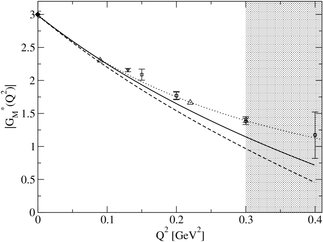
Figure 2: The absolute value of the magnetic $N\Delta$-transition form factor $\mathcal{G}_{M}^{*Ash}(Q^{2})$ in the convention of Eq.(5) to ${\cal O}(\epsilon^{3})$ in non-relativistic SSE. Solid line: Fit 2. Dashed line: Fit 1. Dotted line: MAID parametrization [32]. Experimental data from [2] (diamond), [3] (triangle up), [34] (triangle down), [4] (square) and [5] (circle).

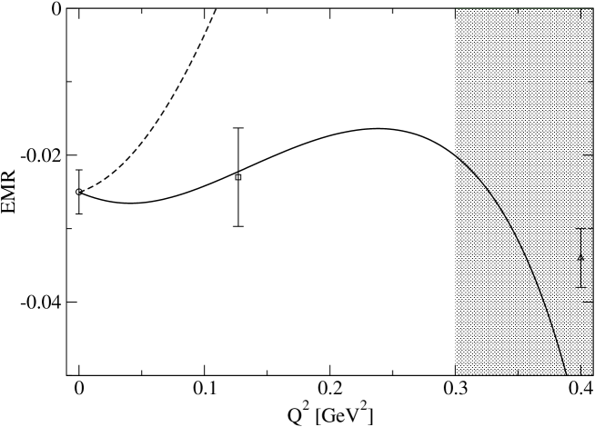
Figure 3: EMR$(Q^{2})$ to ${\cal O}(\epsilon^{3})$ in non-relativistic SSE. Dashed line: Fit 1. Solid line: Fit 2. Experimental data at the real photon point from MAMI [2], at $Q^{2}=0.127$ GeV² from OOPS [8] and at $Q^{2}=0.4$ GeV² from CLAS [7].

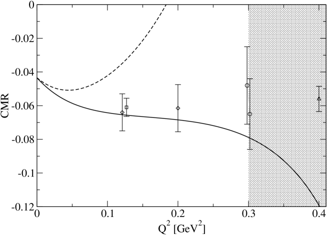
Figure 4: CMR$(Q^{2})$ to ${\cal O}(\epsilon^{3})$ in non-relativistic SSE. Dashed line: Fit 1. Solid line: Fit 2. The data-points shown are from refs. [9] (diamonds), [6] (circles) and [7] (triangle).

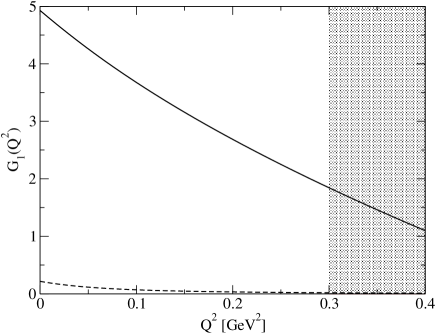
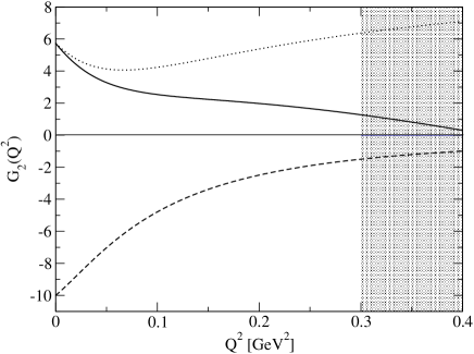
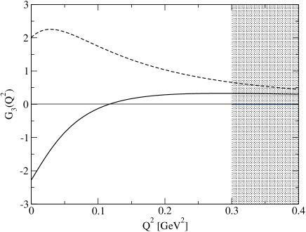
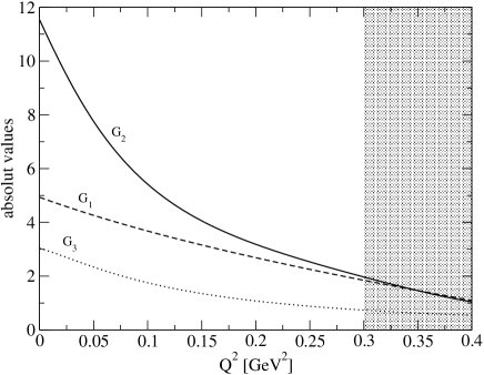
Figure 5: The form factors $G_{1}$, $G_{2}$ and $G_{3}$ defined in Eq.(1). Solid lines show the real parts, dashed lines imaginary parts. The dotted line in the plot for $G_{2}(Q^{2})$ arises in Fit 1, whereas the solid line corresponds to Fit 2. The absolute value of $G_{2}(Q^{2})$ shown in the panel on the lower right corresponds to Fit 2.

4.2 Fit 2: Revised ${\cal O}(\epsilon^{3})$ SSE analysis

The early breakdown of the ${\cal O}(\epsilon^{3})$ SSE calculation of ref.[21] discussed in the previous section can be overcome by introducing the parameter $C_{s}$ in Eq.(17). As discussed in section 3 such a term formally arises from higher order couplings in the ${\cal O}(\epsilon^{5})$ Lagrangean like the one displayed in Eq.(26). Physically, this term amounts to a (small) short distance correction in the radius of the form factor $G_{2}(Q^{2})$, which in Fit 1 is given solely by pion-loop contributions. One may wonder, why such a contribution, which formally is of much higher order in the perturbative chiral calculation, suddenly should play such a prominent role. However, we have to point out that the (rather small) electric $\mathcal{G}_{E}^{*}(Q^{2})$ form factor is very sensitive to the $N\Delta$-transition form factor $G_{2}(Q^{2})$. The size of this quadrupole form factor is at the percent level of the dominant magnetic $\mathcal{G}_{M}^{*}(Q^{2})$ transition form factor—small changes in $G_{2}(Q^{2})$ are therefore disproportionally magnified when looking at EMR$(Q^{2})$. In the following we will explicitly include the radius term in Fit 2, which now has three unknown parameters $A(\lambda),B(\lambda)$ and $C_{s}$. Utilizing the same input parameters as in Fit 1 (see table 1) we insert Eqs.(16)-(18) into Eqs.(2)-(4) and fit again
a) to the same experimental data for $\left|\mathcal{G}_{M}^{*Ash}(Q^{2})\right|$ shown in Fig.2 at momentum transfers of $Q^{2}<0.2$ GeV² and simultaneously
b) to the experimental value for EMR$(0)$ reported in ref.[2] utilizing Eq.(7).
We note that neither in Fit 1 of the previous section nor in the new Fit 2 we have fit to the CMR$(q^{2})$ data of Fig.4. In both fits the resulting curves are a prediction. The results for the three parameters of this new Fit 2 are given in table 2. First we notice that the central values for the parameters $A(1$ GeV$),B(1$ GeV$)$ have not changed significantly. While the numerical value for the new parameter $C_{s}$ is quite large, it actually only amounts to a small correction of $0.21$ fm in the $r_{2}$ radius, in agreement with the expectation from the chiral counting:

$$r_{2,\textnormal{Re}}:\,1.57\,\textnormal{fm (Fit 1)} \rightarrow 1.78\,\textnormal{fm (Fit 2)}.$$ (31)

This small correction in the radius of the $G_{2}(Q^{2})$ form factor leads to a much more physical behaviour in the real part of $G_{2}$ for $Q^{2}<0.4$ GeV², as can clearly be seen from the solid curve in Fig.5. The resulting changes in the momentum-dependence of EMR and CMR as shown in the solid curves of Figs.3, 4 are quite astonishing. The small change in the radius of $G_{2}$ has lead to agreement with experimental data both for EMR and CMR up to a four-momentum transfer squared of $Q^{2}\approx 0.3$ GeV². We note again that none of the experimental data points at finite $Q^{2}$ in EMR or CMR have been used as input for the determination of the fit-parameters. The significant change of the Quadrupole form factors caused by the inclusion of the radius term which is formally of higher order proves that it underestimated by naive power counting. At the same time the resulting good accordance with phenomenology shows, that this term includes relevant physics into our calculation. These two observations constitute our justification for the inclusion of the coupling $C_{S}$. For completeness we also note that the resulting absolute value of $\mathcal{G}_{M}^{*}(Q^{2})$ of Fit 2 is now also in decent agreement with the experimental data up to $Q^{2}\approx 0.2\ldots 0.3$ GeV². We therefore conclude that in Fit 2, after the radius correction in $G_{2}(Q^{2})$ has been inserted, it is now the insufficient momentum-dependence of $\mathcal{G}_{M}^{*}(Q^{2})$ above $Q^{2}\approx 0.25$ GeV² that sets the limit in $Q^{2}$ for the new non-relativistic ${\cal O}(\epsilon^{3})$ SSE result of Fit 2 presented here. We indicate this limitation by the gray-shaded bands in Figs.2-4 and will explore this point further in section 4.3

In table 3 we present the results of Fit 2 for all six $N\Delta$-transition form factors discussed in this work, both at $Q^{2}=0$ and for their (complex) radii, defined as:

$$G_{i}(Q^{2}) = \textnormal{Re}[G_{i}(0)]\left[1-\frac{1}{6}r_{i,\textnormal{Re}}^{2}Q^{2}+...\right]+i\,\textnormal{Im}[G_{i}(0)]\left[1-\frac{1}{6}r_{i,\textnormal{Im}}^{2}Q^{2}+...\right].$$ (32)

	$\textnormal{Re}[G_{i}(0)]$	$r_{i,\textnormal{Re}}^{2}$ [fm2]	$\textnormal{Im}[G_{i}(0)]$	$r_{i,\textnormal{Im}}^{2}$ [fm2]	$\left|G_{i}(0)\right|$	$r_{i,\textnormal{Abs}}^{2}$ [fm2]
$G_{1}$	4.95	0.679	0.216	3.20	4.96	0.678
$G_{2}$	5.85	3.15	-10.0	1.28	11.6	1.73
$G_{3}$	-2.28	3.39	2.01	-2.26	3.04	0.907
$\mathcal{G}_{M}^{*}$	2.98	0.627	-0.377	1.36	3.00	0.630
$\mathcal{G}_{E}^{*}$	0.0441	-0.836	-0.249	0.422	0.253	0.388
$\mathcal{G}_{C}^{*}$	1.10	-0.729	-1.68	1.90	2.01	1.10

Table 3: The values at $Q^{2}=0$ and the radii of the two sets of form factors used in this work obtained in Fit 2.

It is interesting to note that the real parts of the radii of both the electric and the coulomb $N\Delta$-transition form factors are negative! This can also be observed in Fig.6: The quadrupole $N\Delta$-transition form factors definitely do not behave like dipoles in the low $Q^{2}$-region, they look different both from the Sachs form factors of the nucleon and from the common parametrization for $\mathcal{G}_{M}^{*}(Q^{2})$ of Eq.(30).

Table 3 and Fig.6 constitute the central results of our analysis. They make clear, that the non-trivial $Q^{2}$-dependence of EMR$(Q^{2})$ and CMR$(Q^{2})$ observed in Figs. 3, 4 arises from the quadrupole transition form factors, which should therefore be studied independently of $\mathcal{G}_{M}^{*}(Q^{2})$. Finally we want to comment on the size of the short distance contributions “$sd$” parametrized via $A(1$ GeV$),\,B(1$ GeV$)$ versus the long distance contributions from the pion-cloud “$pc$”. Despite the large values for these combinations of LECs (see Eqs.(23,24)), the $N\Delta$-transition form factors are not completely dominated by short distance physics —clear signatures of chiral dynamics are visible. At a scale of $\lambda=1$ GeV one obtains (at the photon point):

$$\textnormal{Re}[\mathcal{G}_{M}^{*}(0)]|_{\lambda=1\,\textnormal{GeV}} = \left.-1.06\right|_{pc}+\left.4.04\right|_{sd},$$ (33)

$$\textnormal{Re}[\mathcal{G}_{E}^{*}(0)]|_{\lambda=1\,\textnormal{GeV}} = \left.0.155\right|_{pc}-\left.0.110\right|_{sd},$$ (34)

$$\textnormal{Re}[\mathcal{G}_{C}^{*}(0)]|_{\lambda=1\,\textnormal{GeV}} = \left.1.47\right|_{pc}-\left.0.365\right|_{sd}.$$ (35)

We note that such a separation into short and long range physics is obviously scale-dependent. However, at a much lower regularization scale of $\lambda=600$ MeV we have checked that one arrives at the same pattern. Analyzing Eqs.(33-35) we conclude that the magnetic $N\Delta$-transition is dominated by short distance physics. Its strength is ${\it reduced}$ by $\approx 40\%$ due to pion-cloud effects in the magnetic $N\Delta$-transition. This result is very similar to the situation in the isovector magnetic moment of the nucleon (see the discussion in ref.[29]), both in sign and in magnitude!
While the pion-cloud and the short distance physics are of the same magnitude but of opposite sign for the very small electric quadrupole transition moment, the coulomb quadrupole moment in our non-relativistic ${\cal O}(\epsilon^{3})$ SSE analysis is dominated by the chiral dynamics of the pion-cloud. We note that the small resulting value for CMR$(Q^{2})$ is of purely kinematical origin (see Eq.(7)), whereas the electric quadrupole form factor in the Jones-Scadron conventions used in this work is intrinsically small relative to the magnetic M1 transition form factor. We will report in a future communication [27] whether this pattern Eqs.(33-35) will hold also at next-to-leading one-loop order (i.e. ${\cal O}(\epsilon^{4})$) in SSE, where we also hope to project out individual values for three leading $\gamma N\Delta$-couplings $b_{1},\,b_{6}$ and $D_{1}^{(r)}(\lambda)$ [27]. Before we discuss the quark-mass dependence of the form factors we first want to comment on the range of $Q^{2}$ in which the non-relativistic ${\cal O}(\epsilon^{3})$ SSE calculation seems applicable.

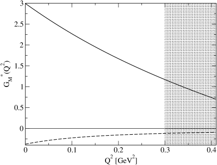
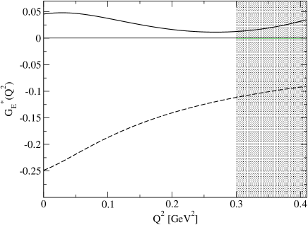
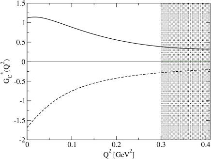
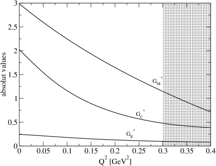
Figure 6: $\mathcal{O}(\epsilon^{3})$ SSE results of Fit 2 for the $N\Delta$-transition form factors in the multipole-basis. Solid lines: Real parts. Dashed lines: Imaginary parts.

4.3 Range of applicability of the non-relativistic ${\cal O}(\epsilon^{3})$ SSE calculation

In non-relativistic ${\cal O}(\epsilon^{3})$ SSE calculations the isovector Sachs form factors of the nucleon agree well with dispersion-theoretical results up to a four-momentum transfer of $Q^{2}\approx 0.3$ GeV² (see e.g. the discussion in ref.[33]). On the other hand, it is known that covariant ChEFT calculations of baryon form factors usually do not find enough curvature in the $Q^{2}$-dependence of such form factors beyond the radius term linear in $Q^{2}$ (e.g. see ref.[38]), due to a different organisation of the (perturbative) ChEFT series. We suspect that this is also the reason why the $Q^{2}$-dependence of EMR and CMR reported recently in the covariant ChEFT calculation of ref.[26] is markedly different from the one presented here.
In our non-relativistic ${\cal O}(\epsilon^{3})$ SSE analysis the limiting factor—as far as the $Q^{2}$-dependence is concerned—seems to be the deviation between the result of Fit 2 for $\mathcal{G}_{M}^{*}(Q^{2})$ (solid curve in Fig.2) compared to the data (parametrized by the dotted curve). In order to demonstrate this we present EMR$(Q^{2})$ and CMR$(Q^{2})$ again in Figures 7, 8, now with $\mathcal{G}_{M}^{*}(Q^{2})$ not given by our result of Fit 2 but with the exponential parametrization of Eq.(30). One can clearly observe that in both figures the agreement with the experimental results now extends to even larger values of $Q^{2}$, giving us confidence that the here calculated results for the electric and coulomb $N\Delta$ quadrupole-transition form factors—which are the quantities where the impact of chiral dynamics shows up most visibly (see the discussion in section 4.2)—have captured the relevant physics up to a momentum transfer $Q^{2}\approx 0.3$ GeV², similar to the situation for the isovector Sachs form factors of the nucleon in non-relativistic ${\cal O}(\epsilon^{3})$ SSE [33]. We also note that the slope of the SSE result for CMR at $Q^{2}<0.1$ GeV² is highly dominated by $\pi N$ intermediate states (originating from diagram (c) in Fig.1). The plateau in this ratio at higher momentum transfer is due to a balance between this loop effect and short range physics, with the larger $r_{2}$ radius of Fit 2 (see Eq.31) again being essential. We also observe in Fig.8 that the DMT model of ref.[22] shows the same feature at low $Q^{2}$ as our SSE calculation. It is also interesting to note that the turnover in the $Q^{2}$-dependence of EMR near $Q^{2}\approx 0.25$ GeV² in Fig.7 may not signal the breakdown of our approach at this (already quite large) momentum transfer, but could indicate a real structure effect connecting the OOPS and the CLAS results for EMR$(Q^{2})$. In order to decide this issue clearly the next-to-leading one-loop correction to our results has to be calculated [27]. Finally, we note again explicitly that the resulting dashed curves in Fig.7 and Fig.8 have not been refit to the data points at finite $Q^{2}$, despite their “perfect“ agreement with the shown data.

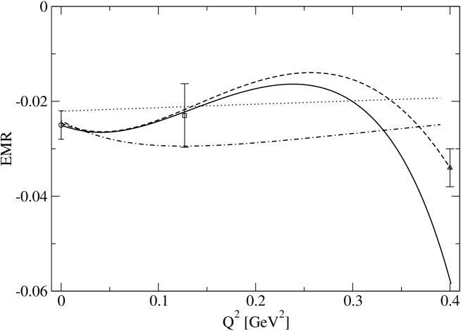
Figure 7: EMR$(Q^{2})$ at small momentum transfer. Solid line: ${\cal O}(\epsilon^{3})$ SSE result of Fit 2. Dashed line: EMR$(Q^{2})$ with parametrized $\mathcal{G}_{M}^{*}$ of Eq.(30) and the ${\cal O}(\epsilon^{3})$ SSE result of Fit 2 for $\mathcal{G}_{E}^{*}$. The dotted and dashed-dotted lines are results of the MAID2003 and DMT models [22]. For explanations on the data-points shown see Fig.3.

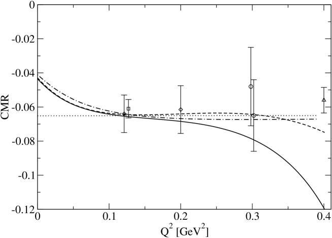
Figure 8: CMR$(Q^{2})$ at small momentum transfer. Solid line: ${\cal O}(\epsilon^{3})$ SSE result of Fit 2. Dashed line: CMR$(Q^{2})$ with parametrized $\mathcal{G}_{M}^{*}$ of Eq.(30) and the ${\cal O}(\epsilon^{3})$ SSE result of Fit 2 for $\mathcal{G}_{C}^{*}$. The dotted and dashed-dotted lines are results of the MAID2003 and DMT models [22]. For explanations on the data-points shown see Fig.4.

4.4 Chiral extrapolation of the $N\Delta$-transition form factors to ${\cal O}(\epsilon^{3})$ in non-relativistic SSE

An upcoming task in the description of the nucleon to $\Delta$ transition in chiral effective field theory is the study of the quark-mass dependence of these form factors, extrapolating the recent lattice results of refs.[39],[41] to the physical point. Figure 9 shows —as a first step on this way — the pion-mass dependence of the $N\Delta$-transition form factors in the Jones-Scadron basis of Eqs.(2-4) according to non-relativistic $\mathcal{O}(\epsilon^{3})$ SSE. We note that we did not refit any of the parameters of table 2 to produce the extrapolation functions shown—all parameters have been fixed from experimental observables at the physical point as described in sections 4.1, 4.2. Both the real and the imaginary parts of the three $N\Delta$-transition form factors develop a quark-mass $m_{q}$-dependence, which has been translated into a dependence on the mass of the pion $m_{\pi}$ via the GOR-relation [30]

$$m_{\pi}^{2} = 2\,B_{0}\,m_{q}+\mathcal{O}(m_{q}^{2}),$$ (36)

consistent with the order at which we are working. $B_{0}$ denotes the magnitude of the chiral condensate. The imaginary parts of all three form factors shown in Fig.9 vanish for $m_{\pi}>\Delta_{0}$, since the $\Delta$(1232) resonance would become a stable particle at this large pion-mass. It is interesting to observe, that the quark-mass dependence of the magnetic dipole $N\Delta$-transition moment $\mu_{N\Delta}=\textnormal{Re}\left[\mathcal{G}_{M}^{*}(0)\right]$ qualitatively shows the same behaviour as the isovector magnetic moment $\mu_{N}^{v}$ of the nucleon, studied e.g. in ref.[29]. Like its analogue $\mu_{N}^{v}$, at the physical point ($m_{\pi}=140$ MeV) $\mu_{N\Delta}$ is substantially reduced from its chiral limit value by $\approx$ 25 percent, dropping further rather quickly in size for increasing quark masses. On the other hand, the quark-mass dependence of both the electric and the coulomb quadrupole $N\Delta$-transition moments $Q_{E}^{N\Delta}=\textnormal{Re}\left[\mathcal{G}_{E}^{*}(0)\right]$ and $Q_{C}^{N\Delta}=\textnormal{Re}\left[\mathcal{G}_{C}^{*}(0)\right]$ is rather unexpected: As can be seen from Fig.9 $Q_{E}^{N\Delta}$ even changes its sign around $m_{\pi}\approx 100$ MeV, before approaching a negative value in the chiral limit. It will be very interesting to see how the location of this zero-crossing might be affected by corrections at next-to-leading one-loop order $\mathcal{O}(\epsilon^{4})$ in SSE [27]. In the case of $Q_{C}^{N\Delta}$ one can observe the effect of $G_{3}(0)$ of Eq.(29), leading to a logarithmic divergence of the coulomb quadrupole transition strength in the chiral limit. Curiously, our non-relativistic ${\cal O}(\epsilon^{3})$ SSE calculation indicates that $Q_{C}^{N\Delta}$ is near a local maximum for physical quark-masses. Given the dominance of chiral $\pi N$-physics in this form factor (see the discussion in section 4.3), it would be extremely exciting if such a behaviour could be observed in a lattice QCD simulation. Unfortunately, present state-of-the-art lattice simulations for $N\Delta$-transition form factors take place for $m_{\pi}>370$ MeV [39], which is outside the region of applicability of this non-relativistic leading-one-loop SSE calculation, as indicated by the grey bands in Figs. 9, 10. We hope to extend the range in $m_{\pi}$ of the chiral extrapolation functions for the $N\Delta$-transition considerably when going to next order in the calculation [27]. We also note that the leading-one-loop covariant calculation in the $\delta$-expansion scheme presented in ref.[26]—which contains the same diagrams as our non-relativistic ${\cal O}(\epsilon^{3})$ SSE calculation, see Fig.1—seems to be also stable at pion masses larger than $m_{\pi}\approx 200$ MeV, presumably due to the additional $m_{\pi}/M_{N}$ terms present in a covariant approach. However, the stability of the chiral extrapolation functions of both schemes should be tested further by going to next-to-leading one-loop order.

Furthermore, we want to note that there is no need to consider the rather complex structures of EMR or CMR when comparing to lattice QCD results. The intricacies—i.e. the sought after signatures of chiral dynamics—can be studied in a much cleaner fashion when directly comparing ChEFT results to lattice QCD simulations of the $N\Delta$-transition form factors (e.g in the Jones-Scadron basis), see Fig. 9. Nevertheless, for completeness, in Fig. 10 we also show our results for the chiral extrapolation functions of the real parts of EMR(0) and CMR(0) defined as

$$emr = -\frac{\textnormal{Re}[\mathcal{G}_{E}^{*}(0)]}{\textnormal{Re}[\mathcal{G}_{M}^{*}(0)]},$$ (37)

$$cmr = -\frac{M_{\Delta}^{2}-M_{N}^{2}}{4M_{\Delta}^{2}}\frac{\textnormal{Re}[\mathcal{G}_{C}^{*}(0)]}{\textnormal{Re}[\mathcal{G}_{M}^{*}(0)]}\;.$$ (38)

The discussed sign-change in $Q_{E}^{N\Delta}$ is visible in Fig. 10 in emr, while the exciting chiral structures of $Q_{C}^{N\Delta}$ dominate cmr for pion masses $m_{\pi}<200$ MeV. As already mentioned, available lattice data of these quantities in refs.[39, 41] are unfortunately at too large pion-masses to be relevant for the chiral extrapolation functions presented here. However—independent of this (present) limitation of our ChEFT results with respect to small pion-masses—we have to note one important general caveat for (future) comparisons of ChEFT results to lattice QCD simulations of $N\Delta$ form factors: In Figs.9,10 we discuss the chiral extrapolation of the three $N\Delta$-transition moments at $Q^{2}=0$, while lattice QCD results are usually obtained at finite values of momentum transfer. In order to correct for this, one often attempts to connect the lattice results of finite $Q^{2}$ to the real photon point by performing global dipole fits, with the dipole mass as a free (quark-mass dependent) parameter fit from lattice data. While such a procedure may lead to promising results, for example, in the case of the form factors of the nucleon (see the discussion in ref.[33])—and also seems to be applicable to the (monotonously falling) magnetic dipole $N\Delta$-transition form factor $\mathcal{G}_{M}^{*}(Q^{2})$— it should not be applied to the study of the sought after electric and coulomb quadrupole $N\Delta$-transition form factors, due to the non-trivial momentum dependence in these form factors for $Q^{2}<0.15$ GeV². This can be clearly concluded from Fig. 6 and from the negative values of (the real parts of) their radii in table 3. Global dipole fits connecting lattice QCD results from large $Q^{2}$ across the region $Q^{2}<0.15$ GeV² to the photon point at $Q^{2}=0$ would just ”wash-out” all the interesting chiral physics which dominates the $N\Delta$ quadrupole transition moments $Q_{E}^{N\Delta},\,Q_{C}^{N\Delta}$ at the physical point! If one wants to study these objects in lattice QCD one has to perform simulations at such small values of momentum transfer that one can directly compare with the ChEFT results for the three $N\Delta$ transition form factors $\mathcal{G}_{M}^{*}(Q^{2},m_{\pi}^{2})$, $\mathcal{G}_{E}^{*}(Q^{2},m_{\pi}^{2})$, $\mathcal{G}_{C}^{*}(Q^{2},m_{\pi}^{2})$ in the $(Q^{2},m_{\pi}^{2})$-plane, and then utilize a function for the momentum-dependence down to $Q^{2}=0$ which is consistent with the turning-points generated by chiral $\pi N$-dynamics. Figure 11 shows the non-relativistic ${\cal O}(\epsilon^{3})$ SSE result of such a three dimensional function for $\mathcal{G}_{M}^{*}(Q^{2},m_{\pi}^{2})$, further quantitative studies regarding these chiral extrapolation surfaces are relegated to future work [27].

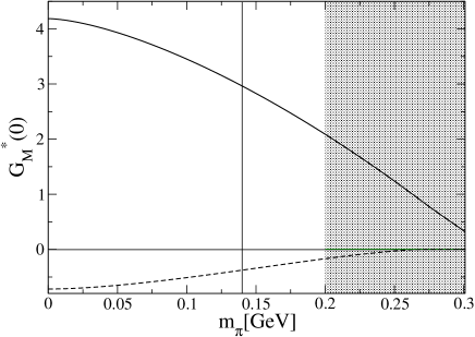
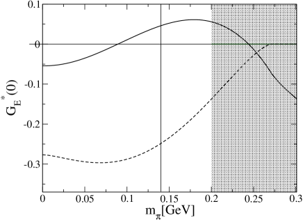
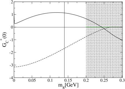
Figure 9: The quark mass dependence of the $N\Delta$-transition form factors in the Jones-Scadron basis according to non-relativistic $\mathcal{O}(\epsilon^{3})$ SSE. Solid lines denote the real parts, dashed lines the imaginary parts. We note that we have assumed here that all masses appearing in the definitions of the Jones-Scadron multipole form factors are taken at their values at the physical point, in order to display only the intrinsic quark-mass dependence of the transition form factors.

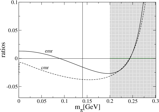
Figure 10: $m_{\pi}$-dependence of the real parts of EMR and CMR at $Q^{2}=0$ according to non-relativistic $\mathcal{O}(\epsilon^{3})$ SSE. We note that we have assumed here that all masses appearing in the definitions of the Jones-Scadron multipole form factors are taken at their values at the physical point, in order to display only the intrinsic quark-mass dependence of the transition form factors.

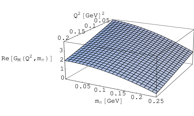
Figure 11: $Q^{2}$ and $m_{\pi}$ dependence of the magnetic dipole $N\Delta$-transition form factor in non-relativistic ${\cal O}(\epsilon^{3})$ SSE.

5 Conclusions and Outlook

The pertinent results of our analysis can be summarized as follows:

1. We have analysed and updated the ${\cal O}(\epsilon^{3})$ SSE calculation of the isovector $N\Delta$-transition current of ref.[21] in terms of the magnetic dipole, electric quadrupole and coulomb quadrupole transition form factors in Fit 1. It was found that the momentum-range of reliability of these results is extremely small, $Q^{2}<0.05$ GeV².

2. We have identified an “unnatural” momentum dependence in the $N\Delta$-transition form factor $G_{2}(Q^{2})$ as the reason for the early breakdown of the results of Fit 1. In section 4.2 we have demonstrated that the inclusion of a (higher order) counter term, which changes the radius of $G_{2}(Q^{2})$ by 0.21 fm, is sufficient to correct the momentum transfer behaviour in this form factor. We have checked that similar correction terms in the radii of $G_{1}$ and $G_{3}$ are not significant. The physical origin of the short distance contribution to the radius of $G_{2}$ parametrized in coupling $C_{S}$ is not understood at present. The results of Fit 2 which includes this correction then showed a consistent behaviour in all three form factors up to a momentum transfer (squared) of $Q^{2}=0.25\ldots 0.3$ GeV².

3. Connecting our results for the transition form factors with ratios of measured pion-electroproduction multipoles via Eqs.(6,7) we have obtained a remarkable agreement between the results of Fit 2 and experiment up to a momentum transfer (squared) of $Q^{2}=0.25\ldots 0.3$ GeV² both for EMR($Q^{2}$) and CMR($Q^{2}$).

4. Long distance pion physics was found to be present in all three $N\Delta$-transition form factors. It showed up most prominent in the momentum dependence of the quadrupole form factors for $Q^{2}<0.15$ GeV², leading to momentum dependencies which cannot be described via a (modified) dipole ansatz anymore. According to our analysis, in pion-electroproduction experiments this feature should show up most clearly in a rise of CMR for $Q^{2}<<0.1$ GeV². It is expected that this rise can be observed within the accuracy of state-of-the art pion-electroproduction experiments in the near future [42]. Another observable signal of chiral dynamics in the $N\Delta$-transition could be a minimum in EMR near $Q^{2}=0.05$ GeV² and a maximum near $Q^{2}=0.25$ GeV². Unlike the case of CMR, however, it is not clear whether these effects can be identified unambiguously given the size of current experimental error bars in EMR$(Q^{2})$.

5. We have studied the chiral extrapolation of the three $N\Delta$-transition form factors at $Q^{2}=0$. We found that the magnetic $N\Delta$ dipole transition moment decreases monotonously with the quark-mass, displaying a qualitatively similar behaviour as the isovector magnetic moment of the nucleon. On the other hand, the quark-mass dependencies of the quadrupole $N\Delta$-transition moments were found to display rapid changes for pion masses below 200 MeV. While the electric quadrupole transition moment $Q_{E}^{N\Delta}$ in our analysis even changes its sign near $m_{\pi}=0.1$ GeV before approaching a negative chiral limit value, we found that the coulomb quadrupole transition moment $Q_{C}^{N\Delta}$ has a local maximum near the physical pion mass, while it diverges in the chiral limit. State-of-the-art lattice simulations cannot yet reach such small pion masses to test these predictions. On the other hand, our non-relativistic ${\cal O}(\epsilon^{3})$ SSE analysis presented here was found to break down for $m_{\pi}>0.2$ GeV.

6. We also want to point out that lattice studies of the quadrupole $N\Delta$ transition form factors cannot be analyzed via a simple dipole ansatz to obtain information about the moments at $Q^{2}=0$ due to the turning-points and structures in the $Q^{2}$ dependence of these form factors at $Q^{2}<0.1$ GeV².

In the future we are planning to calculate the quark-mass dependence of the $N\Delta$-transition form factors at ${\cal O}(\epsilon^{4})$ in order to extend the range of applicability of these results for chiral extrapolations and to test the stability of the structure effects discussed in this work [27]. In conclusion we can say that we have indeed detected interesting signatures of chiral dynamics in the $N\Delta$-transition, both for the momentum and for the quark-mass dependence. In particular we hope that the electric- and coulomb quadrupole $N\Delta$ transition moments will get tested with higher precision both on the lattice and in electron scattering experiments in order to verify the signatures of chiral dynamics discussed in this work.

Appendix A Integrals

The result of the non-relativistic $\mathcal{O}(\epsilon^{3})$ SSE calculation written in terms of standard loop integrals reads:

$$G_{1}(q^{2}) = \frac{2c_{A}M_{N}}{F_{\pi}^{2}}\int_{0}^{1}\!dx\bigg{[}g_{A}(x-1)J_{2}^{\prime}(x\Delta_{0},\tilde{m}^{2})-\frac{5}{3}g_{1}\left(1-\frac{d-3}{d-1}x\right)J_{2}^{\prime}(-x\Delta_{0},\tilde{m}^{2})\bigg{]}$$ (39)

$$-\frac{1}{2}b_{1}+(2E_{1}-D_{1})\frac{\Delta_{0}}{4M_{N}}$$

$$G_{2}(q^{2}) = \frac{8c_{A}M_{N}^{2}}{F_{\pi}^{2}}\int_{0}^{1}\!dx\bigg{[}g_{A}x(x-1)J_{1}^{\prime}(x\Delta_{0},\tilde{m}^{2})-\frac{5}{3}g_{1}x(x-1)\frac{d-3}{d-1}J_{1}^{\prime}(-x\Delta_{0},\tilde{m}^{2})\bigg{]}$$ (40)

$$+2b_{6}-D_{1}$$

$$G_{3}(q^{2}) = \frac{4c_{A}M_{N}^{2}\Delta_{0}}{F_{\pi}^{2}}\int_{0}^{1}\!dx\bigg{[}g_{A}x(x-1)(1-2x)J_{0}^{\prime}(x\Delta_{0},\tilde{m}^{2})-$$ (41)

$$\frac{5}{3}g_{1}x(x-1)(2x-1)\frac{d-3}{d-1}J_{0}^{\prime}(-x\Delta_{0},\tilde{m}^{2})\bigg{]}.$$

The basic loop integrals in d-dimensional regularization are defined as:

$$\frac{1}{i}\int\frac{d^{d}l}{(2\pi)^{d}}\frac{1}{m_{\pi}^{2}-l^{2}} = \Delta_{\pi}\,=\,2m_{\pi}^{2}\left(L+\frac{1}{16\pi^{2}}\ln{\frac{m_{\pi}}{\lambda}}\right)$$ (42)

$$\frac{1}{i}\int\frac{d^{d}l}{(2\pi)^{d}}\frac{1}{(v\cdot l-\omega)(m_{\pi}^{2}-l^{2})} = J_{0}(\omega,m_{\pi}^{2}).$$ (43)

The analytic expression for the one-nucleon-one-pion loop integral is:

$$J_{0}(\omega,m_{\pi}^{2}) = -4L\omega+\frac{\omega}{8\pi^{2}}\left(1-2\ln{\frac{m_{\pi}}{\lambda}}\right)$$ (47)

$$-\frac{1}{4\pi^{2}}\left\{\begin{array}[]{l c l}\sqrt{\omega^{2}-m_{\pi}^{2}}\left(\ln{\left(\frac{\omega}{m_{\pi}}+\sqrt{\frac{\omega^{2}}{m_{\pi}^{2}}-1}\right)}-i\pi\right)&&\frac{\omega}{m_{\pi}}>1\\ \sqrt{m_{\pi}^{2}-\omega^{2}}\arccos{\left(-\frac{\omega}{m_{\pi}}\right)}&\,\textnormal{for}&-1\leq\frac{\omega}{m_{\pi}}\leq 1\\ -\sqrt{\omega^{2}-m_{\pi}^{2}}\ln{\left(-\frac{\omega}{m_{\pi}}+\sqrt{\frac{\omega^{2}}{m_{\pi}^{2}}-1}\right)}&&\frac{\omega}{m_{\pi}}<-1\end{array}\right.$$

$$J_{0}^{\prime}(\omega,m_{\pi}^{2}) = -\frac{\partial}{\partial m_{\pi}^{2}}J_{0}(\omega,m_{\pi}^{2}),$$ (48)

$$J_{1}^{\prime}(\omega,m_{\pi}^{2}) = -\frac{\partial}{\partial m_{\pi}^{2}}\left(\omega J_{0}(\omega,m_{\pi})+\Delta_{\pi}\right),$$ (49)

$$J_{2}^{\prime}(\omega,m_{\pi}^{2}) = -\frac{1}{d-1}\frac{\partial}{\partial m_{\pi}^{2}}\left[(m_{\pi}^{2}-\omega^{2})J_{0}(\omega,m_{\pi})-\omega\Delta_{\pi}\right].$$ (50)

The divergences at $d=4$ parametrized via dimensional regularization are collected in the function $L$ in the $\overline{\textnormal{MS}}$-scheme:

$$L = \frac{\lambda^{d-4}}{16\pi^{2}}\left[\frac{1}{d-4}+\frac{1}{2}\left(\gamma_{E}-1-\ln{4\pi}\right)\right].$$ (51)

Appendix B The coupling constant $c_{A}$

We determine the strength of the $N\Delta$ axial coupling constant $c_{A}$ from the strong decay width of the $\Delta(1232)$ resonance at tree level. In the rest frame of the $\Delta$ this width reads:

$$\Gamma_{\Delta\rightarrow N\pi} = \frac{c_{A}^{2}}{6\pi F_{\pi}^{2}}\left(E_{\pi}^{2}-m_{\pi}^{2}\right)^{\frac{3}{2}}\cdot\frac{M_{\Delta}+M_{N}-E_{\pi}}{2M_{\Delta}},$$ (52)

where the $\pi N\Delta$-vertex has been taken from Eq.(12) and the associated pion energy function reads:

$$E_{\pi} = \frac{M_{\Delta}^{2}-M_{N}^{2}+m_{\pi}^{2}}{2M_{\Delta}}.$$ (53)

For the numerical determination of $c_{A}$ we use the parameters $M_{\Delta}$, $M_{N}$, $m_{\pi}$ and $F_{\pi}$ from table 1, a width of $\Gamma_{\Delta\rightarrow N\pi}=100$ MeV [1] and arrive at the result $c_{A}=1.5$.

References

- [1] S. Eidelman et al. (Particle Data Group), Phys. Lett. B592:1 (2004).
- [2] R. Beck et al., Phys. Rev. C61:035204 (2000).
- [3] S. Stein et al., Phys. Rev. D12:1884 (1975).
- [4] K. Bätzner et al., Phys. Lett. B39:575-578 (1972).
- [5] W. Bartel et al., Phys. Lett. B28:148-151 (1968).
- [6] R. Siddle et al., Nucl. Phys. B35:93-119 (1971) and K. Baetzner et al., Nucl. Phys. B76:1-14 (1974).
- [7] K. Joo et al. (CLAS Collaboration), Phys. Rev. Lett. 88:122001 (2002).
- [8] N.F. Sparveris et al. (OOPS Collaboration), Phys. Rev. Lett. 94:022003 (2005).
- [9] Th. Pospischil et al., Phys. Rev. Lett. 86:2959-2962 (2001) and D. Elsner et al., preprint [nucl-ex/0507014].
- [10] A.M. Bernstein, Eur. Phys. J. A17, 349 (2003).
- [11] A. Wirzba and W. Weise, Phys. Lett. B188:6 (1987).
- [12] T. Sato and T.S.H. Lee, Phys. Rev. C63:055201 (2001) and T. Sato and T.S.H. Lee, Phys. Rev. C54:2660-2684 (1996).
- [13] A.J. Buchmann, in Proceedings of Baryons 98, Ed.: B.Metsch, World Scientific, Singapore (1999). [hep-ph/9909385].
- [14] D.-H. Lu, A.W. Thomas, A.G. Williams, Phys. Rev. C55:3108-3114 (1997).
- [15] A. Silva et al., Nucl. Phys. A675:637-657 (2000).
- [16] J. Gasser, M.E. Sainio, A. Svarc, Nucl. Phys. B307:779 (1988).
- [17] E. Jenkins, A.V. Manohar, Phys. Lett. B255:558-562 (1991).
- [18] V.Bernard, N.Kaiser, J.Kambor, U.-G. Meißner, Nucl. Phys. B388:315-345 (1992).
- [19] M.N. Butler, M.J. Savage, R.P. Springer, Phys. Rev. D49:3459-3465 (1994).
- [20] T.R. Hemmert, B.R. Holstein and J. Kambor,. J. Phys. G24:1831-1859 (1998).
- [21] G.C. Gellas, T.R. Hemmert, C.N. Ktorides and G.I. Poulis, Phys. Rev. D60:054022 (1999).
-
[22]
S.S. Kamalov, et al., Phys. Rev. Lett. 83:4494 (1999) and Phys. Rev. C 64:032201 (2001).
D. Drechsel, O. Hanstein, S.S. Kamalov and L. Tiator, Nucl. Phys. A645:145 (1999).
http://www.kph.uni-mainz.de/MAID - [23] V. Bernard, H.W. Fearing, T.R. Hemmert and U.-G. Meißner, Nucl. Phys. A635:121-145 (1998), Erratum-ibid. A642:563-563 (1998).
- [24] H.F. Jones and M.D. Scadron, Annals Phys.81:1-14 (1973).
- [25] W.W. Ash, et al., Phys. Lett. B24, 165 (1967).
- [26] V. Pascalutsa and M. Vanderhaeghen, preprint [hep-ph/0508060].
- [27] T.A. Gail et al., in preparation.
- [28] V. Bernard, N. Kaiser and U.-G. Meißner, Int. J. Mod. Phys. E4:193-346 (1995).
- [29] T.R. Hemmert and W. Weise, Eur. Phys. J. A15:487-504 (2002).
- [30] M. Gell-Mann, R.J. Oakes and B. Renner, Phys. Rev. 175:2195-2199 (1968).
- [31] M. Göckeler et al, Proceedings of Science LAT2005:349 (2005)[hep-lat/0510061] and A.Ali Khan et al., preprint [hep-lat/0603028]..
- [32] S.S. Kamalov, et al., Phys. Rev. C64:032201 (2001).
- [33] M. Göckeler et al., Phys. Rev. D71:034508 (2005).
- [34] L. Tiator, D. Drechsel, S.S. Kamalov and S.N. Yang, Eur. Phys. J. A17:357-363 (2003).
- [35] R.P. Hildebrandt, H.W. Griesshammer, T.R. Hemmert and B. Pasquini, Eur. Phys. J. A20:293-315 (2004).
- [36] J. Bijnens and F. Cornet, Nucl. Phys. B296:557 (1988).
- [37] J.F. Donoghue, B.R. Holstein and Y.C. Lin, Phys. Rev. D37:2423 (1988).
- [38] B. Kubis and U.-G. Meißner, Nucl. Phys. A679:698-734 (2001).
- [39] C. Alexandrou, et al., Phys. Rev. Lett. 94:021601 (2005).
- [40] T.R. Hemmert, M. Procura and W. Weise, Phys. Rev. D68:075009 (2003).
- [41] C. Alexandrou et al. (Lattice Hadron Collaboration), J. Phys. Conf. Ser. 16:174-178 (2005).
- [42] A.M. Bernstein, private communication.