Universal scaling of the elliptic flow data at RHIC

Abstract

Recent PHOBOS measurements of the excitation function for the pseudo-rapidity dependence of elliptic flow in Au+Au collisions at RHIC, have posed a significant theoretical challenge. Here we show that these differential measurements, as well as the RHIC measurements on transverse momentum satisfy a universal scaling relation predicted by the Buda-Lund model, based on exact solutions of perfect fluid hydrodynamics. We also show that recently found transverse kinetic energy scaling of the elliptic flow is a special case of this universal scaling.

.1 Introduction

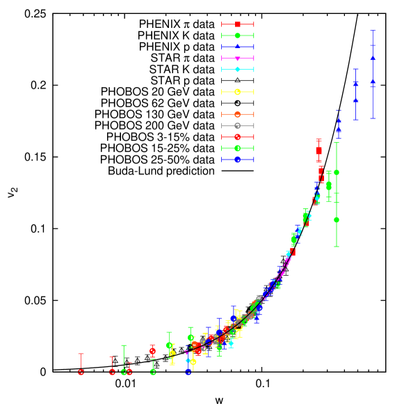
One of the unexpected results from experiments at the Relativistic Heavy Ion Collider (RHIC) is the relatively strong second harmonic moment of the transverse momentum distribution, referred to as the elliptic flow. Measurements of the elliptic flow by the PHENIX, PHOBOS and STAR collaborations (see refs. Back:2004zg ; Back:2004mh ; Adler:2003kt ; Adams:2004bi ; Adler:2001nb ; Sorensen:2003wi ) reveal rich details in terms of its dependence on particle type, transverse ($p_{t}$) and longitudinal momentum ($\eta$) variables, and on the centrality and the bombarding energy of the collision. In the soft transverse momentum region ($p_{t}\lesssim 2$ GeV/c) measurements at mid-rapidity are found to be well described by hydrodynamical models Adcox:2004mh ; Adams:2005dq . By contrast, differential measurement of the pseudo-rapidity dependence of elliptic flow and its excitation function have resisted several attempts at a description in terms of hydrodynamical models (but see their description by the SPHERIO model Grassi:2005pm ; Andrade:2007aa or the approximate descriptions in refs. Nonaka:2007nn ; Bleibel:2006xx ). Here we show that these data are consistent with theoretical, analytic predictions that are based on perfect fluid hydrodynamics: Fig. 1 demonstrates that the investigated PHOBOS, PHENIX and STAR data Back:2004zg ; Back:2004mh ; Adler:2003kt ; Adams:2004bi follow the theoretically predicted scaling law.

.2 Perfect fluid hydro picture

Perfect fluid hydrodynamics is based on local conservation of entropy $\sigma$ and four-momentum tensor $T^{\nu\mu}$,

$$\partial_{\mu}(\sigma u^{\mu}) = 0,$$ (1)

$$\partial_{\nu}T^{\mu\nu} = 0,$$ (2)

where $u^{\mu}$ stands for the four-velocity of the matter. The fluid is perfect if the four-momentum tensor is diagonal in the local rest frame,

$$T^{\mu\nu}=(\epsilon+p)u^{\mu}u^{\nu}-pg^{\mu\nu}.$$ (3)

Here $\epsilon$ stands for the local energy density and $p$ for the pressure. These equations are closed by the equation of state, which gives the relationship between $\epsilon$, $p$ and $\sigma$, typically $\epsilon=\kappa p$ is assumed, where $\kappa$ is either a constant Csorgo:2003ry or an arbitrary temperature dependent function Csorgo:2001xm that uses a non-relativistic approximation. Note also, that a bag constant can also be introduced, and the $\epsilon-B=\kappa(p+B)$ equation of state can be used Csorgo:2003rt ; Nagy:2007xn .

We focus here on the analytic approach in exploring the consequences of the presence of such perfect fluids in high energy heavy ion experiments in Au+Au collisions at RHIC. Such a nonrelativistic exact analytic solution was published in ref. Csorgo:2001xm , while relativistic solutions were published in refs. Csorgo:2003rt ; Sinyukov:2004am ; Nagy:2007xn . For a detailed discussion on new exact relativistic solutions, see ref. Nagy:2007xn .

A tool, that is based on the above listed exact, dynamical hydro solutions, is the Buda-Lund hydro model of refs.  Csorgo:1995bi ; Csanad:2003qa . This hydro model is successful in describing experimental data on single particle spectra and two-particle correlations  Csanad:2003sz ; Csanad:2004cj . The model is defined with the help of its emission function; to take into account the effects of long-lived resonances, it utilizes the core-halo model Csorgo:1994in .

The elliptic flow is an experimentally measurable observable and is defined as the azimuthal anisotropy or second fourier-coefficient of the one-particle momentum distribution $N_{1}(p)$. The definition of the flow coefficients is:

$$v_{n}=\frac{\int_{0}^{2\pi}N_{1}(p)\cos(n\varphi)d\varphi}{\int_{0}^{2\pi}N_{1}(p)d\varphi},$$ (4)

where $\varphi$ is the azimuthal angle of the momentum. This formula returns the elliptic flow $v_{2}$ for $n=2$.

.3 Universal scaling of the elliptic flow in the Buda-Lund model

The result for the elliptic flow, that comes directly from a perfect hydro solution is the following simple scaling law Csorgo:2001xm ; Csanad:2003qa

$$v_{2}=\frac{I_{1}(w)}{I_{0}(w)},$$ (5)

where $I_{n}(z)$ stands for the modified Bessel function of the second kind, $I_{n}(z)=(1/\pi)\int_{0}^{\pi}\exp(n\cos(\theta))\cos(n\theta)d\theta$.

Note that this prediction was derived first in 2001 in a non-relativistic perfect hydrodynamical solution, see eq. (25) of ref. Csorgo:2001xm . In 2003, it has been extended to the relativistic kinematic domain in ref. Csanad:2003qa . Ref. Csanad:2003qa considered a relativistic parameterization that included a multitude of known relativistic solutions, such as the Hwa-Bjorken solution Hwa:1974gn ; Bjorken:1982qr or other accelerating and Hubble-type of solutions Csorgo:2003rt ; Sinyukov:2004am ; Nagy:2007xn , and interpolated among these.

The subject of our current investigation is the testing of this scaling law against recent experimental data, but let us first discuss this scaling law.

In the Buda-Lund hydro model, elliptic flow depends only on momentum space anisotropy, but it does not depend on the coordinate space anisotropy. This feature of the Buda-Lund model Csanad:2008af is different from azimuthally sensitive Blast-wave models Retiere:2003kf , where $v_{2}$ depends also on the coordinate space distribution.

In section .4, we explain the universal scaling variable $w$ in eq. (5) and show, how $w$ can be determined from measurements. In section .5, we shall subject this relationship to an experimental test also.

.4 Variable of the universal scaling law of $v_{2}$

Looking at eq. (5), one sees that the Buda-Lund hydro model predicts Csorgo:2001xm a universal scaling: every $v_{2}$ measurement is predicted to fall on the same scaling curve $I_{1}/I_{0}$ when plotted against the scaling variable $w$. This means, that $v_{2}$ depends on any physical parameter (transverse or longitudinal momentum, mass, center of mass energy, collision centrality, type of the colliding nucleus etc.) only through the scaling variable $w$. This scaling variable is defined by:

$$w=\frac{E_{K}}{T_{*}}\varepsilon$$ (6)

Here $E_{K}$ is a relativistic generalization of the transverse kinetic energy, defined as

$$E_{K}=\frac{p_{t}^{2}}{2\overline{m}_{t}},$$ (7)

with

$$\overline{m}_{t}=m_{t}\cosh\left(\frac{y}{1+\Delta\eta\frac{m_{t}}{T_{0}}}\right),$$ (8)

$y$ being the rapidity, $\Delta\eta$ the longitudinal expansion of the source, $T_{0}$ the central temperature at the freeze-out and $m_{t}=\sqrt{p_{t}^{2}+m^{2}}$ the transverse mass. We note, that at mid-rapidity and for a leading order approximation, $E_{K}\approx m_{t}-m$, which also explains recent development on scaling properties of $v_{2}$ by the PHENIX experiment at midrapidity Adare:2006ti ; Afanasiev:2007tv . We furthermore note, that parameter $\Delta\eta$ has recently been dynamically related Nagy:2007xn to the acceleration parameter of new exact solutions of relativistic hydrodynamics, where the accelerationless limit corresponds to a Bjorken type, flat rapidity distribution and the $\Delta\eta\rightarrow\infty$ limit.

The scaling variable $w$ also depends on the parameter $T_{*}$, which is the effective, rapidity and transverse mass dependent slope of the azimuthally averaged single particle spectra, and on the final momentum space eccentricity parameter, $\varepsilon$. These can be defined Csorgo:2001xm ; Csanad:2003qa by the transverse mass and rapidity dependent slope parameters of the single particle spectra in the impact parameter (subscript _x) and out of the reaction plane (subscript _y) directions, $T_{x}$ and $T_{y}$,

$$\frac{1}{T_{*}} = \frac{1}{2}\left(\frac{1}{T_{x}}+\frac{1}{T_{y}}\right),$$ (9)

$$\varepsilon = \frac{T_{x}-T_{y}}{T_{x}+T_{y}}.$$ (10)

which are thus observable quantities. Note also, that $\varepsilon$ can also be interpreted as a measure of integrated $v_{2}$, and thus setting the absolute scale of $v_{2}$.

Figure 1: Elliptic flow data of previous plots versus variable $w$ is shown: Data points show the predicted Csanad:2003qa universal scaling. Small scaling violations at large $w$ values correspond to $v_{2}(p_{t})$ data for $p_{t}>2$ GeV. Note, that the error of $w$ was not plotted on this plot, but it can be determined from data analysis, and it is on the order of 5-20%.

In the Buda-Lund hydro model Csorgo:2001xm ; Csanad:2003qa , the rapidity and the transverse mass dependence of the slope parameters is given as

$$T_{x} = T_{0}+\overline{m}_{t}\dot{X}^{2}\frac{T_{0}}{T_{0}+\overline{m}_{t}a^{2}},$$ (11)

$$T_{y} = T_{0}+\overline{m}_{t}\dot{Y}^{2}\frac{T_{0}}{T_{0}+\overline{m}_{t}a^{2}}.$$ (12)

Here $a^{2}=\langle\frac{\Delta T}{T}\rangle$ measures the transverse temperature inhomogeneity of the particle emitting source in the transverse direction at the mean freeze-out time.

We note, that each of the kinetic energy term, the effective temperature $T_{*}$ and the eccentricity $\varepsilon$ are transverse mass and rapidity dependent factors. However, for $\overline{m}_{t}a^{2}\gg T_{0}$, $T_{x}$ and $T_{y}$, hence $\varepsilon$ and $T_{*}$ become independent of transverse mass and rapidity. This saturation of the slope parameters happens only if the temperature is inhomogeneous, ie $a^{2}>0$.

The above structure of $w$, the variable of the universal scaling function of elliptic flow suggests that the transverse momentum, rapidity, particle type, centrality, colliding energy, and colliding system dependence of the elliptic flow is only apparent in perfect fluid hydrodynamics: a data collapsing behavior sets in and a universal scaling curve emerges, which coincides with the ratio of the first and zeroth order modified Bessel functions Csorgo:2001xm ; Csanad:2003qa , when $v_{2}$ is plotted against the scaling variable $w$.

Interesting is furthermore, that the Buda-Lund hydro model also predicts the following universal scaling laws and relationships for higher order flows Csanad:2003qa : $v_{2n}=I_{n}(w)/I_{0}(w)$ and $v_{2n+1}=0$. This is to be tested in a later, more detailed analysis.

.5 Comparison to experimental data

We emphasize first, that the scaling variable $w$ is expressed in eq. (6) in terms of factors, that are in principle measurable (however, these factors are not yet determined directly from experimental data). The elliptic flow $v_{2}$ is also directly measurable. Hence the universal scaling prediction, eq. (5) can in principle be subjected to a direct experimental test. Given the fact that such measurements were not yet published in the literature, we perform an indirect testing of the prediction, by determining the relevant parameters of the scaling variable $w$ from an analysis of the transverse momentum and rapidity dependence of the elliptic flow in Au+Au collisions at RHIC.

Transverse momentum dependent elliptic flow data at mid-rapidity can be compared to the Buda-Lund universal scaling prediction of 2001 and 2003 of the Buda-Lund model directly, as it was done in e.g. ref. Csanad:2003qa .

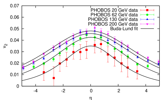
Eq. (5) depends, for a given centrality class, on rapidity $y$ and transverse mass $m_{t}$. When comparing our result to $v_{2}(\eta)$ data of the PHOBOS Collaboration, we have performed a saddle point integration in the transverse momentum variable and performed a change of variables to the pseudo-rapidity $\eta=0.5\log(\frac{|p|+p_{z}}{|p|-p_{z}})$, similarly to ref. Kharzeev:2001gp . This way, we have evaluated the single-particle invariant spectra in terms of the variables $\eta$ and $\phi$, and calculated $v_{2}(\eta)$ from this distribution, a procedure corresponding to the PHOBOS measurement described in ref. Back:2004zg .

Scaling implies data collapsing behavior, and also is reflected in a difficulty in extracting the precise values of these parameters from elliptic flow measurements: due to the data collapsing behavior, some combinations of these fit parameters become relevant, other combinations become irrelevant quantities, that cannot be determined from measurements. This is illustrated in Fig. 1, where we compare the universal scaling law of eq. (5) with elliptic flow measurements at RHIC. This figure shows an excellent agreement between data and prediction. We may note the small scaling violations at largest $w$ values, that correspond to elliptic flow data taken in the transverse momentum region of $p_{t}>2$ GeV.

The observed scaling itself shows, that only a few relevant combinations of $T_{0}$, $a^{2}$, $\dot{X}^{2}$, $\dot{Y}^{2}$ determine the transverse momentum dependence of the $v_{2}$ measurements. Hence from these measurements it is not possible to reconstruct all these four source parameters uniquely. We have chosen the following to eq. (5) approximative formulas to describe the scaling of the elliptic flow:

$$w(\eta) = \frac{2A}{\cosh(B\eta)}\textrm{, and}$$ (13)

$$w(p_{t}) = A^{\prime}\frac{p_{t}^{2}}{4m_{t}}\left(1+B^{\prime}(m_{t}-m)+C^{\prime}(m_{t}-m)^{2}\right),$$ (14)

and for small values of $w$ eq. (5) simplifies to $v_{2}\approx w/2$. The coefficients are as follows:

$$A = \left.\frac{E_{K}}{2T_{*}}\varepsilon\right|_{m_{t}=\langle m_{t}\rangle,y=0}$$ (15)

$$B = \left.\left(1+\Delta\eta\frac{m_{t}}{T_{0}}\right)^{-1}\right|_{m_{t}=\langle m_{t}\rangle,y=0}$$ (16)

$$A^{\prime} = \left.\frac{2\varepsilon}{T_{*}}\right|_{m_{t}=m,y=0}$$ (17)

$$B^{\prime} = \left.-\frac{1}{m}\frac{T_{0}}{T_{0}+ma^{2}}\left(1-2\frac{T_{0}}{T_{*}}\right)\right|_{m_{t}=m,y=0}$$ (18)

$$C^{\prime} = \frac{1}{m}\left(\frac{T_{0}}{T_{0}+ma^{2}}\right)^{5}\left.\frac{1}{T_{x}^{2}T_{y}^{2}}\right|_{m_{t}=m,y=0}\times$$

$$\times \left[({\dot{X}}^{2}+a^{2}+{\dot{Y}}^{2})(T_{0}+ma^{2})^{3}+\right.$$

$$+ m{\dot{X}}^{2}{\dot{Y}}^{2}\left(m^{2}({\dot{X}}^{2}{\dot{Y}}^{2}+a^{2}({\dot{X}}^{2}+{\dot{Y}}^{2}))\right)$$

$$- \left.3m{\dot{X}}^{2}{\dot{Y}}^{2}T_{0}(T_{0}+ma^{2})\right].$$

From this simple picture we had to deviate a little bit in case of proton $v_{2}(p_{t})$ data, here only one parameter could have been used to find a valid Minuit James:1975dr minimum, so we fixed B’ there.

For the case of kaons and protons, only $A^{\prime}$ and $B^{\prime}$ were significant, while pion data were so detailed, that $C^{\prime}$ could have been determined, too. Thus we used it only when fitting pion $v_{2}(p_{t})$ .

For the analysis of the PHOBOS $v_{2}(\eta)$ measurements at RHIC, we have excluded points with large rapidity from lower center of mass energies $v_{2}(\eta)$ fits ($\eta>4$ for 19.6 GeV, $\eta>4.5$ for 62.4 GeV). Points with large transverse momentum ($p_{t}>2.0$ GeV) were excluded from PHENIX and STAR $v_{2}(p_{t})$ fits. These values give a hint at the boundaries of the validity of the model.

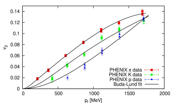
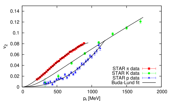
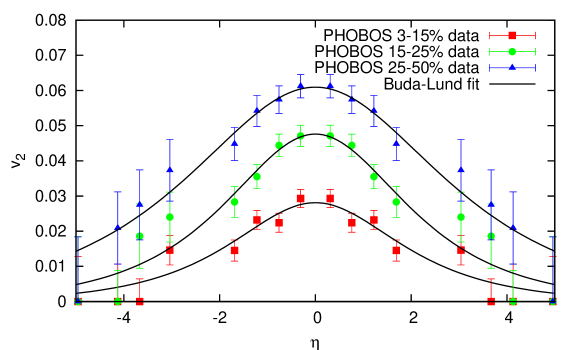
Fits to PHOBOS Back:2004zg ; Back:2004mh , PHENIX Adler:2003kt and STAR Adams:2004bi data are shown in Figs. 2 and 3. The values of the parameters and the quality of the fits are summarized in Table 1.

Using the fit parameters in Table 1 and eqs. (13-14), we have determined the universal scaling variable $w$ from these PHENIX, PHOBOS and STAR data.

Using these $w$ values we have plotted the data against $w$ in Fig. 1. Note that on this plot $w$ itself has an error, as it is a reconstructed variable based on eqs. (15-.5) and the values and the errors of the parameters as given in Table 1. Standard error propagation has been applied and we have obtained that the relative error of $w$ changes between 5-50%, and is above 20% only for $v_{2}(\eta)$ points with large $\eta$ and pion $v_{2}(p_{t})$ points with large $p_{t}$. As Fig. 1 is best seen when the values of $w$ are plotted on a logarithmic scale, these relative errors of $w$ do not change the qualitative conclusion. Comparing with the solid black line in Fig. 1 we observe, that elliptic flow data from various STAR, PHENIX and PHOBOS measurements at RHIC follow the universal scaling curve, predicted by the ellipsoidally symmetric Buda-Lund model in 2004.

$v_{2}(\eta)$	20GeV		62GeV		130GeV		200GeV
A	0.035$\pm$	0.004	0.043$\pm$	0.001	0.046$\pm$	0.001	0.048$\pm$	0.001
B	0.53$\pm$	0.1	0.41$\pm$	0.01	0.34$\pm$	0.01	0.33$\pm$	0.01
$\chi^{2}/$NDF	1.7/11		9.3/13		17/15		18/15
CL	91%		74%		30%		28%
$v_{2}(\eta)$	3-15%		15-25%		25-50%
A	0.028$\pm$	0.002	0.048$\pm$	0.002	0.061$\pm$	0.002
B	0.64$\pm$	0.08	0.60$\pm$	0.06	0.43$\pm$	0.04
$\chi^{2}/$NDF	12/13		8/13		4/13
CL	51%		84%		96%

$v_{2}(p_{t})$	$\pi$		K		p
A’ [$10^{-4}$/MeV]	5.4$\pm$	0.1	6.4$\pm$	0.3	3.0$\pm$	0.1
B’ [$10^{-4}$/MeV]	16$\pm$	1	-0.2$\pm$	0.4	25, fixed
C’ [$10^{-6}$/MeV2]	-1.5$\pm$	0.1	—		—
$\chi^{2}/$NDF	96/27		17/5		27/26
CL	1$\times 10^{-7}$%		0.5%		40%
$v_{2}(p_{t})$	$\pi$		K		p
A’ [$10^{-4}$/MeV]	7.8$\pm$	0.2	7.4$\pm$	0.3	5.8$\pm$	0.1
B’ [$10^{-4}$/MeV]	1.4$\pm$	0.6	-1.3$\pm$	0.4	1.6, fixed
C’ [$10^{-7}$/MeV2]	-1.6$\pm$	0.3	—		—
$\chi^{2}/$NDF	21/10		13/9		17/7
CL	2%		15%		2%

Table 1: Values of the parameters and the quality of the fits for collision energy dependent PHOBOS $v_{2}(\eta)$ data Back:2004zg is shown in the top table, the same for centrality dependent PHOBOS $v_{2}(\eta)$ data Back:2004mh in the second table. The third shows STAR Adams:2004bi , the fourth PHENIX Adler:2003kt $v_{2}(p_{t})$ data results.

Figure 2: PHENIX Adler:2003kt and STAR Adams:2004bi data on elliptic flow, $v_{2}$, plotted versus $p_{t}$ and fitted with Buda-Lund model.

Figure 3: PHOBOS Back:2004zg ; Back:2004mh data on elliptic flow, $v_{2}$, plotted versus $\eta$ and fitted with Buda-Lund model.

I Further scaling properties

From the Taylor expansion of the Bessel functions for the realistic $w\ll 1$ case one finds

$$v_{2}\approx\frac{w}{2}.$$ (20)

One can also see, that for small momenta,

$$E_{K}=\frac{p_{t}^{2}}{2m_{t}}\approx m_{t}-m.$$ (21)

Thus a leading order calculation, at mid-rapidity, from eq. (14) one gets

$$v_{2}\approx\frac{A^{\prime}}{4}(m_{t}-m).$$ (22)

This derivation indicates, that the PHENIX discovery Adare:2006ti ; Afanasiev:2007tv of the universal scaling of the elliptic flow in terms of $m_{t}-m$ at mid-rapidity is a consequence, a special case of the more general universal scaling law of eq. 5, predicted by the Buda-Lund model.

Furthermore, PHENIX found Adare:2006ti ; Afanasiev:2007tv , that $v_{2}/n_{q}$ scales in terms of $(m_{t}-m)/n_{q}$ for several types of particles ($\pi$, K, K${}^{0}_{s}$, p, $\Lambda$, $\Xi$, deuteron, $\Phi$). This indicates that the perfect fluid motion scales on the quark level, and the Buda-Lund model scaling prediction for higher order flows, $v_{2n}=I_{n}(w)/I_{0}(w)$ (see ref. Csanad:2003qa ) should also be applied on the quark level.

I.1 Conclusions

We have shown that the excitation function of the transverse momentum and pseudorapidity dependence of the elliptic flow in Au+Au collisions is well described with the formulas that are predicted by the Buda-Lund type of hydrodynamical calculations Csorgo:2001xm ; Csanad:2003qa . We have provided a positive test for the validity of the perfect fluid picture of soft particle production in Au+Au collisions at RHIC up to  1-1.5 GeV and up to a pseudorapidity of $\eta_{\textrm{beam}}-0.5$.

We have also shown that the PHENIX discovery Adare:2006ti ; Afanasiev:2007tv of a scaling behavior of $v_{2}$ vs. $m_{t}-m$ is a special case of the more general, rapidity dependent universal scaling law of the Buda-Lund type of perfect fluid hydrodynamical solutions.

The universal scaling of PHOBOS $v_{2}(\eta)$ and PHENIX and STAR $v_{2}(p_{t})$ , expressed by eq. (5) and illustrated by Fig. 1 provides a successful quantitative as well as qualitative test for the appearance of a perfect fluid in Au+Au collisions at various colliding energies at RHIC.

We have furthermore shown, that since PHENIX found Adare:2006ti ; Afanasiev:2007tv , that $v_{2}/n_{q}$ scales in terms of $(m_{t}-m)/n_{q}$ for several types of particles, the Buda-Lund model scaling prediction for higher order flows, $v_{2n}=I_{n}(w)/I_{0}(w)$ (see ref. Csanad:2003qa ) should also be applied on the quark level.