Microscopic analysis of shape-phase transitions in even-even $N\sim 90$ rotating nuclei

Abstract

We study in cranked Nilsson plus random phase approximation shape transitions in fast rotating nuclei undergoing backbending, more specifically ¹⁵⁶Dy and ¹⁶²Yb. We found that a backbending in ¹⁵⁶Dy is correlated with the disappearance of the collective, positive signature $\gamma$-vibrational mode in the rotating frame, and, a shape transition (axial$\rightarrow$ nonaxial) is accompanied with a large acquiring of the $\gamma$ deformation. We show that such a shape transition can be considered as a phase transition of the first order. In ¹⁶²Yb the quasiparticle alignment dominates in the backbending and the shape transition (axial$\rightarrow$ nonaxial) is accompanied with a smooth transition from zero to nonzero values of the $\gamma$ deformation. We extend the classical Landau theory for rotating nuclei and show that the backbending in ${}^{162}Yb$ is identified with the second order phase transition. A description of spectral and decay properties of the yrast states and low-lying excitations demonstrates a good agreement between our results and experimental data.

I Introduction

Backbending is a paradigm of structural changes in a nucleus under rotation. A sudden increase of a nuclear moment of inertia in yrast rotational band at some critical angular momentum or rotational frequency, discovered few decades ago Jon , continues to attract a considerable attention. There is a general persuasion that this phenomenon is a result of the rotational alignment of angular momenta of a nucleon pair occupying a high-j intruder orbital near the Fermi surface (see textbooks RS ; Rag and references therein). However, it is understood just recently, that this point of view may obscure different mechanisms if applied to nuclei with relatively small axial deformation at zero spin. In particular, Regan et al Re proposed that the backbending observed in a number Cd, Pd and Ru nuclei can be interpreted as a change from vibrational to rotational structure. In our preliminary report JK1 , we proposed to consider the backbending in $N\sim 90$ as a result of the transition from axially symmetric to nonaxial shape due to a disappearance of a collective $\gamma$-vibrational mode in the rotating frame.

The analogy of the backbending phenomenon with a behaviour of superconductors in magnetic field, noticed in Ref.mot, , is rising a desire to apply Landau theory of phase transitions Lan to nuclei. We recall that Landau’s theory deals with second order phase transitions, when different macroscopic phases become indistinguishable at the transition point. Whether it takes place for rotating nuclei is an open question. Nuclei are finite systems and phase transitions should be washed out by quantum fluctuations. Nevertheless, long ago Thouless t22 proposed to distinguish two kinds of ”phase transitions” even for nuclei. Such phase transitions may be connected with shape transitions, for example, from spherical to deformed or axially deformed to nonaxially deformed shapes. This idea was put ahead in the analysis of shape transitions in hot rotating nuclei Al . In this case the statistical treatment of the finite-temperature mean field description had provided a justification for an application of the Landau theory for nuclei. Within this approach, a simple rules for different shape-phase transitions were found as a function of angular momentum and temperature.

Recently, quantum phase transitions, that occur at zero temperature as a function of some nonthermal control parameter, attract a considerable attention in various branches of many-body physics, starting from low-dimensional systems Sad to atomic nuclei and molecules Zam . Until the present a major activity in the study of shape-phase transitions for nuclei in the ground state at zero temperature is carried out within the interacting boson model (IBM) (see, for example, Refs.Jo02, ; cej, and references therein). The model naturally incorporates different symmetry limits associated with specific nuclear properties nat . While the IBM can be easily extended to a thermodynamical limit $N\rightarrow\infty$, which is well suitable for the study of phase transitions, the analysis is rather oversimplified. For example, the model does not take into account the interplay between single-particle and collective degrees of freedom in even-even nuclei. A general trend found for the ground shape transitions is less affected by this interplay. However, it may be crucial for the study of quantum phase transitions in rotating nuclei, where statical and dynamical properties are coupled. As we will see below, the above interplay determines the type of quantum shape-phase transitions in rotating nuclei. It elucidates also the behaviour of low-lying excitations, specifically related to the shape transitions at high spins. Among such modes are $\gamma$-excitations and wobbling excitations, which are related to the nonaxial shapes.

The nuclear shell model (SM) treats the single-particle (s.p.) and collective degrees of freedom equally and appears to be extremely successful in the calculation of the backbending curve in light nuclei sm . However, the drastic increase of the configuration space for medium and heavy systems makes the shell model calculations impossible. In addition, one needs some model consideration to interpret the SM results. On the other hand, various cranking Hartree-Fock-Bogoliubov (HFB) calculations (cf tan ; eg ; fr ) provide a reliable analysis of the backbending for medium and heavy systems. As a rule, low-lying rotational bands are described within the cranking model with a principal axis (PAC) rotation. For the PAC rotation each single-particle (quasiparticle) configuration corresponds to a band of a given parity and a signature fra . In the HFB calculations the backbending is explained as a crossing of two quasiparticle configurations with different mean field characteristics.

It is well known, however, that a mean field description of finite Fermi systems could break spontaneously one of the symmetries of the exact Hamiltonian, the so-called spontaneously symmetry breaking (SSB) phenomenon (see Refs.fra, ; sat, for a recent review on the SSB effects in rotating nuclei). Obviously, for finite systems quantum fluctuations, beyond the mean field approach, are quite important. The random phase approximation (RPA) being an efficient tool to study these quantum fluctuations (vibrational and rotational excitations) provides also a consistent way to treat broken symmetries. Moreover, it separates collective excitations associated with each broken symmetry as a spurious RPA mode and fixes the corresponding inertial parameter. This was recently demonstrated in fully self-consistent, unrestricted Hartree-Fock (HF) calculations for other mesoscopic system, two-dimensional quantum dots with small number of electrons and a parabolic confinement llor1 ; llor2 . For large enough values of the Coulomb interaction-confinement ratio $R_{W}$ the HF mean field breaks circular symmetry; the electrons being localized in specific geometric distributions. Applying next the RPA it was shown that the broken symmetry corresponds to appearance of spurious (with a zero energy) RPA mode (Nambu-Goldstone mode). And this mode can be associated with a rotational collective motion of this specific (deformed) electron configuration (see llor1 ; llor2 and references therein), which is separated from the vibrational excitations. Thus, a self-consistent mean field calculations combined with the RPA analysis could be useful to reveal structural changes in a mesoscopic system, i.e., to detect a quantum shape-phase transition.

In contrast to quantum dots, in nuclei, a nucleon-nucleon interaction is less known. Mean field calculations with effective density dependent nuclear interactions such as Gogny or Skyrme forces or a relativistic mean field approach still do not provide sufficiently accurate single-particle spectra to obtain a reliable description of experimental characteristics of low-lying states (cf afa ). The RPA analysis based on such mean field solutions is focused only on the description of various giant resonances in nonrotating nuclei, when the accuracy of single-particle spectra near the Fermi level is not important (cf ben ). Furthermore, a practical application of the RPA for the nonseparable effective forces in rotating nuclei requires too large configuration space and is not available yet. A self-consistent mean field obtained with the aid of phenomenological cranked Nilsson or Saxon-Woods potentials and pairing forces is quite competitive up to now, from the above point of view. These potentials allow to construct also a self-consistent residual interaction neglected at the mean field level. The RPA with a separable multipole-multipole interaction based on these phenomenological potentials is an effective tool to study low-lying collective excitations at high spins (cf KN ; nak ).

It was demonstrated recently, in an exactly solvable cranking harmonic oscillator model with a self-consistent separable residual interaction HN02 ; n2 , that a direct correspondence between the SSB effects of the rotating mean field and zero RPA modes can be established in a rotating frame if and only if mean field minima are found self-consistently. Thus, it is self-evident that the analysis of the SSB effects and RPA excitations for realistic potentials requires a maximal accuracy of the fulfillment of self-consistency conditions. In Ref.JK1, , we proposed a practical method to solve almost self-consistently the mean field problem for the cranked Nilsson model with the pairing forces in order to study quadrupole excitations in the RPA. In the present paper we discuss all the details of our method and analyse the backbending in ¹⁵⁶Dy and ¹⁶²Yb. We thoroughly investigate the positive signature quadrupole excited bands as a function of the angular rotational frequency. In contrast to the HFB calculations, low-lying excited states in our approach are the RPA excitations (phonons) built on the vacuum states. Our vacuum states are yrast line states, i.e., the lowest energy states at a given rotational frequency. Note, that RPA phonons describe collective and noncollective excitations equally 33 ; RS . The rotational bands are composed of the states with a common structure (characterized by the same parity, signature and connected by strong B(E2) transitions). We will demonstrate that the positive signature excitations are closely related to the shape transitions, that take place in the considered nuclei undergoing backbending. Hereafter, for the sake of discussion, we call our approach the CRPA. The validity of our approach will be confirmed by a remarkable agreement between available experimental data and our results for various quantities like kinematical and dynamical moment of inertia, quadrupole transitions etc.

The paper is organized as follows: in Section II we review the Hartree-Bogoluibov approximation for rotating nuclei and discuss mean field results. Section III is devoted to the discussion of positive signature RPA excitations and their relation to the backbending phenomenon. The conclusions are finally drawn in Sec. IV.

II The Mean Field Solution

II.1 The Hartree-Bogoliubov approximation

We start with the Hamiltonian

$$H_{\Omega}\, = \,H-\hbar\Omega\hat{I}_{1}\,=\,H_{0}-\sum_{\tau=n,p}\lambda_{\tau}N_{\tau}-\hbar\Omega I_{1}+V$$ (1)

$$= {\tilde{H}}_{0}-\hbar\Omega\hat{I}_{1}+V$$

The unperturbed term consists of two pieces

$$H_{0}=\sum_{i}(h_{Nil}(i)+h_{add}(i)).$$ (2)

The first is the Nilsson Hamiltonian Rag

$$h_{Nil}=\frac{p^{2}}{2m}+V_{HO}-2\kappa\hbar\omega_{00}{\bf l}\cdot{\bf s}-\kappa\mu\hbar\omega_{00}({\bf l}^{2}-\langle{\bf l}^{2}\rangle_{N}),$$ (3)

where

$$V_{HO}=\frac{1}{2}m(\omega_{1}^{2}x_{1}^{2}+\omega_{2}^{2}x_{2}^{2}+\omega_{3}^{2}x_{3}^{2})$$ (4)

is a triaxial harmonic oscillator (HO) potential, whose frequencies satisfy the volume conserving condition $\omega_{1}\omega_{2}\omega_{3}=\omega_{0}^{3}$ ($\hbar\omega_{0}=41A^{-1/3}$ MeV). In the cranking model with the standard Nilsson potential Rag the value of the moment of inertia is largely overestimated due to the presence of the velocity dependent $\vec{l}\,^{2}$ term. This term favours s.p. orbitals with large orbital momenta $l$ and drives a nucleus to a rigid body rotation too fast. This shortcoming can be overcome by introducing the additional term. The second piece of $H_{0}$ restores the local Galilean invariance broken in the rotating coordinate system and has the form nak

$$h_{add}=\Omega\,m\,\omega_{00}\kappa\Bigg{[} 2 \left(r^{2}s_{x}-x\vec{r}\cdot\vec{s}\right)$$

$$+ \mu\left(2r^{2}-\frac{\hbar}{m\omega_{00}}(N+\frac{3}{2})\right)\,l_{x}\Bigg{]}.$$

The two-body potential has the following structure

$$V=V_{PP}+V_{QQ}+V_{MM}+W_{\sigma\sigma}.$$ (6)

It includes a monopole pairing, $V_{PP}=-\sum_{\tau=p,n}G_{\tau}P_{\tau}^{\dagger}P_{\tau}$, where $P_{\tau}^{\dagger}=\sum_{\chi}c_{\chi}^{\dagger}c_{\bar{\chi}}^{\dagger}$. An index $\chi$ is labelling a complete set of the oscillator quantum numbers ($|\chi\rangle=|Nljm\rangle$) and the index ${\bar{\chi}}$ denotes the time-conjugated state BM1 . $V_{QQ}$ and $V_{MM}$ are, respectively, separable quadrupole-quadrupole, $V_{QQ}=-\frac{1}{2}\sum_{T=0,1}\kappa(T)\sum_{r=\pm}\sum_{\mu=0,1,2}(\tilde{Q}_{\mu}[^{T}_{r}])^{2}$, and monopole-monopole, $V_{MM}=-\frac{1}{2}\sum_{T=0,1}\kappa(T)(\tilde{M}[^{T}_{r=+}])^{2}$, potentials. $V_{\sigma\sigma}$ is a spin-spin interaction, $V_{\sigma\sigma}=-\frac{1}{2}\sum_{T=0,1}\kappa_{\sigma}(T)\sum_{r=\pm}\sum_{\mu=0,1}(s_{\mu}[^{T}_{r}])^{2}$. We recall that the K quantum number (a projection of the angular momentum on the quantization axis) is not conserved in rotating nonaxially deformed systems. However, the cranking Hamiltonian (1) adheres to the $D_{2}$ spatial symmetry with respect to rotation by the angle $\pi$ around the rotational axis $x_{1}$. Consequently, all rotational states can be classified by the quantum number called signature $r=\exp(-i\pi\alpha)$ leading to selection rules for the total angular momentum $I=\alpha+2n$, $n=0,\pm 1,\pm 2\ldots$ In particular, in even-even nuclei the yrast band characterized by the positive signature quantum number $r=+1\,(\alpha=0)$ consists of even spins only. All the one-body fields have good z component of isospin operator $t_{z}$ and signature $r$. Multipole and spin-multipole fields of good signature are defined in Ref.JK . The tilde indicates that monopole and quadrupole fields are expressed in terms of doubly stretched coordinates $\tilde{x}_{i}=(\omega_{i}/\omega_{0})\,x_{i}$ ds .

Using the generalized Bogoliubov transformation for quasiparticles (for example, for the positive signature quasiparticle we have $\alpha_{i}^{+}=\sum_{k}{\cal U}_{ki}c_{k}^{+}+{\cal V}_{\bar{k}i}c_{\bar{k}}$) and the variational principle (see details in Ref.KN, ), we obtain the Hartree-Bogoliubov (HB) equations for the positive signature quasiparticle energies $\varepsilon_{i}$ (protons or neutrons)

$$\Biggl{(}\begin{array}[]{cc}h(1)&\triangle\\ \triangle&h(2)\\ \end{array}\Biggr{)}\Biggl{(}\begin{array}[]{c}{\cal U}_{i}\\ {\cal V}_{i}\\ \end{array}\Biggr{)}=\varepsilon_{i}\Biggl{(}\begin{array}[]{c}{\cal U}_{i}\\ {\cal V}_{i}\\ \end{array}\Biggr{)}.$$ (7)

Here, $h(1)_{kl}=(\tilde{H}_{0})_{kl}-\Omega(I_{1})_{kl}$, $(h(2))_{kl}=-(\tilde{H}_{0})_{kl}-\Omega(I_{1})_{kl}$ and $\Delta_{kl}=-\delta_{kl}G_{\tau}<P_{\tau}>$ and $|k>$ denotes a s.p. state of a Goodman spherical basis (see Ref.JK, ). It is enough to solve the HB equations for the positive signature, since the negative signature eigenvalues and eigenvectors are obtained from the positive ones according to relation

$$\left(-\varepsilon_{i},{\cal U}_{i},{\cal V}_{i}\right)\rightarrow\left({\varepsilon}_{\tilde{i}},{\cal V}_{\tilde{i}},{\cal U}_{\tilde{i}}\right)$$ (8)

where the state $\tilde{i}$ denotes the signature partner of $i$ . For a given value of the rotational frequency $\Omega$ the quasiparticle (HB) vacuum state is defined as $\alpha_{i}|\rangle=\alpha_{\tilde{i}}|\rangle=0$.

The solution of a system nonlinear HB equations (7) is a nontrivial problem. In principle, the pairing gap should be determined self-consistently at each rotational frequency. However, in the vicinity of the backbending, the solution becomes highly unstable. In order to avoid unwanted singularities for certain values of $\Omega$, we followed the phenomenological prescription wys

$$\Delta_{\tau}(\Omega)\,=\,\left\{\begin{array}[]{l}\Delta_{\tau}(0)\,[1-\frac{1}{2}(\frac{\Omega}{\Omega_{c}})^{2}\,]\qquad\,\,\,\,\,\,\Omega<\Omega_{c}\\ \Delta_{\tau}(0)\,\frac{1}{2}(\frac{\Omega_{c}}{\Omega})^{2}\qquad\qquad\,\,\,\,\,\,\,\,\,\,\Omega>\Omega_{c},\\ \end{array},\right.$$ (9)

where $\Omega_{c}$ is the critical rotational frequency of the first band crossing.

In general, in standard calculations with the Nilsson or Woods-Saxon potentials, the equilibrium deformations are determined with the aid of the Strutinsky procedure Rag . The procedure, being a very effective tool for an analysis of experimental data related to the ground or yrast states, produces deformation parameters that are slightly different from those of the mean field calculations. The use of the former parameters (based on the Strutinsky procedure) for the RPA violates the self-consistency between the mean field and the RPA description. Therefore, to keep a self-consistency between the mean field and the RPA as much as possible, we use the recipe described below.

It is well known ds ; HN02 ; n2 ; A03 that for a deformed HO Hamiltonian, the quadrupole fields in double-stretched coordinates fulfill the stability conditions

$$\langle\tilde{Q}_{\mu}\rangle=0,\qquad\mu=0,1,2$$ (10)

if nuclear self-consistency

$$\omega_{1}^{2}\langle x_{1}^{2}\rangle=\omega_{2}^{2}\langle x_{2}^{2}\rangle=\omega_{3}^{2}\langle x_{3}^{2}\rangle$$ (11)

is satisfied in addition to the volume conserving constraint. Here, $<...>$ means the averaging over the mean field vacuum state of the rotating system. In virtue of the stability conditions (10), the interaction will not distort further the deformed HO potential, if the latter is generated as a Hartree field. To this purpose, one starts with an isotropic HO potential of frequency $\omega_{0}$ and, then, generates the deformed part of the potential from the (unstretched) separable quadrupole-quadrupole (QQ) interaction. The outcome of this procedure is

$$V_{HO}=\frac{m\omega_{0}^{2}r^{2}}{2}-m\omega_{0}^{2}\beta\,cos\gamma\,Q_{0}[^{\,0}_{+}]-m\omega_{0}^{2}\beta\,sin\gamma Q_{2}[^{\,0}_{+}]$$ (12)

where one can use the following parameterization of the quadrupole deformation in terms of $\beta$ and $\gamma$ (see, for example, Ref.RS, ):

$$m\omega_{0}^{2}\beta\,cos\gamma = \kappa[0]\langle Q_{0}[^{\,0}_{+}]\rangle$$

$$m\omega_{0}^{2}\beta\,sin\gamma = -\kappa[0]\langle Q_{2}[^{\,0}_{+}]\rangle.$$ (13)

The triaxial form given by Eq. (4) follows from defining

$$\omega^{2}_{i}=\omega^{2}_{0}\left[1-2\beta\sqrt{\frac{5}{4\pi}}cos(\gamma-\frac{2\pi}{3}i)\right],\,\,i=1,2,3$$ (14)

Here, we follow the convention on the sign of $\gamma$-deformation accepted in Ref.RS, . The Hartree conditions have the form given by Eqs.(13) only for a spherical HO potential plus the QQ forces. Quite often, Eqs.(13) are considered as self-consistent conditions for pairing+QQ model interaction. In practice, the use of these conditions is based on $\Delta N=0$ mixing in a small configuration space around the Fermi energy, which includes only 3 shells. This restriction limits a description of physical observables like a mean field radius and vibrational excitations. Furthermore, if $\Delta N=2$ mixing is included, the RPA correlations are overestimated A03 . In addition, the QQ-forces, without the volume conservation condition, fail to yield a minimum for a mean field energy of rotating superdeformed nuclei A03 . Due to all these facts, we allow small deviations from Eqs.(13) and enforce only the stability conditions (10), which are our self-consistent conditions for the mean field calculations. These, in fact, hold also in the presence of pairing (see below) and ensure the separation of the pure rotational mode from the intrinsic excitations for a cranked harmonic oscillator n2 .

II.2 Some HB results

As was mentioned in Introduction, for our calculations we choose ${}^{156}Dy$ and ${}^{162}Yb$. There are enough available experimental data on spectral characteristics and electromagnetic decay of high spins in these nuclei nndc . It is also known that these nuclei possess axially symmetric ground states and exhibit the backbending behaviour at high spins. Moreover, nuclei with Z$\sim 66$ and N$\sim 90$ attract a theoretical attention for a long time, since the cranking model predicts that high-j quasiparticles drive rotating nuclei to triaxial shape fr90 .

Figure 1: Equilibrium deformations in $\beta$-$\gamma$ plane as a function of the angular momentum $I=\langle{\hat{I}}_{1}\rangle-1/2$ (in units of $\hbar$).

We perform the following calculations:

1. The Hamiltonian (1) includes the term $\hat{h}_{add}$ (II.1) that restores the local Galilean invariance broken in the Nilsson potential. This calculation will be further refereed as the calculation I.

2. The Hamiltonian (1) does not include the term $\hat{h}_{add}$. Since this term is responsible for the correct behaviour of the moment of inertia, such calculations provide the answer about its importance, for example, for the value of the band crossing frequency. All microscopic results reported in literature (excluding the analysis of octupole excitations nak ) do not include such term in the Nilsson potential. We will refer this calculation as the calculation II

Parameters of the Nilsson potential were taken from Ref.31 . These parameters were determined from a systematic analysis of the experimental s.p. levels of deformed nuclei of rare earth and actinide regions. In our calculations we include all shells up to $N=9$ and this configuration space was sufficient for the fulfilling $99\%$ of the sum rule for $E2$ strength (see Ref.JK2, ). In contrast to the analysis of Refs.mat1, ; mat2, ; shi1, , based on ”single stretched” coordinate method that involves the $\Delta N=2$ mixing only approximative, we take into account the $\Delta N=2$ mixing exactly. This improves the accuracy of the mean field calculations. For the values of the pairing gaps $\Delta_{\tau}(0)$ at zero rotational frequency we use the results of Ref.BRM, : $\Delta_{N}(0)=0.940$ MeV, $\Delta_{P}(0)=0.985$ MeV for ¹⁵⁶Dy and $\Delta_{N}(0)=0.967$ MeV, $\Delta_{P}(0)=0.975$ MeV for ¹⁶²Yb. These values have been obtained in order to reproduce nuclear masses. For quantization of angular momentum we use the equation $<I_{1}>=I+1/2$. Here, the term $1/2$ is due to the Nambu-Goldstone mode that appears in the RPA (see Ref.A03, ).

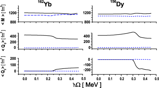
Figure 2: (Color online) The rotational behaviour of the calculated monopole and quadrupole moments. The ”double stretched” and standard values are connected by dashed and solid line, respectively.

As shown in Fig.1, the triaxiality of the mean field sets in at the rotational frequency $\Omega_{c}$ which triggers a backbending in the considered nuclei. We obtain the critical rotational frequencies, at which the first band crossing occurs, $\hbar\Omega_{c}=0.250$, $0.301$ MeV for ¹⁶²Yb, ¹⁵⁶Dy, respectively. The parameters so determined yield results in a better agreement with experiments, compared to the ones obtained in Ref.fr90 for $N\sim 90$. Moreover, our equilibrium deformations are short from being the self-consistent solutions of the HB equations. The doubly stretched quadrupole moments $\langle{\tilde{Q}}_{0}[^{\,0}_{+}]\rangle$ and $\langle{\tilde{Q}}_{2}[^{\,0}_{+}]\rangle$ are approximately zero for all values of the equilibrium deformation parameters, consistently with the stability conditions (10) (see Fig.2). Indeed, any deviation from the equilibrium values of the deformation parameters $\beta$ and $\gamma$ results into a higher HB energy. The ”double stretched” monopole moment $\langle M_{0}[^{\,0}_{+}]\rangle$ is not far from the corresponding standard one. The both values, the standard and the ”double stretched” monopole moments, are almost independent on $\Omega$. We infer from the just discussed tests that our solutions are close to the self-consistent HB ones. In contrast with our results, in Ref.fr90, the fixed parameters (deformation, pairing gap) were used for all values of the rotational frequency. In addition, the analysis of Ref.fr90, was based on the fitted moments of inertia, that were kept constant for all rotational frequencies. It is evident that such an analysis can be only used for a discussion of a general trend.

We get more insight into the backbending mechanism if consider the potential energy surface near the transition point. As is shown in Fig.3, the potential energy surface of the total mean field energy $E_{\Omega}(\beta,\gamma)=\langle H_{\Omega}\rangle$, for ¹⁵⁶Dy at $\hbar\Omega=0.300$ MeV (before the bifurcation point) exhibits the minimum for the axially symmetric shape which is lower than the minimum for strongly triaxial shape with $\gamma\approx 20^{0}$. The increase of the rotational frequency breaks the axial symmetry and a nucleus settles at the nonaxial minimum at $\hbar\Omega=0.302$ MeV (after the bifurcation point). Notice, the main difference in these minima is a strong nonaxial deformation of the one minimum in contrast to the other, while the $\beta$- deformation is almost the same.

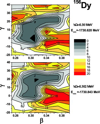
Figure 3: (Color online) The potential energy surface $E_{\Omega}(\beta,\gamma)$ for ¹⁵⁶Dy before ($\hbar\Omega=0.300$ MeV) and after ($\hbar\Omega=0.302$ MeV) the transition point. There are two local minima with almost the same $\beta$ deformation and completely different $\gamma$-deformation.

Dealing with transitional nuclei, however, the minimum becomes very shallow for a collective (around $x_{1}$ rotational axis) and non-collective (around $x_{3}$ symmetry axis) rotation as the rotational frequency increases. In fact, the energy minima for the collective ($\approx\,-1730.6$ MeV) and non-collective ($\approx\,-1730.62$ MeV) rotations are almost degenerate near the crossing point of the ground with the $\gamma$- band for ¹⁵⁶Dy (see the upper panel of the Fig. 4). The energy difference is about 15 keV near the critical rotational frequency where the backbending occurs. At the transition point, the competition between collective and non-collective rotations breaks the axial symmetry and yields nonaxial shapes. Does this behaviour correspond to a phase transition ?

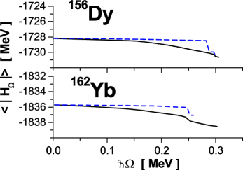
Figure 4: (Color online) The rotational dependence of the total mean field energy $E_{\Omega}(\beta,\gamma=0)=\langle H_{\Omega}\rangle$ for the axially symmetric equilibrium deformation. Results for collective ($x_{1}$ axis) and noncollective ($x_{3}$ axis) rotation are connected by solid and dashed line, respectively. Results for ¹⁵⁶Dy and ¹⁶²Yb are displayed on upper and lower panel, respectively.

First, notice that a half of an experimental value for $\gamma$-vibrations $\hbar\Omega_{K=2}/2=0.414$ MeV (at $\hbar\Omega=0$) fot is close to the collective rotational frequency $\hbar\Omega_{c}=0.301$ MeV at which the shape transition occurs. Second, let us consider an axially deformed system, defined by the Hamiltonian ${\tilde{H}}$ in the laboratory frame, that rotates about a symmetry axis z with a rotational frequency $\Omega$. The angular momentum is a good quantum number and, consequently, $[\hat{J}_{z},O_{K}^{\dagger}]=KO_{K}^{\dagger}$. Here, the phonon $O_{K}^{\dagger}$ describes the vibrational state with $K$ being the value of the angular momentum carried by the phonons $O_{K}^{\dagger}$ along the symmetry axis, $z$ axis. Thus, one obtains

$$[H_{{\Omega}},O_{K}^{\dagger}]=[{\tilde{H}}-\Omega\hat{J}_{z},O_{K}^{\dagger}]=({\tilde{\omega}}_{K}-K\Omega)O_{K}^{\dagger}\equiv\omega_{K}O_{K}^{\dagger},$$ (15)

where ${\tilde{\omega}}_{K}$ is the phonon energy of the mode K in the laboratory frame at $\Omega=0$. This equation implies that at the rotational frequency $\Omega_{cr}={\tilde{\omega}}_{K}/K$ one of the RPA frequency $\omega_{K}$ vanishes in the rotating frame (see discussion in Refs.MN93, ; HN02, ; M96, ). At this point of bifurcation we could expect the SSB effect of the rotating mean field due to the appearance of the Goldstone boson related to the multipole-multipole forces with quantum number $K$. For an axially deformed system, one obtains the breaking of the axial symmetry, since the lowest critical frequency corresponds to $\gamma$-vibrations with $K=2$ MN93 ; HN02 . The rotation around collective $x_{1}$ axis couples, however, vibrational modes with different $K$ and the critical rotational frequency is influenced by this coupling: it becomes lower. The value of $\Omega_{cr}$ can be affected by the degree of the collectivity of the vibrational excitations, as we will see below. The most important outcome from this consideration is that in the vicinity of the shape transition there is an anomalously low vibrational mode related to the deformation parameter $\gamma$.

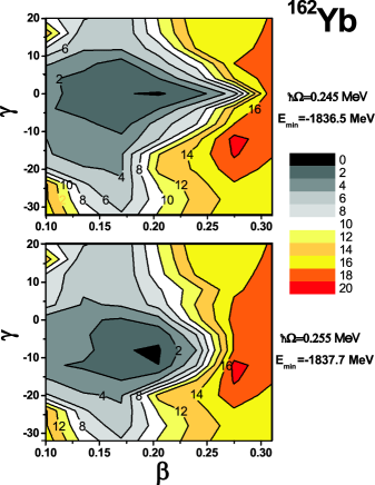
Figure 5: (Color online) The potential energy surface $E_{\Omega}(\beta,\gamma)$ for ¹⁶²Yb before ($\hbar\Omega=0.245$ MeV) and after ($\hbar\Omega=0.255$ MeV) the transition point.

For ${}^{162}Yb$ the shape transition takes place at the rotational frequency $\hbar\Omega_{c}\approx 0.25$ MeV, while the experimental bifurcation point (a half of the $\gamma$-vibrational excitation energy at $\hbar\Omega=0$) is $\hbar\Omega_{\it cr}\approx 0.45$ MeV. The energy difference at the transition point between the collective ($\approx\,-1837.7$ MeV) and the non-collective ($\approx\,-1836.6$ MeV) minima is still large $\sim 1$ MeV (see the lower panel of Fig.4). As one can see in Fig.5, the difference between the axially symmetric minimum at $\hbar\Omega=0.245$ MeV (before the transition) and the nonaxial one at $\hbar\Omega=0.255$ MeV (after the transition) for a collective rotation is about $\sim 1.2$ MeV. The deformation parameters change smoothly with the increase of the rotational frequency at the transition point (see Fig.1). It appears, that for ${}^{162}Yb$ there is a different mechanism responsible for the observed backbending.

To elucidate the different character of the shape transition from axially symmetric to the triaxial shape and its relation to a phase transition, we consider potential landscape sections in the vicinity of the shape transition. The phase transition is detected by means of the order parameter as a function of a control parameter Lan . In our case, the deformation parameters $\beta$ and $\gamma$ are natural order parameters, while the rotational frequency $\Omega$ is a control parameter that characterizes a rotational state in the rotating frame. Since we analyze a shape transition from the axially symmetric shape ($\gamma=0$) to the triaxial one ($\gamma\neq 0$), we choose only the deformation parameter $\gamma$ as the order parameter that reflects the broken axial symmetry. Such a choice is well justified, since the deformation parameter $\beta$ preserves its value before and after the shape transition in both nuclei: $\beta_{t}\approx 0.2$ for ${}^{162}Yb$ and $\beta_{t}\approx 0.31$ for ${}^{156}Dy$. Thus, we consider a mean field value of the cranking Hamiltonian, $E_{\Omega}(\gamma;\beta_{t})\equiv\langle H_{\Omega}\rangle$, for different values of $\Omega$ (our state variable) and $\gamma$ (order parameter) at fixed value of $\beta_{t}$ .

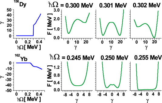
Figure 6: (Color online) The rotational dependence of the order parameter $\gamma$ and the energy surfaces sections $F(\Omega,\gamma)=E(\gamma,\beta_{t})-E_{min}$ for ${}^{156}Dy$ (top) and ${}^{162}Yb$ (bottom) before and after the transition point. The energy is given relative to the value $E_{min}=E_{\Omega}(\beta_{t},\gamma)$ at $\hbar\Omega=0.255,\,\,0.302$ MeV for ${}^{162}Yb$, ${}^{156}Dy$, respectively.

For ${}^{156}Dy$ we observe the emergence of the order parameter $\gamma$ above the critical value $\hbar\Omega_{c}=0.301$ MeV of the control parameter $\Omega$ (see a top panel in Fig.6). Below and above the transition point there is a unique phase whose properties are continuously connected to one of the coexistent phases at the transition point. The order parameter changes discontinuously as the nucleus passes through the critical point from axially symmetric shape to the triaxial one. The polynomial fit of the potential landscape section at $\hbar\Omega_{c}=0.301$ MeV yields the following expression

$$F(\Omega;\gamma)=F_{0}(\Omega)+F_{2}(\Omega)\gamma^{2}-F_{3}(\Omega)\gamma^{3}+F_{4}(\Omega)\gamma^{4},$$ (16)

where the coefficients $F_{0}(\Omega)=0.3169$ MeV, $\gamma$ in degrees and $F_{2}(\Omega)=0.12239$, $F_{3}(\Omega)=0.009199$, $F_{4}(\Omega)=1.7\times 10^{-4}$ are defined in corresponding units. We can transform this polynomial to the form

$${\bar{F}}=\frac{F(\Omega;\gamma)-F_{0}(\Omega)}{\bar{F_{0}}}\approx\alpha\frac{\eta^{2}}{2}-\frac{\eta^{3}}{3}+\frac{\eta^{4}}{4}$$ (17)

where

$${\bar{F_{0}}}=\frac{(3F_{3})^{4}}{(4F_{4})^{3}},\qquad\alpha=\frac{8F_{2}F_{4}}{9F_{3}^{2}},\qquad\eta=\frac{4F_{4}}{3F_{3}}\gamma$$ (18)

The expression (17) represents the generic form of the anharmonic model of the structural first order phase transitions in condensed matter physics (cf krum ). The condition $\partial{\bar{F}}/\partial\eta=0$ determines the following solutions for the order parameter $\eta$

$$\eta=0,\qquad\eta=\frac{1\pm\sqrt{1-4\alpha}}{2}$$ (19)

If $\alpha>1/4$, the functional ${\bar{F}}$ has a single minimum at $\eta=0$. Depending on values of $\alpha$, defined in the interval $0<\alpha<1/4$, the functional ${\bar{F}}$ manifests the transition from one stable minimum at zero order parameter via one minimum+metastable state to the other stable minimum with the nonzero order parameter. In particular, at the universal value of $\alpha=2/9$ the functional ${\bar{F}}$ has two minimum values with ${\bar{F}}=0$ at $\eta=0\rightarrow\gamma\approx 0^{0}$ and $\eta=2/3\rightarrow\gamma\approx 27^{0}$ and a maximum at $\eta=1/3\rightarrow\gamma\approx 13.5^{0}$. The correspondence between the actual value $\gamma\approx 20^{0}$ and the one obtained from the generic model is quite good. Thus the backbending in ¹⁵⁶Dy possesses typical features of the first order phase transition.

In the case of ${}^{162}Yb$ the energy $E(\Omega;\gamma)$ and the order parameter (Fig.6) are smooth functions in the vicinity of the transition point $\Omega_{c}$. This implies that two phases, $\gamma=0$ and $\gamma\neq 0$, on either side of the transition point should coincide. Therefore, for $\Omega$ near the transition point $\Omega_{c}$ we can expand our functional $F(\Omega,\gamma)=E_{\Omega}(\gamma,\beta_{t})-E_{min}$ (see Fig.6) in the form

$$F(\Omega;\gamma)=F_{1}(\Omega)\gamma+F_{2}(\Omega)\gamma^{2}+F_{3}(\Omega)\gamma^{3}+F_{4}(\Omega)\gamma^{4}+\ldots$$ (20)

The conditions of the phase equilibrium (further we restrict the expansion (20) up to the terms with $\gamma^{4}$)

$$\frac{\partial F}{\partial\gamma}=F_{1}(\Omega)+F_{2}(\Omega)2\gamma+F_{3}(\Omega)3\gamma^{2}+F_{4}(\Omega)4\gamma^{3}=0$$ (21)

$$\frac{\partial^{2}F}{\partial\gamma^{2}}=2F_{2}(\Omega)+6F_{3}(\Omega)\gamma+12F_{4}(\Omega)\gamma^{2}\geq 0\,,$$ (22)

which should be valid for all values of $\Omega$ and $\gamma$ (including $\gamma=0$), yield

$$F_{1}(\Omega)=0$$ (23)

Eqs. (21) and (22) can be rewritten as

$$2F_{2}(\Omega)\gamma+3F_{3}(\Omega)\gamma^{2}+4F_{4}(\Omega)\gamma^{3}=0$$ (24)

$$2F_{2}(\Omega)+6F_{3}(\Omega)\gamma+12F_{4}(\Omega)\gamma^{2}\geq 0$$ (25)

which implies the following inequality

$$2F_{4}(\Omega)\gamma^{2}\geq F_{2}(\Omega)$$ (26)

This inequality holds for all values of $\gamma$ (including $\gamma=0$ at $\Omega=\Omega_{c}$), which leads to $F_{2}(\Omega=\Omega_{c})\leq 0$. On the other hand, from the stability condition Eq.(22) at the transition point $\Omega_{c}$ and $\gamma=0$, we also have $F_{2}(\Omega=\Omega_{c})\geq 0$. The both inequalities can coincide only when $F_{2}(\Omega=\Omega_{c})=0$. Using the result $F_{1}(\Omega_{c})=F_{2}(\Omega_{c})=0$ and the fact that all phases at the transition point should coincide, we obtain from Eq.(21) that $F_{3}(\Omega=\Omega_{c})=0$. Assuming that $F_{3}=0$ for all $\Omega$, the minimum condition Eq.(24) yields the following solution for the order parameter

$$\gamma_{1}=0\,,\quad\gamma_{2,3}^{2}=-\frac{F_{2}(\Omega)}{2\,F_{4}(\Omega)}=\left\{\begin{array}[]{ll}\neq 0&for\,\,\Omega\neq\Omega_{c}\\ =0&for\,\,\Omega=\Omega_{c}\end{array}\right.$$ (27)

Since at the transition point $F_{2}(\Omega_{c})=0$, one can propose the following definition of the function $F_{2}(\Omega)$:

$$F_{2}(\Omega)\approx\frac{dF_{2}(\Omega)}{d\Omega}\,\left(\Omega-\Omega_{c}\right)$$ (28)

Thus, we have $\gamma\sim(\Omega-\Omega_{c})^{\nu}$ and the critical exponent $\nu=1/2$, in accord with the classical Landau theory, where the temperature is replaced by the rotational frequency.

Our extension of the Landau-type approach for rotating nuclei is nicely confirmed by the numerical results. The polynomial fit of the energy potential surfaces for ${}^{162}Yb$ (Fig.6) yields $F_{1}(\Omega)=F_{3}(\Omega)=0$ for all considered values of the rotational frequencies and $F_{2}(\Omega_{c})=0$ at $\hbar\Omega_{c}=0.25$ MeV. Moreover, in the vicinity of $\Omega_{c}$ we obtain $dF_{2}(\Omega)/\hbar d\Omega\approx-3.5$ ($F_{4}(\Omega)>0$ for all $\Omega$). In an agreement with Eqs.(27),(28), we have only the phase $\gamma=0$ for $\hbar\Omega<\hbar\Omega_{c}$ and the phase $\gamma\neq 0$ for $\hbar\Omega>\hbar\Omega_{c}$. The energy surfaces are symmetric with regard of the sign of $\gamma$ and this also supports the idea that the effective energy $F$ can be expressed as an analytic function of the order parameter $\gamma$. Thus, the backbending in ${}^{162}Yb$ can be classified as the phase transition of the second order.

II.3 Quasiparticle spectra

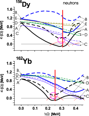
Figure 7: (Color online) Lowest quasineutron energies for ¹⁵⁶Dy (upper panel) and ¹⁶²Yb (lower panel). Thick (thin) lines are used for the positive (negative) parity states. The positive (negative) signature states are connected by solid (dashed) lines. At $\Omega=0$ the levels A, B,C, D, E correspond to the Nilsson states: 3/2[651] (the subshell $i_{13/2}$ ), 1/2[660]) (the subshell $i_{13/2}$), 3/2[521] (the subshell $h_{9/2}$), 5/2[521](the subshell $f_{7/2}$), 11/2[505] (the subshell $h_{11/2}$), respectively. The shape transition point is denoted by the vertical line. The quasicrossing is surrounded by a circle.

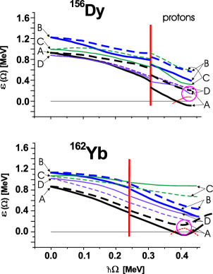
Figure 8: (Color online) Lowest quasiproton energies for ¹⁵⁶Dy (upper panel) and ¹⁶²Yb (lower panel). Thick (thin) lines are used for the negative (positive) parity states. At $\Omega=0$ the levels A,B,C,D correspond to the Nilsson states: 7/2[523] (the subshell $h_{11/2}$), 5/2[532] (the subshell $h_{11/2}$), 3/2[411](the subshell $d_{5/2}$), 5/2[413] (the subshell $g_{7/2}$), respectively, in ¹⁵⁶Dy; 7/2[523] (the subshell $h_{11/2}$), 9/2[514] (the subshell $h_{11/2}$), 5/2[402] (the subshell $d_{5/2}$), 7/2[404] (the subshell $g_{7/2}$), respectively, in ¹⁶²Yb. The shape transition point is denoted by the vertical line. The quasicrossing is surrounded by a circle.

To understand the microscopic origin of the quantum shape-phase transitions, we analyse first the quasiparticle spectra and the rotational evolution of different observables like quadrupole moments and moments of inertia. A numerical analysis of the expectation value of the nonaxial quadrupole moment

$$\langle\hat{Q}_{2}[^{\,0}_{+}]\rangle\,=\,\sum_{kl}{\langle}k|\hat{Q}_{2}[^{\,0}_{+}]|l{\rangle}\,\sum_{i}\left[{\cal V}_{i\bar{k}}{\cal V}_{i\bar{l}}\,+\,{\cal V}_{\bar{i}k}{\cal V}_{\bar{i}l}\right]$$ (29)

shows that in ¹⁶²Yb high-j neutron and proton orbitals that belong to $i_{13/2}$ and $h_{11/2}$ subshells, respectively, give the main contribution to the the expectation value. The nonaxial deformation grows due to the rotational alignment (RAL). The crossing frequencies, where the configurations with aligned quasiparticles become yrast, are order of $\Omega_{c}\approx 2\Delta/i$, where $i$ is an aligned angular momentum carried by quasiparticles. Since the neutron gap is smaller than the proton gap, one may expect that the backbending should occur due to the alignment of the quasineutron orbitals that could contribute $i\sim 8\hbar$.

We trace the rotational evolution of quasiparticle orbitals in the rotating frame (routhians) as a function of the equilibrium parameters ($\varepsilon$, $\gamma$, $\Delta$). At $\Omega=0$ each orbital is characterized by the asymptotic Nilsson quantum numbers. However, these numbers lose their validity in the rotating case due to a strong mixing. Hereafter, they are used only for convenience. The analysis of the routhians for neutrons (Fig.7) and for protons (Fig.8) indicates that the lowest quasicrossings occur: at $\hbar\Omega\approx 0.275(0.42)$ MeV for neutron (proton) system in ¹⁵⁶Dy; at $\hbar\Omega\approx 0.245(0.41)$ MeV for neutron (proton) system in ¹⁶²Yb. We recall that the shape-phase transition occurs at $\hbar\Omega_{c}\approx 0.25,0.3$ MeV in ¹⁶²Yb, ¹⁵⁶Dy, respectively. The proximity of the critical point to the two-quasiparticle neutron quasicrossing in both investigated nuclei (especially, in ¹⁶²Yb) suggests that the alignment of a pair $i_{13/2}$ is the main mechanism that drives both nuclei to triaxial shapes (cf fr90 ; scr ). This mechanism itself, however, does not provide the explanation for the different character of the shape-phase transition. We recall that the routhians exhibit the dynamics of noninteracting quasiparticles. Evidently, the interaction between quasiparticle orbitals is important and could change substantially as a function of the neutron and proton numbers. Indeed, as we will see below (see Sec.III), this explains the type of shape-phase transitions discussed in the present section.

II.4 Inertial properties

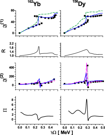
Figure 9: (Color online) The kinematical $\Im^{(1)}_{1}(\Omega)$ (top panels) and dynamical $\Im^{(2)}_{1}(\Omega)$ (second panel from the bottom) moments of inertia (in units $\hbar^{2}/MeV)$ are compared with the corresponding experimental values (filled squares). Experimental values are connected by dash-dotted line to guide eyes. The results for the kinematical moment of inertia $\Im^{(1)}_{1}(\Omega)$, with (the calculations I) and without (the calculations II) the additional term $\hat{h}_{add}$, Eq.(II.1), are connected by solid and dashed lines, respectively. The second panel (from the top) displays the ratio $R=\Im^{(1)}_{II}/\Im^{(1)}_{I}$ for each nucleus. The experimental and calculated dynamical moment of inertia $\Im^{(2)}_{1}$ (solid line) (obtained by the calculation I) are compared with the Thouless-Valatin inertia moment $\Im_{RPA}$ , Eq.(39) (dashed line). In the bottom panels the ratio, $\Pi=\Im^{(2)}_{1}/\Im^{(1)}_{1}$ is displayed.

The moment of inertia is the benchmark for microscopic models of nuclear rotation. To understand the interplay between s.p. degrees of freedom and collective effects we calculate the kinematical $\Im^{(1)}_{1}=\langle\hat{I}_{1}\rangle/\Omega$ and dynamical $\Im^{(2)}_{1}=d\langle\hat{I}_{1}\rangle/d\Omega$ moments of inertia and compare with the corresponding experimental values. The kinematical moment of inertia $\Im^{(1)}_{1}$ reflects the collective properties of the rotating mean field. The dynamical moment of inertia due to obvious relation $\Im^{(2)}_{1}=\Im^{(1)}_{1}+\Omega d\Im^{(1)}_{1}/d\Omega$ is very sensitive to structural changes of the mean field. It reflects the rearrangement of the two-body interaction upon rotation which leads to level crossings and shift in the deformation. In fact, the dynamical moment of inertia provides a definite criteria on the self-consistency of the rotating mean field when it is compared with the Thouless-Valatin moment of inertia calculated in the RPA. A full self-consistency is achieved if they are equal (see discussion in Ref. n2 ).

In Fig.9 the experimental and theoretical values of kinematical (upper panels) and dynamical (lower panels) moments of inertia are compared for ¹⁶²Yb (left panels) and ¹⁵⁶Dy (right panels). We remind that the calculations I (II) include (not include) the term $\hat{h}_{add}$, Eq.(II.1). While both calculations reproduce the rotational evolution of the kinematical moment of inertia, the agreement with the experimental data is much better for calculations I. It is interesting to note that with the increase of the rotational frequency the ratio $\Im^{(1)}_{I}/\Im^{(1)}_{II}$ increases from $\sim 50\%$ at $\hbar\Omega\sim 0.2$ MeV to $\sim 85\%$ at $\hbar\Omega\sim 0.5$ MeV. Partially, the effect of broken Galilean symmetry is reduced due to the alignment of the high-j intruder states with a large orbital momentum $l$. These states contribute to the collective angular momentum and decrease the effect of the $\vec{l}\,^{2}$ term in the Nilsson potential.

Although one observes a similar pattern for the backbending in the considered nuclei (upper panels, Fig.9), a different response of a nuclear field upon the rotation becomes more evident with the aid of the experimental dynamical moment of inertia $\Im^{(2)}=dI/d\Omega\approx 4/\Delta E_{\gamma}$ as a function of the angular frequency (see the second panel from the bottom, Fig.9). Here, $\hbar\Omega=E_{\gamma}/2$, $E_{\gamma}$ is the $\gamma$-transition energy between two neighboring states that differ on two units of the angular momentum $I$ and $\Delta E_{\gamma}$ is the difference between two consecutive $\gamma$-transitions. At the transition point $\Im^{(2)}$ wildly fluctuates with a huge amplitude in ${}^{156}Dy$, whereas these fluctuations are quite mild in ${}^{162}Yb$. This behaviour can be understood by virtue of the expansion of the microscopic moment of inertia at small rotational frequency bel

$${\Im}\approx{\cal J}_{IB}+{\cal J}_{M}+\sum_{i}\frac{\partial I}{\partial\beta_{i}}\frac{\partial{\beta_{i}}}{\partial\Omega}+...$$ (30)

The Inglis-Belyaev moment of inertia, ${\cal J}_{IB}$, neglects a residual two-body interaction between quasiparticles. Its behaviour is similar to the one of the kinematical moment of inertia, $\Im^{(1)}_{1}$. The second term ${\cal J}_{M}$ is a Migdal moment of inertia mig , resulting from the effect of rotation on the residual two-body interaction and, in particular, on the pairing interaction. In our calculations the pairing gaps change smoothly in accord with the phenomenological prescription, Eq.(9). The third term describes the variation of the self-consistent mean field, namely, the change of the deformation $(\beta_{1,2}\equiv\beta,\gamma$) under rotation. Therefore, a drastic change of the mean field configuration (namely, $\gamma$ -deformation) in ¹⁵⁶Dy (see Fig.6, top panels) explains large fluctuations of the dynamical moment of inertia at the transition point. In contrast, the smooth behaviour of the function $F$ at the transition point (see Fig.6, bottom panels) implies a small amplitude of fluctuations of the dynamical moment of inertia in ¹⁶²Yb. The magnitude of fluctuations can be traced by means of the ratio $\Pi={\Im}^{(2)}_{1}/{\Im}^{(1)}_{1}$ as a function of the rotational frequency (see the bottom panel in Fig.9). While this ratio is about $\Pi\sim 2$ at the transition point in ¹⁶²Yb, in ¹⁵⁶Dy it is much larger $\Pi\sim 8$. Referring to above analysis of the mean field solutions, we can formulate the empirical rule to detect the order of the quantum shape-phase transition at the backbending: if the ratio $\Pi={\Im}^{(2)}/{\Im}^{(1)}>>1$ at the transition point, the shape transition can be associated with a first order phase transition.

The nature of the backbending becomes more evident by dint of the RPA analysis presented below. For a completeness, we also compare the Thouless-Valatin moment of inertia (the definition is presented in Sec.III) with the dynamical moment of inertia $\Im^{(2)}_{1}$ calculated in the mean field approximation. Notice, that all three terms in Eq.(30) are included into the Thouless-Valatin moment of inertia, ${\Im}_{RPA}={\Im}$, calculated in the RPA (see, for example, the discussion in Ref.n2, for the exact model without pairing), which is valid at large rotational frequencies as well. One can observe a remarkable agreement between experimental, mean field and CRPA results. The agreement between the mean field and CRPA results confirms a good accuracy of our mean field calculations. This agreement, on the other hand, demonstrates a validity of our CRPA approach in the backbending region, at least, for the description of the spectrum.

III Quadrupole Collective excitations

III.1 Quasiparticle RPA in rotating systems

In this section we discuss the RPA results to get a further insight into the backbending mechanism. By means of a generalized Bogoliubov transformation, we express the Hamiltonian given by Eq. (1) in terms of quasiparticle creation ($\alpha^{\dagger}_{i}$) and annihilation ($\alpha_{i}$) operators. We then face with the RPA equations of motion, written in the form KN ; JK

$$[H_{\Omega},P_{\nu}]\, = \,i\,\hbar\omega_{\nu}^{2}\,X_{\nu},\qquad[H_{\Omega},X_{\nu}]\,=\,-i\,\hbar\,P_{\nu},$$ (31)

$$[X_{\nu},P_{\nu^{\prime}}]\,=\,i\hbar\delta_{\nu\,\nu^{\prime}},$$

where $X_{\nu}$, $P_{\nu}$ are, respectively, the collective coordinates and their conjugate momenta. The solution of the above equations yields the RPA eigenvalues $\hbar\omega_{\nu}$ and eigenfunctions

$$|\nu>\,=\,O_{\nu}^{\dagger}|RPA> = \frac{1}{\sqrt{2}}\,\Bigl{(}\,\sqrt{\frac{\omega_{\nu}}{\hbar}}\,X_{\nu}\,-\,\frac{i}{\sqrt{\hbar\omega_{\nu}}}\,\hat{P}_{\nu}\,\Bigr{)}|RPA>$$ (32)

$$= \sum_{\mu}\Bigl{(}\psi_{\mu}^{\nu}b^{\dagger}_{\mu}-\phi^{\nu}_{\mu}b_{\mu}\Bigr{)}|RPA>,$$

where $\mu=({k{\bar{l}}})$ or $({kl},{\bar{k}}{\bar{l}})$. Here, the boson-like operators $b^{+}_{k\bar{l}}=\alpha^{+}_{k}\alpha^{+}_{\bar{l}},b^{+}_{kl}=\alpha^{+}_{k}\alpha^{+}_{l},b^{+}_{\bar{k}\bar{l}}=\alpha^{+}_{\bar{k}}\alpha^{+}_{\bar{l}}$ are used. The first equality introduces the positive signature boson, while the other two determine the negative signature ones. These two-quasiparticle operators are treated in the quasi-boson approximation (QBA) as an elementary bosons, i.e., all commutators between them are approximated by their expectation values with the uncorrelated HB vacuum RS . The corresponding commutation relations can be found in Ref.KN, . In this approximation any single-particle operator $\hat{F}$ can be expressed as $\hat{F}=\langle F\rangle+\hat{F}^{(1)}+\hat{F}^{(2)}$ where the second and third terms are linear and bilinear order terms in the boson expansion. We recall that in the QBA one includes all second order terms into the boson Hamiltonian such that $(\hat{F}-\langle F\rangle)^{2}=\hat{F}^{(1)}\hat{F}^{(1)}$. The positive and negative signature boson spaces are not mixed, since the corresponding operators commute and $H_{\Omega}=H_{\Omega}(r=+1)+H_{\Omega}(r=-1)$. Consequently, we can solve the eigenvalue equations (31) for $H_{\Omega}(+)$ and $H_{\Omega}(-)$, separately.

The symmetry properties of the cranking Hamiltonian yield

$$[\,H_{\Omega}(+)\,,\,N_{\tau=n,p}\,]_{RPA}\,=\,0,\,\,\,\,[H_{\Omega}(+)\,,\,I_{1}\,]_{RPA}=0.$$ (33)

The presence of the cranking term in Hamiltonian (1) leads to the following equation

$$[H_{\Omega}(-),\Gamma^{\dagger}]=\hbar\Omega\Gamma^{\dagger},$$ (34)

where $\Gamma^{\dagger}=(I_{2}+iI_{3})/\sqrt{2\langle I_{1}\rangle}$ and $\Gamma=(\Gamma^{\dagger})^{\dagger}=(I_{2}-iI_{3})/\sqrt{2\langle I_{1}\rangle}$ fulfill the commutation relation

$$[\Gamma,\Gamma^{\dagger}]=\hbar.$$ (35)

According to Eqs.(33), we have two Nambu-Goldstone modes, one is associated with the violation of the conservation law for a particle number, the other is a positive signature zero frequency rotational solution associated with the breaking of spherical symmetry. Eq.(34), on the other hand, yields a negative signature redundant solution of energy $\omega_{\nu}=\Omega$, which describes a collective rotational mode arising from the symmetries broken by the external rotational field (the cranking term). Eqs. (33) and (34) ensure the separation of the spurious or redundant solutions from the intrinsic ones. They would be automatically satisfied if the single-particle basis was generated by means of a self-consistent HB calculation. As we shall show, they are fulfilled with a good accuracy also in our, not fully self-consistent, HB treatment.

We recall that the yrast states possess the positive signature quantum number. Obviously, SSB effects of the mean field are related to Nambu-Goldstone modes of the same signature. Therefore, in this paper our analysis is focused upon positive signature RPA excitations.

The positive signature Hamiltonian consists of the following terms

$$\hat{H}_{\Omega}[r=+1]=\sum_{ij}E_{i\bar{j}}b^{+}_{i\bar{j}}b_{i\bar{j}}-\sum_{\tau=N,P}G_{\tau}\hat{P}_{\tau}^{(1)^{+}}\hat{P}_{\tau}^{(1)}$$ (36)

$$- 1/2\sum_{T=0,1}\,\kappa_{0}[T](\tilde{M}^{(1)}[^{T}_{r=+1}])^{2}-\frac{1}{2}\kappa_{\sigma}\sum_{T=0,1}(\tilde{s}_{1}^{(1)}[^{T}_{r=+1}])^{2}$$

$$- \frac{1}{2}\sum_{T=0,1}\,\kappa_{2}[T]\sum_{\mu=0,1,2}(\tilde{Q}^{(1)}_{\mu}[^{T}_{r=+1}])^{2}$$

Here, $E_{i\bar{j}}=\varepsilon_{i}+\varepsilon_{\bar{j}}$ are two-quasiparticle energies and the definition of matrix elements of the operators involved in the Hamiltonian (36) can be found in Ref.JK, . The solution of the equations of motion, Eq.(31), leads to the following determinant of the secular equations

$${\cal F}(\omega_{\nu})=\det~{}({\bf R}-\frac{\bf 1}{2c}~{}),$$ (37)

with a dimension $n=12$ and $c=\kappa_{0},\kappa_{2}$ or $G_{\tau}$. The matrix elements $R_{km}(\omega_{\nu})=\sum_{\mu}q_{k,\mu}q_{m,\mu}C_{\mu}^{km}/(E_{\mu}^{2}-\omega_{\nu}^{2})$ involve the coefficients $C_{\mu}^{km}=E_{\mu}$ or $\omega_{\nu}$ for different combinations of matrix elements $q_{k,\mu}$ (see details in Refs.KN, ; JK, ). The zeros of the function ${\cal F}(\omega_{\nu})=0$ yield the CRPA eigenfrequencies $\omega_{\nu}$. Once the RPA solutions are found, the Hamiltonian (36) can be written in terms of the collective modes ($\hat{\mathit{X}_{\nu}}$, $\hat{\mathit{P}_{\nu}}$)

$$\hat{H}_{\Omega}[r] = \frac{1}{2}\sum_{\nu}\left(\hat{\mathit{P}}^{2}_{\nu}+\omega^{2}_{\nu}\hat{\mathit{X}}^{2}_{\nu}\right)=\sum_{\nu(\omega_{\nu}\neq 0)}\hbar\omega_{\nu}\left(Q^{+}_{\nu}Q_{\nu}+\frac{1}{2}\right)$$ (38)

$$+ \frac{1}{2}g_{I_{1}}\hat{\mathit{I}}^{(1)^{2}}_{1}+\frac{1}{2}\sum_{\tau}g_{N_{\tau}}\hat{\mathit{N}}^{(1)^{2}}_{\tau}$$

where $g_{I_{1}}=1/\Im_{RPA}$, $g_{N_{\tau}}$ are the Thouless-Valatin moment of inertia and the nucleus mass, respectively, determined in the uniform rotating (UR) frame. The general derivation of the mass parameters $g_{I_{1}}$ and $g_{N_{\tau}}$ can be found in Refs.KN, ; 29, . In particular, for the moment of inertia we have

$$\Im_{RPA}=\frac{detA}{detB}$$ (39)

where $A_{kl}$ is the matrix (the dimension $n=10$) given by the part of the matrix ${\cal F}_{kl}(\omega=0)$ corresponding to the s.p. operators $k$, and $l$ involved in $\hat{H}[r=+1]$ with the structure $(b^{+}_{i\bar{j}}+b_{i\bar{j}})$ type. The matrix $B_{kl}$ (with the dimension $n=11$) is given by matrix $A_{kl}$ with additional one column and row involving $0$ and sums $\pm\sum_{\mu=i\bar{j}}\frac{f^{(k)}_{\mu}J^{(1)}_{\mu}}{E_{\mu}}$, $(k=1,...,8)$ where $J^{(1)}_{i\bar{j}}$ are quasiparticle matrix elements of the operator $\hat{I}_{1}$ (see Ref.29, for details).

Transition probabilities for $X\lambda$ transition $|I\nu>\rightarrow|I^{\prime}\nu^{\prime}>$ between two high-spin states is given by expression

$$B(X\lambda;I\nu\rightarrow I^{\prime}\nu^{\prime})=$$ (40)

$$(I\,I\,\lambda\,\mu_{1}\,|\,I^{\prime}\,I^{\prime})^{2}|<\nu^{\prime}|\hat{\cal M}^{(1)}(X\lambda;\mu_{1}=I^{\prime}-I)|\nu>|^{2}$$

At high spin limit ($I>>\lambda$, $I^{\prime}>>\lambda$), this expression takes the form mar1

$$B(X\lambda;I\nu\rightarrow I^{\prime}yr)\simeq$$ (41)

$$|<RPA|\left[Q_{\nu},\hat{\cal M}^{(1)}(X\lambda;\mu_{1}=I^{\prime}-I)\right]|RPA>|^{2}$$

for the transition from one phonon states into the yrast line states. Here, $\hat{\cal M}^{(1)}(X\lambda\mu_{1})$ is the linear boson part of the corresponding transition operator of type $X$, multipolarity $\lambda$ and the projection $\mu_{1}$ onto the rotation axis (the first axis of the UR system). The commutator in (41) can be easily expressed in terms of phonon amplitudes $\psi^{(\nu)}_{\mu}$, $\phi^{(\nu)}_{\mu}$ ($\mu=i\bar{j}$ or $ij,\bar{i}\bar{j})$ and $\mid RPA\rangle$ denotes the RPA vacuum (yrast state) at the rotational frequency $\Omega$. The multipole operator in the rotating frame is obtained from the corresponding one in the laboratory frame according to the prescription mar1

$${\cal M}(X\lambda\mu_{1})=\sum_{\mu_{3}}\,\,{\cal D}^{\lambda}_{\mu_{1}\mu_{3}}(0,\frac{\pi}{2},0)\,\,{\cal M}(X\lambda\mu_{3}).$$ (42)

Taking into account that $<\nu|\hat{M}^{(E)}_{2\mu_{3}=0,2}[+]|\nu>=\langle|\hat{M}^{(E)}_{2\mu_{3}=0,2}[+]|\rangle$ holds in the first RPA order and Eq.(42), we have

$$B(E2;I\nu\rightarrow I-2\,\nu)=\left|<\nu|\hat{\cal M}^{(1)}(E2;\mu_{1}=2)|\nu>\right|^{2}$$ (43)

$$= \frac{1}{2}\left|\frac{\sqrt{3}}{2}\langle|\hat{M}^{(E)}_{2\mu_{3}=0}[+]|\rangle-\frac{1}{2}\langle|\hat{M}^{(E)}_{2\mu_{3}=2}[+]|\rangle\right|^{2}$$

Using the $\beta$ - $\gamma$ deformation parameterization, Eq.(13), and the oscillator value for the isoscalar quadrupole constant, $\kappa_{2}[0]\approx\frac{4\pi}{5}\frac{m\omega^{2}_{0}}{<r^{2}>}\approx\frac{4\pi}{3A}m\omega^{2}_{0}R^{2}$ ($R=1.2A^{1/3}fm$), we obtain an approximate expression

$$B(E2;I\,yr\,\rightarrow\, I-2\,yr)\approx$$ (44)

$$\frac{1}{2}\frac{9e^{2}Z^{2}}{16\pi^{2}}R^{4}\beta^{2}\cos^{2}(\frac{\pi}{6}-\gamma)$$

Here, we use $\hat{M}^{(E)}=(eZ/A)\hat{M}$. From this expression one can conclude that the change of the $\gamma$-deformation from zero to $\pi/6$ will increase the transition probability. The negative sign of $\gamma$-deformation results in the decrease of this probability. As we will see below, this expression is useful for the analysis of the experimental data.

III.2 Determination of the residual interaction strengths

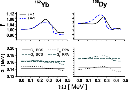
Figure 10: (Color online) The ratio $f=\kappa_{\it cal}/\kappa_{\it osc}$ between actual and oscillator isoscalar quadrupole strength constants for the positive and negative signature is displayed on the upper panel. On the lower panel, the actual and the BCS pairing constants $G_{N}$ and $G_{P}$ (see the definition in the text) are shown. All actual values used in the calculations are obtained as to fulfill the RPA equations, Eqs.(33)-(34), for the spurious or redundant modes. The results correspond to the calculation I, when the term $\hat{h}_{add}$ (II.1), that restores the local Galilean invariance broken in the Nilsson potential, is included.

In order to determine the strength $\kappa$ of the monopole and quadrupole interactions, we start with the oscillator values ds

$$\kappa_{\lambda}[0]=\frac{4\pi}{2\lambda+1}\frac{m\omega_{0}^{2}}{A<{\tilde{r}}^{2\lambda-2}>},\,\,\,\,\,\,\,\kappa_{\lambda}[1]=-\frac{\pi V_{1}}{A<{\tilde{r}}^{2\lambda}>}\,.$$ (45)

For instance, the isoscalar strength follows from enforcing the Hartree self-consistent conditions. We then change slightly these strengths and the pairing interaction constants $G_{\tau}$ at each rotational frequency, while keeping constant the $\kappa[1]/\kappa[0]$ ratio ($\kappa_{0}[1]/\kappa_{0}[0]\approx-18$, $\kappa_{2}[1]/\kappa_{2}[0]\approx-3.6$), so as to fulfill the RPA equations (33)-(34) for the spurious or redundant modes.

The rotational dependence of these parameters is relatively weak. The ratio between actual and oscillator value for the isoscalar quadrupole constant is displayed in Fig.10. For comparison, the BCS values $G_{\tau}$, $G_{N}\approx 22.5/A$ MeV, $G_{P}\approx 26.5/A$ MeV, obtained from the systematic of pairing gaps (see Ref.33, ), are shown in Fig.10 as well. Surprisingly, the difference between actual values and the latter ones is mild. However, the determination of $\kappa_{2}[0]$ and $G_{\tau}$ is a tedious task, since a tiny change of the strength parameters leads to large shifts in energies of spurious modes. The constants so determined differ from the HO ones by 5-10% at most. For the spin-spin interaction, we use the generally accepted strengths 34

$$\kappa_{\sigma}[0]\,=\,\kappa_{\sigma}[1]\,=\,-28\,\frac{4\pi}{A}\,MeV$$

for all rotational frequencies. The spin-spin interaction does not influence the position of Nambu-Goldstone modes and, therefore, does not play any role in the self-consistent determination of the quadrupole strength constants. Finally, we adopted bare charges to compute the $E2$ strengths and a quenching factor $g_{s}=0.7$ for the spin gyromagnetic ratios to compute the $M1$ strengths.

By using the above set of parameters, it was possible not only to separate the spurious and rotational solutions from the intrinsic modes, but also to reproduce the experimental dependence of the lowest $\beta$- and $\gamma$-bands on the rotational frequency $\hbar\Omega$ and, in particular, to observe the crossing of the $\gamma$- band with the ground band in correspondence with the onset of triaxiality.

Concluding the discussion about our calculation scheme, we should mention some drawbacks of our approach. One of the disadvantage is the CRPA breaks down at the transition point when $\Delta_{p}$ or $\Delta_{n}$ vanish mar1 . We have avoided this problem by means of the phenomenological prescription for the rotational dependence of the pairing gap (see Section II). In principle, projection methods should be used in the transition region in order to calculate transition matrix elements. In the case of the phase transition of the first order we run into the problem of the formidable overlap integral. A theory of large amplitude motion would provide a superior means to solve this problem.

However, in contrast to the standard RPA calculations, where the residual strength constants are fixed for all values of $\Omega$ (see e.g. mat1 ; mat2 ), we determine the strength constants for each value of $\Omega$ by the requirement of the validity of the conservation laws. This enables us to overcome the instability of the RPA calculations at the transition region, at least, for the excitations (see also discussion for quantum dots in Ref.llor1, ). Although the amplitudes $\phi^{(\nu)}_{\mu}$ (see Eq.(32)) are higher for the RPA modes in the transition region than in other regions, the relation $|\phi^{(\nu)}_{\mu}|<|\psi^{(\nu)}_{\mu}|$ is still valid to hold the QBA. And least but not last, the CRPA becomes quite effective at high spins, when the pairing correlations are suppressed.

III.3 Positive signature excitations in the rotating frame

In this section we analyse the spectral and decay properties of the positive signature states. Transition probabilities represent the most challenging task, since they are sensitive about the wave function structure of the considered state and, therefore, exhibit hidden drawbacks of a theory.

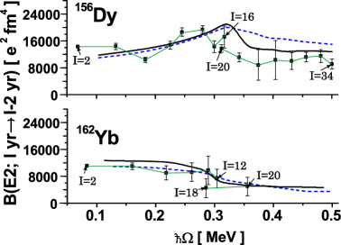
Figure 11: (Color online) Reduced transition probabilities $B(E2;I\,yr\,\rightarrow\,I-2\,yr)$ along the yrast line. Experimental data (filled squares) are connected with a thin line to guide eyes. The results of calculations by means of Eq.(43) and of Eq.(44) are connected by solid and dashed lines, respectively.

Experimental values of $B(E2,\,I\,\nu\,\rightarrow\,I^{\prime}\,yr)$ are deduced from the half life of the yrast states nndc using the standard, long wave limit expressions $B(E2,i\,\rightarrow\,f)=\ P(i\,\rightarrow\,f)/(1.223\times 10^{9}E^{5}_{\gamma})\,\,(e^{2}$ fm${}^{4})$ BM1 ; RS . Here, the transition energy $E_{\gamma}$ is in MeV and the absolute transition probability $P(i\,\rightarrow\,f)=\ln 2/T(i\,\rightarrow\,f)$ is the related to the half life $T(i\,\rightarrow\,f)$ (in seconds). For ¹⁵⁶Dy the yrast energies and corresponding half lifes are known up to the momentum $I\approx 40\hbar$. For ¹⁶²Yb yrast energies are observed up to $I\approx 28\hbar$ but half lifes were measured only up to $I\approx 20\hbar$. While the cranking approach should be complemented with a projection technique in the backbending region due large fluctuation of the angular momentum (cf Ref.RS, ), its validity becomes much better at high spins. The agreement between calculated and experimental values of intraband $B(E2)$ transitions along the yrast line is especially good after the transition point.

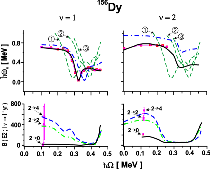
Figure 12: (Color online) ¹⁵⁶Dy. Experimental (filed square) and calculated excitation energies in the rotating frame $\hbar\omega_{\nu}=R_{\nu}(\Omega)-R_{yr}(\Omega)$ (upper panel) and reduced transition probabilities $B(E2;I\,\nu\,\rightarrow\,I^{\prime}\,yr)$ (lower panel) for two lowest RPA solutions, $\nu=1$ (left) and $\nu=2$ (right), as a function of the angular frequency $\hbar\Omega$. The results for excitations, calculated with and without the term $\hat{h}_{add}$, Eq. (II.1), are connected by solid and dash-dotted lines, respectively. The experimental values for the transitions are indicated by arrows. The tansitions with $\Delta I=2,0,-2$ are connected by solid, dash-dotted and dashed lines, respectively. Two-quasiparticle energies, indicated by arrows with numbers 1, 2, and 3 in circles, originate from two s.p. Nilsson states ($n\bar{n}\,\frac{3}{2}[651]\,\,\frac{3}{2}[651]$), ($p\bar{p}\,\frac{7}{2}[523]\,\,\frac{7}{2}[523]$), and ($n\bar{n}\,\frac{1}{2}[530]\,\,\frac{5}{2}[523]$) at $\Omega=0$ and $\Delta_{\tau}=0$.

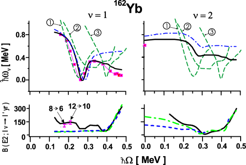
Figure 13: (Color online) ¹⁶²Yb. The same as for Fig.12. Two-quasiparticle energies, indicated by arrows with numbers 1, 2, and 3 in circles, originate from two s.p. Nilsson states ($n\bar{n}\,\frac{3}{2}[651]\,\,\frac{3}{2}[651]$), ($n\bar{n}\,\frac{3}{2}[521]\,\,\frac{3}{2}[521]$), and ($p\bar{p}\,\frac{7}{2}[523]\,\,\frac{7}{2}[523]$) at $\Omega=0$ and $\Delta_{\tau}=0$.

Experimental data are compared with the results of calculations (a) by means of Eq.(43) and calculations (b) by means of Eq.(44) (see Fig.11). In the calculations (a) we use the mean field values for the quadrupole operators. In the calculations (b) these values have been replaced by the deformation parameters via Eq.(13) and we use the oscillator value for the quadrupole strength constant. The calculations (a) evidently manifest the backbending effect obtained for the moments of inertia (see Fig.9) at $\hbar\Omega_{c}\approx 0.25,\,0.3$ MeV for ¹⁶²Yb and ¹⁵⁶Dy, respectively. Thus, the use of the self-consistent expectation values $\langle|\hat{M}^{(E)}_{2\mu_{3}}[+]|\rangle$ is crucial to reproduce the experimental behaviour of the yrast band decay. The calculations (b) (Eq.(44)) reproduce the experimental data with less accuracy. However, these results also catch on the correlation between the sign of the $\gamma$-deformation and the behaviour of the transition probability. The onset of the positive (negative) values of $\gamma$-deformation lead to the increase (decrease) of the transition probability along the yrast line. This fact nicely correlates with the experimental data.

To analyse experimental data on low lying excited states near the yrast line we construct the Routhian function for each rotational band $\nu$ ($\nu=yrast,\beta,\gamma,...$)

$$R_{\nu}=E_{\nu}(\Omega)-\hbar\Omega I(\Omega),\quad\quad\Omega(I)=\frac{E_{\nu}(I+2)-E_{\nu}(I)}{2}$$ (46)

and define the experimental excitation energy in the rotating frame $\hbar\omega_{\nu}^{\it exp}=R_{\nu}(\Omega)-R_{yr}(\Omega)$ n87 . This energy can be directly compared with the corresponding solutions $\hbar\omega_{\nu}$ of the RPA secular equations for a given rotational frequency $\Omega$. We remind that our vacuum states are adiabatic quasiparticle configurations that correspond to the occupied orbitals at a given rotational frequency.

The first lowest positive signature RPA solutions ($\nu=1$) create an excited band built on the yrast line. In both nuclei, this band is close to the experimental $\gamma$-excitations with even spin at small rotational frequency $\Omega$ (see Figs.12, 13). In the low-spin region, the transitions $B(E2;\,I\nu=1\,\rightarrow\,I^{\prime}yr)$ are large and RPA solutions exhibit a strong collective nature of the $\gamma$ - band (Weisskopf units are $B(E2)_{W}\,=\,49.9,\,52.5\,e^{2}fm^{4}$ for ${}^{156}Dy$, ${}^{162}Yb$, respectively) in both nuclei. The collective character of the low-spin part of the $\gamma$ - bands is manifested in the phonon structure that is composed by a few two-quasiparticle components (see below and Tables I,II).

In ¹⁵⁶Dy the RPA results, obtained with the term $\hat{h}_{add}$ (II.1), reproduce quite well the rotational behaviour of the lowest excitations associated with the collective $\gamma$-vibrations. We also obtain a good agreement with the experimental value of the critical rotational frequency $\hbar\Omega_{cr}\approx 0.324$ MeV, at which this mode disappear in the rotating frame. This results is very close to the critical rotational frequency $\hbar\Omega_{c}\approx 0.3$ MeV (see Fig.6), where the backbending occurs (see Eq.(15) and discussion in Sec. II). In accordance with the phenomenological theory of the first order phase transitions discussed in Section II, this soft mode creates a shape transition from the axial to the nonaxial shapes. We emphasize that without the term $\hat{h}_{add}$ the transition point is located considerably higher than the experimental one. In ¹⁶²Yb, the results with and without this term are very close (see Fig.13). In contrast to ¹⁵⁶Dy, in ¹⁶²Yb the crossing, is determined by a single two-quasiparticle state (see Table I at $I=10\hbar$). The term $\hat{h}_{add}$ results in a collective effect to the mean field solution, while its contribution to a single, two-quasiparticle energy $E_{\mu}$ is weak. As discussed in Sec. II, the effect of this term is also reduced due to the alignment.

Table 1: The structure of the $\nu=1$ positive signature phonon in ${}^{162}Yb$.

$I=2\,$	$n\bar{n}\,\frac{3}{2}[651]\,\,\frac{1}{2}[660]\,49$%	$n\bar{n}\,\frac{3}{2}[651]\,\,\frac{3}{2}[651]\,\,40$%	$p\bar{p}\,\frac{7}{2}[523]\,\,\frac{11}{2}[505]\,\,13$%
$I=6\,$	$n\bar{n}\,\frac{3}{2}[651]\,\,\frac{3}{2}[651]\,\,72$%	$n\bar{n}\,\frac{3}{2}[651]\,\,\frac{1}{2}[660]\,\,20$%	$p\bar{p}\,\frac{7}{2}[523]\,\,\frac{7}{2}[523]\,\,\,4$%
$I=10$	$n\bar{n}\,\frac{3}{2}[651]\,\,\frac{3}{2}[651]\,\,96$%	$p\bar{p}\,\frac{7}{2}[523]\,\,\frac{7}{2}[523]\,\,\,2$%	$n\bar{n}\,\frac{1}{2}[651]\,\,\frac{1}{2}[660]\,\,\,1$%
$I=14$	$n\bar{n}\,\frac{3}{2}[651]\,\,\frac{3}{2}[651]\,\,85$%	$n\bar{n}\,\frac{3}{2}[521]\,\,\frac{3}{2}[521]\,\,\,7$%	$p\bar{p}\,\frac{7}{2}[523]\,\,\frac{7}{2}[523]\,\,\,7$%
$I=18$	$n\bar{n}\,\frac{3}{2}[521]\,\,\frac{3}{2}[521]\,\,70$%	$p\bar{p}\,\frac{3}{2}[651]\,\,\frac{3}{2}[651]\,\,21$%	$p\bar{p}\,\frac{7}{2}[523]\,\,\frac{7}{2}[523]\,\,\,5$%

Table 2: The structure of the $\nu=1$ positive signature phonon in ${}^{156}Dy$.

$I=2\,$	$n\bar{n}\,\frac{3}{2}[651]\,\,\frac{1}{2}[660]\,\,48$%	$p\bar{p}\,\frac{7}{2}[523]\,\,\frac{7}{2}[523]\,\,17$%	$n\bar{n}\,\frac{1}{2}[530]\,\,\frac{5}{2}[523]\,\,16$%
$I=6\,$	$n\bar{n}\,\frac{3}{2}[651]\,\,\frac{3}{2}[651]\,\,63$%	$p\bar{p}\,\frac{1}{2}[550]\,\,\frac{1}{2}[541]\,\,15$%	$n\bar{n}\,\frac{1}{2}[530]\,\,\frac{5}{2}[523]\,\,13$%
$I=10$	$n\bar{n}\,\frac{3}{2}[651]\,\,\frac{3}{2}[651]\,\,60$%	$p\bar{p}\,\frac{1}{2}[550]\,\,\frac{7}{2}[523]\,\,17$%	$n\bar{n}\,\frac{1}{2}[530]\,\,\frac{5}{2}[523]\,\,14$%
$I=14$	$n\bar{n}\,\frac{3}{2}[651]\,\,\frac{3}{2}[651]\,\,65$%	$p\bar{p}\,\frac{7}{2}[523]\,\,\frac{7}{2}[523]\,\,18$%	$n\bar{n}\,\frac{3}{2}[530]\,\,\frac{5}{2}[523]\,\,13$%
$I=18$	$n\bar{n}\,\frac{3}{2}[651]\,\,\frac{3}{2}[651]\,\,71$%	$p\bar{p}\,\frac{7}{2}[523]\,\,\frac{1}{2}[541]\,\,12$%	$n\bar{n}\,\frac{1}{2}[530]\,\,\frac{5}{2}[523]\,\,13$%

In Tables 1, 2 we present the contribution $n_{i\bar{j}}(\nu=1)=(\psi^{(\nu=1)}_{i\bar{j}})^{2}-(\varphi^{(\nu=1)}_{i\bar{j}})^{2}$ of main two-quasiparticle components to the norm $\sum_{ij}n_{i\bar{j}}(\nu=1)\,=\,1$ of the RPA solution $\hbar\omega_{\nu=1}$ as a function of the angular momentum (rotational frequency). The collectivity is weaker in ¹⁶²Yb than in ¹⁵⁶Dy. With the increase of the rotational frequency, in ¹⁶²Yb the phonon loses the collective nature and a single, two-quasiparticle neutron component ($i\bar{j}\,=\,n\bar{n}\,\frac{3}{2}[651]\,\frac{3}{2}[651]$) is dominant in the transition region. At the crossing point its weight reaches 96% and $B(E2;\,I\nu=1\rightarrow I^{\prime}yr)$ values falls down to their s.p. values $B(E2)_{W}$. The transition from axially symmetric to nonaxial shapes occurs due to the alignment of this two-quasiparticle component along the axis of the collective rotation. There the SSB effects display a single-particle mechanism.

In contrast with ¹⁶²Yb, in ${}^{156}Dy$ the phonon excitation $\hbar\omega_{\nu=1}$ remains collective even in the backbending region (see Table 2 for $I\approx 14\hbar$). The $B(E2;\,I\nu=1\rightarrow I^{\prime}yr)$ values decrease with the increase of the rotational frequency but the phonon holds the collectivity even at the transition point $\hbar\Omega_{c}=0.301$ MeV. Although two-quasiparticle states align their angular momenta along the axis x (collective rotation), the axial symmetry persists till the transition point (see also discussion in Ref.JK1, ). The mode blocks a transition to the triaxial shape. At the transition point the phonon becomes anomalously soft and we obtain a change of the symmetry of the HB solution from axially symmetric to nonaxial shape. Thus, the SSB effect occurs due to vanishing of the collective $\gamma$-vibrational excitations in the rotating frame.

The second positive signature nonspurious RPA solution, $\hbar\omega_{\nu=2}$ can be associated with the $\beta$ - band at small rotational frequencies. For ¹⁵⁶Dy the agreement between the experimental $\hbar\omega_{\beta}$ and the calculated $\hbar\omega_{\nu=2}$ is good (see Fig.12). In ¹⁶²Yb only one lowest level of $\beta$-band is experimentally observed at $\hbar\Omega=0$ MeV and it is very close to the calculated value of the $\hbar\omega_{\nu=2}$. Our results may be considered as a theoretical prediction for the behaviour of the $\beta$-band at larger rotational frequencies.

IV Summary

We develop a practical method based on the cranked Nilsson potential with separable residual interactions for the analysis of the low-lying excitations near the yrast line. In contrast to previous studies of low-lying excitations at high spins (cf Refs.mat1 ; mat2 ), we pay a special attention to the self-consistency between mean field results and description of low-lying excitations in the RPA. We accounted for the $\Delta N=2$ coupling in generating the Nilsson states and included the Galilean invariance restoring piece according to the prescription of Ref.nak, . Moreover, we enforced the HB stability conditions, provided by Eq.(10), that yield deformation parameters very close to the self-consistent values. Finally, we fixed the strength parameters of the interaction so as to ensure the separation of the spurious modes from the intrinsic excitations at each rotational frequency. This way we provide a reliable approach to study the spontaneous breaking effects of continuous symmetries of the rotating mean field. Note that even in self-consistent calculations with effective forces (Gogny or Skyrme type) this separation is not guaranteed due to a finite size of the configuration space. One needs an extended configuration space to ensure a good separation of a spurious contribution to the intrinsic wave function (see, for example, discussion in Ref.llor1, ).

We analyse the rotational properties of the yrast and low-lying positive signature excitations in the transitional nuclei ¹⁵⁶Dy and ¹⁶²Yb undergoing the backbending. The agreement between our results and experimental data is remarkable. We obtain a simple expression, Eq.(44), for the reduced transition probability along the yrast line, that naturally explains the increase/decrease of $B(E2)$-transitions due to the shape transition from axially symmetric to nonaxial shapes with different sign of the $\gamma$-deformation of the rotating mean field. The magnitude of the B(E2) transition probability along the yrast line increases with the angular momentum and drops down at the transition point in both nuclei. We demonstrate a good agreement between the dynamical moment of inertia calculated at the mean field level and the Thouless-Valatin moment of inertia calculated in the RPA in the realistic calculations. This is one of the stringent test of the self-consistency between mean field and RPA calculations. Our RPA analysis reveals a mechanism of the backbending phenomena in rotating nuclei, which is caused by the disappearance of the $\gamma$-vibrations in the rotating frame and following alignment of the two-quasiparticle components of the $\gamma$-phonon.

We found that in axially symmetric nuclei in the ground state two types of quantum phase transitions may occur with rotation, which are associated with the backbending. In ¹⁵⁶Dy we obtain that $\gamma$-vibrational excitations ($K=2$) tend to zero in the rotating frame with the increase of the rotational frequency $\Omega$, in close agreement with experimental data. Although two-quasiparticle states align their angular momenta along the axis x (collective rotation), the axial symmetry persists, since the vibrational mode blocks a transition to the triaxial shape. Near the transition point $\Omega_{c}$ there are two HB minima with different shapes: axially symmetric and strongly nonaxial. At the transition point the phonon energy tends to zero and we obtain a change of the symmetry of the HB solution from axially symmetric to nonaxial shape, which corresponds to the backbending in ¹⁵⁶Dy. A drastic change of the mean field configuration leads to large fluctuations of the dynamical moment of inertia at the transition point. The observed phenomenon resembles very much the structural phase transition discussed within the anharmonic Landau-type model in solid state physics krum . We propose to consider the onset of the $\gamma$-instability at the transition point associated with the backbending, accompanied with large fluctuations of the dynamical moment of inertia, that exceed by few times the value of the kinematical moment of inertia, as a manifestation of a shape-phase transition of the first order. In contrast with ¹⁵⁶Dy, at the vicinity of the transition point $\Omega_{c}$ in ¹⁶²Yb a single neutron two-quasiparticle component dominates ($\sim 96\%$) in the phonon structure. There the backbending is caused by the alignment of the neutron two-quasiparticle configuration. The energy $E_{\Omega}(\beta,\gamma)$ and the order parameter $\gamma$ (see Fig.6) are smooth functions in the vicinity of the transition point $\Omega_{c}$. The smooth behaviour of the energy at the transition point implies a small amplitude of fluctuations of the dynamical moment of inertia. Extending the Landau-type theory for rotating nuclei, we proved that this transition can be associated with the second order quantum phase transition. Thus, if the amplitude of the fluctuations of the dynamical moment of inertia at the transition point is of the same order of magnitude as the value of the kinematical moment of inertia, a backbending may be associated with a quantum shape-phase transition of the second order. We expect that different mechanisms of the backbending should affect wobbling excitations that attract a considerable attention nowadays. This is a subject of the forthcoming paper.

References

- (1) A. Johnson, H. Ryde, and J. Sztarkier, Phys. Lett. B 34, 605 (1971).
- (2) P. Ring and P. Schuck, The Nuclear Many-Body Problem (Springer-Verlag, N. Y. 1980)
- (3) S. G. Nilsson and I. Ragnarsson, Shapes and Shells in Nuclear Structure (Cambridge University Press, Cambridge, 1995).
- (4) P. H. Regan et al, Phys. Rev. Lett. 90, 152502 (2003).
- (5) J. Kvasil and R. G. Nazmitdinov, Phys. Rev. C 69, 031304(R) (2004); J. Kvasil, R. G. Nazmitdinov, and A. S. Sitdikov, Physics of Atomic Nuclei 97, 1650 (2004).
- (6) B. R. Mottelson and J. G. Valatin, Phys. Rev. Lett. 5, 511 (1960).
- (7) L. D. Landau and E. M. Lifshitz, Statistical Physics, Cource of Theoretical Physics (Butterworth-Heinsmann, Oxford, 2001), Part 1, Vol. V.
- (8) D. J. Thouless, Nucl. Phys. 22, 78 (1961).
- (9) Y. Alhassid, S. Levit, and J. Zingman, Phys. Rev. Lett. 57, 539 (1986); Y. Alhassid, J. M. Manoyan, and S. Levit, ibid, 63, 31 (1989).
- (10) S. Sachdev, Quantum Phase Transitions (Cambridge University Press, Cambridge, 1999).
- (11) F. Iachello and N. F. Zamfir, Phys. Rev. Lett. 92, 212501 (2004).
- (12) J. Jolie, P. Cejnar, R. F. Casten, S. Heinze, A. Linnemann, and V. Werner, Phys. Rev. Lett 89, 182502 (2002).
- (13) P. Cejnar, Phys. Rev. Lett. 90, 112501 (2003); P. Cejnar and J. Jolie, Phys. Rev. C 69, 011301(R) (2004).
- (14) D. Warner, Nature (London) 420, 614 (2002).
- (15) E. Caurier, J. L. Egido, G. Martinez-Pinedo, A. Poves, J. Retamosa, L. M. Robledo, and A. P. Zuker, Phys. Rev. Lett. 75, 2466 (1995); G. Martinez-Pinedo, A. Poves, L. M. Robledo, E. Caurier, F. Nowacki, J. Retamosa, and A. Zuker, Phys. Rev. C 54, R2150 (1996).
- (16) K. Enami, K. Tanabe, and N. Yoshinaga, Phys. Rev. C 59, 135 (1999).
- (17) E. Garrote, J. L. Egido, and L. M. Robledo, Phys. Rev. Lett. 80, 4398 (1998).
- (18) P. Bonche, P. H. Heenen, and H. C. Flocard, Nucl. Phys. A 467, 115 (1987).
- (19) S. Frauendorf, Rev. Mod. Phys. 73, 463 (2001).
- (20) W. Satula and R. A. Wyss, Rep. Prog. Phys. 68, 131 (2005).
- (21) Ll. Serra, R. G. Nazmitdinov, and A. Puente, Phys. Rev. B 68, 035341 (2003).
- (22) A. Puente, Ll. Serra, and R. G. Nazmitdinov, Phys. Rev. B 69, 125315 (2004).
- (23) A. V. Afanasjev, T. L. Khoo, S. Frauendorf, G. A. Lalazissis and I. Ahmad, Phys. Rev. C 67, 024309 (2003).
- (24) M. Bender, J. Dobaczewski, J. Engel, and W. Nazarewicz, Phys. Rev. C 65, 054322 (2002); J. Terasaki, J. Engel, M. Bender, J. Dobaczewski, W. Nazarewicz, and M. Stoitsov, Phys. Rev. C 71, 034310 (2005).
- (25) J. Kvasil and R. G. Nazmitdinov, Fiz. Elem. Chastits At. Yadra 17, 613 (1986) [Sov. J. Part. Nucl. 17, 265 (1986)].
- (26) T. Nakatsukasa, K. Matsuyanagi, S. Mizutori, and Y. R. Shimizu, Phys. Rev. C 53, 2213 (1996).
- (27) W. D. Heiss and R. G. Nazmitdinov, Pis’ma v ZhETF, 72, 157 (2000) [JETP Lett. 72, 106 (2000)]; Phys. Rev. C 65, 054304 (2002).
- (28) R. G. Nazmitdinov, D. Almehed, and F. Dönau, Phys. Rev. C 65, 041307(R) (2002).
- (29) V. G. Soloviev, Theory of Complex Nuclei (Oxford, Pergamon, 1976).
- (30) A. Bohr and B. R. Mottelson, Nuclear Structure Vol. I (Benjamin, New York, 1969).
- (31) J. Kvasil, N. Lo Iudice, V. O. Nesterenko, and M. Kopál, Phys. Rev. C 58, 209 (1998).
- (32) T. Kishimoto, J. M. Moss, D. H. Youngblood, J. D. Bronson, C. M. Rozsa, D. R. Brown, and A. D. Bacher, Phys. Rev. Lett. 35, 552 (1975); S. Åberg, Phys. Lett. B 157, 9 (1985); H. Sakamoto and T. Kishimoto, Nucl. Phys. A 501, 205 (1989).
- (33) R. Wyss, W. Satula, W. Nazarewicz and A. Johnson, Nucl. Phys. A 511, 324 (1990).
- (34) D. Almehed, F. Dönau, and R. G. Nazmitdinov, J. Phys. G: Nucl. Part. Phys. 29, 2193 (2003).
- (35) http://www.nndc.bnl.gov/nudat2/
- (36) S. Frauendorf and F. R. May, Phys. Lett. B 125, 245 (1983).
- (37) A. K. Yain, R. K. Sheline, P. C. Sood, and K. Yain, Rev. Mod. Phys. 62, 393 (1990).
- (38) J. Kvasil, N. Lo Iudice, R. G. Nazmitdinov, A. Porrino, and F. Knapp, Phys. Rev. C 69, 064308 (2004).
- (39) M. Matsuzaki, Y. R. Shimizu, and K. Matsuyanagi, Phys. Rev. C 65, 041303(R) (2002).
- (40) M. Matsuzaki, Y. R. Shimizu, and K. Matsuyanagi, Phys. Rev. C 69, 034325 (2004).
- (41) Y. R. Shimizu and M. Matsuzaki, Nucl. Phys. A 558, 559 (1995).
- (42) R. Bengtsson, S. Frauendorf, and F. R. May, Atomic Data and Nuclear Data Tables 35, 15 (1986).
- (43) according to the previous version of database nndc the energy level with MeV was assigned to the state . In this case MeV, which is closer to the critical rotational frequency MeV. In the updated version this energy level is considered as state. The resolution of this point could be useful to establish the relation between the critical rotational frequency and the vibrational frequency.
- (44) E. R. Marshalek and R. G. Nazmitdinov, Phys. Lett. B 300, 199 (1993).
- (45) E. R. Marshalek, Phys. Rev. C 54, 159 (1996).
- (46) J. A. Krumhansl and R. J. Gooding, Phys. Rev. B 39, 3047 (1989).
- (47) S. Frauenorf. Physica Scripta 24, 349 (1981).
- (48) S. T. Belyaev, in Selected Topics in Nuclear Theory, edited by F. Janouch (IAEA, Vienna, 1963), p.291; Nucl. Phys. 24, 322 (1961).
- (49) A. B. Migdal, Nucl. Phys. 13, 655 (1959).
- (50) J. Kvasil, S. Cwiok, and B. Choriev, Zeit. f. Phys. A 303, 313 (1981).
- (51) E. R. Marshalek, Nucl. Phys. A 266, 317 (1976); ibid , 275, 416 (1977).
- (52) B. Castel and I. Hamamoto, Phys. Lett. B 65, 27 (1976).
- (53) R. G. Nazmitdinov, Yad. Fiz. 46, 732 (1987) [ Sov. J. Nucl. Phys. 46, 412 (1987)].