Shell-model Hamiltonians from Density Functional Theory

Abstract

The density functional theory of nuclear structure provides a many-particle wave function that is useful for static properties, but an extension of the theory is necessary to describe correlation effects or other dynamic properties. Here we propose a procedure to extend the theory by mapping the properties of the self-consistent mean-field Hamiltonian onto an effective shell-model Hamiltonian with two-body interactions. In this initial study, we consider the $sd$-shell nuclei ²⁰Ne, ²⁴Mg, ²⁸Si, and ³⁶Ar. Our first application is in the framework of the USD shell-model Hamiltonian, using its mean-field approximation to construct an effective Hamiltonian and partially recover correlation effects. We find that more than half of the correlation energy is due to the quadrupole interaction. We then follow a similar procedure but using the SLy4 Skyrme energy functional as our starting point and truncating the space to the spherical $sd$ shell. The constructed shell-model Hamiltonian is found to satisfy minimal consistency requirements to reproduce the properties of the mean-field solution. The quadrupolar correlation energies computed with the mapped Hamiltonian are reasonable compared with those computed by other methods.

I Introduction

Quantitative theory of nuclear structure has followed two different paths. One path is a self-consistent mean-field theory (SCMF) heenen , also called density functional theory, and the other is the configuration-interaction shell model (CISM) approach brown88 . The former requires only a few parameters and has broad applicability across the table of nuclides, while the latter is specific to regions of the nuclides and as usually formulated requires many parameters to specify the Hamiltonian. However, the SCMF is of limited accuracy for calculating binding energies, and the treatment of excitations requires extensions of the theory. In contrast, the CISM gives a rather accurate and almost complete description of the low-energy spectroscopy. Brown and Richter br98 proposed to use the SCMF to determine the single-particle Hamiltonian of the CISM so as to gain advantages of both approaches. In this work we go farther, using the SCMF to also determine parts of the two-body interaction Hamiltonian.

Our work has several motivations. One is to develop a well-justified and accurate theory of nuclear masses. SCMF is systematic with a strong theoretical foundation, but it may have reached its limits of accuracy at a level of an MeV rms residual error over the table of known masses. Some effects of correlations are missing from the theory, and indeed better accuracy can be achieved when phenomenological terms are included to take them into account goriely . A systematic calculation of those correlation energies would be possible if we could find a way to map the SCMF on a shell-model Hamiltonian.

Another motivation is to bring more precision to shell-model calculations of one-body observables such as quadrupole moments and transition intensities. For example, the SCMF is well adapted to computing quadrupole matrix elements because of the large single-particle space that can be treated. The CISM requires severe truncation of the space, and a systematic mapping procedure would determine the effective operators to be used in the smaller truncated shell-model space.

Finally, such a mapping would be helpful to construct a global theory of nuclear level densities. While the overall behavior of level densities can be derived from the independent particle shell model, there are significant interaction effects. The shell model Monte Carlo (SMMC) method has been efficient for calculating level densities in large shell-model spaces na97 ; al99 ; al03 , but it requires as input a parameterized one- and two-body shell-model Hamiltonian. It should be mentioned that the SMMC requires for its efficiency interactions that have a specific sign. These conditions are satisfied for the Hamiltonian we will construct here.

Here we propose a mapping procedure and apply it to $sd$ shell nuclei. This region of the table of nuclides is a paradigm for the CISM. For example, the USD Hamiltonian wi84 defined in the $sd$ shell space reproduces very well binding energies, excitation energies, and transition rates between states. For the actual SCMF that one might wish to map, we will use one of the Skyrme family of energy functionals. The corresponding SCMF equations can be solved with computer codes that are publicly available st05 ; he05 ; in particular we shall use in this work the Brussels-Paris code bo85 ; he05 , together with the SLy4 parameterization of the Skyrme energy functional sly4 . This functional is fit to a number of empirical properties of nuclei and with a slight readjustment gives a 1.7 MeV rms fit to masses of $\sim 600$ even-even nuclei be05 ; ben05a .

The outline of this paper is as follows. In Section II we discuss the main idea and procedure for constructing the SCMF to CISM map. Our present study focuses on quadrupolar correlations. In Section III we test our mapping procedure using the mean-field approximation of the USD Hamiltonian as the SCMF theory to be mapped on a shell-model Hamiltonian. In Section IV we discuss the technical construction of the map, starting from the SCMF theory of the Skyrme family of energy functionals (in particular SLy4). In Section V we carry out the mapping explicitly for the nucleus ²⁸Si,  while in Section VI we summarize similar results for all other deformed $N=Z$ $sd$ shell nuclei. In Section VII we use the mass quadrupole operator to construct an effective quadrupole-quadrupole interaction. Finally, in Section VIII we discuss possible future developments of the theory introduced here.

II Methodology

Our goal is to choose a suitable truncated shell-model space and construct within it a spherical shell-model Hamiltonian containing one- and two-body terms. We write this CISM Hamiltonian in the form

$$\hat{H}=\sum_{\alpha,j,m}\epsilon_{\alpha j}\hat{a}^{\dagger}_{\alpha j,m}\hat{a}_{\alpha j,m}-{1\over 2}\sum_{\kappa}g_{\kappa}\hat{A}_{\kappa}\cdot\hat{A}_{\kappa}\;.$$ (1)

Here $\epsilon_{\alpha j}$ are single-particle energies of spherical single-particle orbitals. The orbitals are characterized by the quantum numbers $\alpha jm$, where $j,m$ is the total single-particle angular momentum and its projection, and by $\alpha$, denoting the remaining single-particle quantum numbers. $\hat{A}_{\kappa}$ are one-body tensor operators and $g_{\kappa}$ are interaction strengths. The index $\kappa$ incorporates all the quantum numbers necessary to specify a spherical tensor operator of definite rank $K_{\kappa}$. In general

$$\!\!\!\!\hat{A}_{\kappa M}=\sum_{\alpha j\alpha^{\prime}j^{\prime}}f^{\kappa}_{\alpha j\alpha^{\prime}j^{\prime}}\sum_{mm^{\prime}}(j^{\prime}m^{\prime}K_{\kappa}M|jm)\hat{a}^{\dagger}_{\alpha jm}\hat{a}_{\alpha^{\prime}j^{\prime}m^{\prime}}\;,$$ (2)

and the scalar product in Eq. (1) is $\hat{A}_{\kappa}\cdot\hat{A}_{\kappa}\equiv\sum_{M}(-)^{M}\hat{A}_{\kappa M}\hat{A}_{\kappa-M}\;.$

Eq. (1) provides the most natural form to which the SMMC method can be applied. With enough terms in the $\kappa$ sum, it is sufficiently general to treat any two-body interaction that is rotationally invariant and time-reversal symmetric, The maximal number of terms $\kappa$ for any given rank $K_{\kappa}$ of the multipole operators is the number of orbital pairs whose angular momenta $j,j^{\prime}$ can be coupled to $K_{\kappa}$ by angular momentum and parity selection rules. We also note that $f^{\kappa}_{\alpha j,\alpha^{\prime}j^{\prime}}$ are proportional to the reduced matrix elements of $\hat{A}_{\kappa}$, i.e., $f^{\kappa}_{\alpha j,\alpha^{\prime}j^{\prime}}=(\alpha j||\hat{A}_{\kappa}||\alpha^{\prime}j^{\prime})/\sqrt{2j+1}$. In the development below we do not need to distinguish orbitals with different quantum numbers $\alpha$, and we will drop that index.

Our starting point is the SCMF, which minimizes an energy functional for a configuration of single-particle orbitals $\phi_{k}$ (i.e., a Slater determinant) or the BCS generalization thereof. Besides the ground-state minimum, one can obtain constrained solutions by minimizing the energy functional in the presence of an external field $\lambda\hat{Q}$, where $\hat{Q}$ is the mass quadrupole operator defined below and $\lambda$ is its strength. The SCMF delivers a set of orbitals $\phi_{k}^{\lambda}$ and corresponding single-particle energies $\epsilon^{\lambda}_{k}$, as well as the total energy $E^{\lambda}$. Our task is to use this information to construct a Hamiltonian of the form (1). The minimal requirement of such an effective Hamiltonian is that it reproduces ground-state SCMF one-body observables sufficiently well within a mean-field approximation (in the truncated space). We use this requirement as a guide to construct the effective Hamiltonian.

In the applications discussed in this work, we treat nuclei whose SCMF ground state is deformed. This will simplify the mapping to some extent because we do not have to impose a constraining field.

The first step is the construction of a spherical single-particle basis. Due to the rotational invariance of the the energy functional, a spherically symmetric density matrix at a given iteration step leads to a one-body Hamiltonian that is also spherically symmetric. For a closed sub-shell nucleus (e.g., ²⁸Si) the density matrix in the next iteration step will remain spherically symmetric. Thus, for a closed sub-shell nucleus, if we start from a rotationally invariant single-particle density and iterate, we will eventually converge to a spherical solution. For an open shell nucleus, we have to choose which $m$ orbitals of the valence partially occupied $j$-shell are filled. Such a choice will break the spherical symmetry of the density and lead to a deformed solution. To overcome this problem, one may use the uniform filling approximation in which the last $n$ particles are distributed uniformly over the corresponding $2j+1$ orbitals (i.e., we assume occupations of $v_{jm}^{2}=n/(2j+1)$). As long as this approximation is used in each HF iteration, we will converge to a spherical solution. In practice, a pairing interaction or BCS-like occupations with a fixed gap are used to guarantee the spherical symmetry of the solution.

We will discuss the construction of a spherical basis in more detail in Section IV, but for now let us assume that we have found the spherical solution with orbitals $\phi_{jm}$ as well as the (deformed) ground-state solution with orbitals $\phi_{k}$. The single-particle density matrix of the deformed mean-field solution is given by ${\boldsymbol{\rho}}_{\rm mf}$ with $\rho_{{\rm mf},kk^{\prime}}=n_{k}\delta_{kk^{\prime}}$, and $n_{k}$ is the occupation number of orbital $k$ in the ground-state basis. In the HF approximation $n_{k}=1$ for the lowest $N$ orbitals and $n_{k}=0$ for all other orbitals (here and in the following we use $N$ to denote the number of particles of a given type, i.e., either protons or neutrons). We transform single-particle operators to the spherical basis using the transformation matrix $\bf U$ defined by taking the overlaps, $U_{k,jm}\equiv\langle k|jm\rangle$. Thus the single-particle density matrix ${\boldsymbol{\rho}}$ in the spherical basis is given by

$$\rho_{jm,j^{\prime}m^{\prime}}=\sum_{k}U_{k,jm}n_{k}U_{k,j^{\prime}m^{\prime}}\;.$$ (3)

As long as the spherical basis $\phi_{jm}$ is complete, $\bf U$ is unitary and (3) is just a different representation of the same ground-state density matrix ${\boldsymbol{\rho}}_{\rm mf}$. However, in constructing the mapping we choose a truncated model space, and the matrix $\bf U$ (with $jm$ values restricted to this space) is no longer unitary. This ${\boldsymbol{\rho}}$ is then the density matrix in the truncated space, i.e., $\bf P{\boldsymbol{\rho}}_{\rm mf}P$, where $\bf P$ is the projector on the truncated single-particle space. We can calculate expectation values of one-body observables in the truncated space by using this truncated density $\bf P{\boldsymbol{\rho}}_{\rm mf}P$. For example, the expectation value of the mass quadrupole operator $\hat{Q}=\sum_{jm,j^{\prime}m^{\prime}}q_{jm,j^{\prime}m^{\prime}}\hat{a}^{\dagger}_{jm}\hat{a}_{j^{\prime}m^{\prime}}$ in the truncated space may be computed as

$$\langle\hat{Q}\rangle={\rm tr}\,({\bf qP{\boldsymbol{\rho}}_{\rm mf}P})=\sum_{jm,j^{\prime}m^{\prime}}q_{jm,j^{\prime}m^{\prime}}\rho_{jm,j^{\prime}m^{\prime}}\;,$$ (4)

where $q_{jm,j^{\prime}m^{\prime}}=\langle jm|\hat{Q}|j^{\prime}m^{\prime}\rangle$ are the matrix elements of the mass quadrupole operator $\hat{Q}=\sum_{i}(2z_{i}^{2}-x_{i}^{2}-y_{i}^{2})$ in the single-particle space.

Since the transformation $\bf U$ from the deformed basis into the truncated spherical basis may not be unitary, it is important to choose the truncated single-particle space such that the truncated ground-state density matrix $\bf P{\boldsymbol{\rho}}_{\rm mf}\bf P$ satisfies some minimal properties required for a density matrix that is the solution of the CISM Hamiltonian in a mean-field approximation. One such requirement is that the number of particles be correct; this is checked with the formula

$${\rm tr}\,{\boldsymbol{\rho}}=N\;.$$ (5)

This property is satisfied exactly in the full space with $N$ being the total number of particles, and the truncated ${\boldsymbol{\rho}}$ should satisfy this condition approximately with $N$ being the number of valence particles. Another requirement is that the density matrix represent a single configuration (i.e., a Slater determinant). This can be expressed in the matrix equation

$${\boldsymbol{\rho}}{\boldsymbol{\rho}}={\boldsymbol{\rho}}\;.$$ (6)

Equivalently, the requirement is that the eigenvalues of the density matrix be zero or one (with exactly $N$ eigenvalues equal to one). We will examine the eigenvalue spectrum of our mapped density matrices to see how well this requirement is satisfied.

The mean-field Hamiltonian in the SCMF ground-state basis is the single-particle matrix $\bf h_{\rm mf}$ with elements $h_{{\rm mf},kk^{\prime}}=\epsilon_{k}^{0}\delta_{k,k^{\prime}}$. Its matrix representation in the truncated spherical basis is given by

$${\bf h}=\bf U^{\dagger}{\bf h_{\rm mf}}U\;.$$ (7)

Let us expand $\bf h$ in multipoles, writing ${\bf h}=\sum_{K}{\bf h}^{(K)}$, where ${\bf h}^{(K)}$ is an irreducible tensor of rank $K$. The reduced matrix elements of ${\bf h}^{(K)}$ are given by

$$\!\!(j||{\bf h}^{(K)}||j^{\prime})={2K+1\over\sqrt{2j+1}}\sum_{m,m^{\prime}}(KMj^{\prime}m^{\prime}|jm)h_{jm,j^{\prime}m^{\prime}}\;.$$ (8)

We now assume that the SCMF ground state is axially symmetry, so that only the $M=0$ components of ${\bf h}^{(K)}$ are non-vanishing. We shall also restrict ourselves to even-even nuclei, which by time-reversal invariance permits only even multipoles $K$. The lowest multipole is the monopole ${\bf h}^{(0)}$, from which we obtain the spherical single-particle energies $\epsilon_{j}^{(0)}$,

$${h}^{(0)}_{jm,j^{\prime}m^{\prime}}=\epsilon^{(0)}_{j}\delta_{jj^{\prime}}\delta_{mm^{\prime}}\;.$$ (9)

These single-particle energies are given by $\epsilon^{(0)}_{j}=\sum_{m}h_{jm,jm}/(2j+1)$.

When the ground state is deformed, the $K=2$ part of the single-particle Hamiltonian will be substantial and can be used to determine an effective interaction in that quadrupolar channel. Defining the second-quantized one-body tensor operators (see Eq. (2))

$${\hat{h}}^{(K)}_{M}=\sum_{jj^{\prime}}{(j||{\bf h}^{(K)}||j^{\prime})\over\sqrt{2j+1}}\sum_{mm^{\prime}}(j^{\prime}m^{\prime}KM|jm)\hat{a}^{\dagger}_{jm}\hat{a}_{j^{\prime}m^{\prime}}\;,$$ (10)

we consider the following effective CISM Hamiltonian

$$\hat{H}=\hat{h}^{(0)}-{1\over 2}g\hat{h}^{(2)}\cdot\hat{h}^{(2)}\;.$$ (11)

The Hamiltonian (11) has the form (1) and (2) with a single multipole term $K_{\kappa}=2$ and ${\bf f}={\bf h}^{(2)}$.

Assuming axial symmetry, the Hartree Hamiltonian of (11) is given by ${\bf h}_{H}={\bf h}^{(0)}-g\langle\hat{h}^{(2)}_{0}\rangle{\bf h}^{(2)}_{0}$ (where $\langle\hat{h}^{(2)}_{0}\rangle={\rm tr}\,({{\boldsymbol{\rho}}}{\bf h}^{(2)}_{0})$). Choosing $g$ to satisfy

$${1\over g}=-\langle\hat{h}^{(2)}_{0}\rangle\;,$$ (12)

the Hartree Hamiltonian is ${\bf h}_{H}={\bf h}^{(0)}+{\bf h}^{(2)}_{0}$. If this procedure is carried out in the complete space (i.e., no truncation), then the Hartree mean-field Hamiltonian of (11) approximately coincides with the mean-field Hamiltonian of the original SCMF theory, and their ground-state density matrices coincide. If $g$ is chosen to satisfy (12) in the truncated space, then the Hartree Hamiltonian of (11) in the truncated space is approximately the SCMF mean-field Hamiltonian projected onto the truncated space. This will be strictly correct to the extent that $\langle\hat{h}^{(2)}_{0}\rangle$ calculated with $\bf P{\boldsymbol{\rho}}_{\rm mf}P$ (i.e., the SCMF density in the truncated space) coincides with $\langle\hat{h}^{(2)}_{0}\rangle$ calculated with the self-consistent density matrix ${\boldsymbol{\rho}}$ of the Hartree problem in the truncated space.

Another important quantity is the total energy of the system. The absolute SCMF energies need not be reproduced by the mapped Hamiltonian, but the energy difference between the mean-field minimum $E_{\rm mf}$ and the spherical state $E_{\rm sph}$ should come out the same. We call this the deformation energy $E_{\rm def}$,

$$E_{\rm def}=E_{\rm mf}-E_{\rm sph}.$$ (13)

A deformation energy can also be calculated by solving the CISM Hamiltonian (11) in the mean-field approximation. The above procedure to determine $g$ does not guarantee that the deformation energy of the original SCMF theory is reproduced by the mapped CISM Hamiltonian. We fine tune the value of $g$ so as to match the deformation energies of the SCMF theory and of the CISM Hamiltonian. As shown below, the deformation energy of the CISM Hamiltonian is very sensitive to $g$, and a relatively small change from its value determined by (12) will suffice to reproduce the correct deformation energy. On the other hand, the quadrupole moment and the ground density matrix (in the truncated space) are less sensitive to $g$ and are still expected to match approximately.

We have used the Hartree approximation to motivate our choice of the effective interaction (11). However, in practice we include the Fock term in the Hamiltonian to determine the density matrix and deformation energy of the system. Using $a\equiv(jm)$ to denote the spherical orbitals, the Hartree-Fock Hamiltonian of (11) is given by

$$h_{ac}= h^{(0)}_{ac}-g\sum_{M}(-)^{M}h^{(2)}_{M;ac}\left(\sum_{bd}h^{(2)}_{-M;bd}\rho_{db}\right)$$ (14)

$$+g\sum_{M}(-)^{M}\sum_{bd}h^{(2)}_{M;ad}h^{(2)}_{-M;bc}\rho_{db}\;,$$

where $h^{(2)}_{M;ac}\equiv\langle a|\hat{h}^{(2)}_{M}|c\rangle$. If the mean-field solution $\rho_{ac}$ in (14) possesses axial symmetry, only the $M=0$ component of $\hat{h}^{(2)}$ contributes to the direct term, while all values of $M$ can contribute to the sum in the exchange term.

There are several sources for the imperfections in the mapping. Besides the truncations in multipolarity and shell orbital space, the underlying SCMF typically has three-body interactions that are ignored in the mapped Hamiltonian. Thus, it is important to check the mutual consistency of the mean-field observables if the mapped Hamiltonian is to be used with confidence.

III A warm-up exercise: the USD Hamiltonian

As a warm-up exercise for the mapping onto the Hamiltonian Eq. (11), let us consider the USD Hamiltonian wi84 as the target and its mean-field approximation as the energy functional to be mapped back onto an effective CISM Hamiltonian. As mentioned earlier, the USD Hamiltonian gives a very good description of the properties of $sd$-shell nuclei, including binding energies, spectra and transition moments. We describe our procedure again but now taking the nucleus ²⁸Si as an example. First, we show the energy landscape for the solutions of the constrained HF equation in Fig. 1. One sees the ground-state minimum at an oblate deformation $\langle\hat{Q}\rangle\approx-70$ fm² and a stationary point at zero deformation. In fact we only need the properties of the HF solutions at these two points.

The spherical solution provides us with the spherical basis states for expressing the deformed orbitals. In the $sd$ shell-model space this is trivial; the spherical single-particle HF states coincide with the original single-particle states of the USD Hamiltonian and only their energies are shifted. In particular, a large monopole contribution to the single-particle energies is automatically subtracted when the spherical HF energies are calculated. The spherical state has a HF energy of $E_{\rm sph}=-126.03$ MeV and zero quadrupole moment.

Figure 1: ²⁸Si potential energy landscape obtained from the constrained Hartree-Fock solution of the USD Hamiltonian.

The deformed mean-field ground state is obtained by iterating the HF equations starting from a deformed oblate state and without a constraining field. The solution has an energy of $E_{\rm mf}=-129.61$ MeV and a quadrupole moment of $\langle\hat{Q}\rangle=-20.3$ $b^{2}=-69.6$ fm² (here $b$ is the oscillator radius). The deformation energy is the energy difference between the two solutions, $E_{\rm def}=129.61-126.03=3.58$ MeV. The transformation matrix $\bf U$ is just the matrix describing the deformed mean-field orbitals in the shell representation. Since there is no orbital space truncation in the mapping $sd\rightarrow sd$, the transformation matrix $\bf U$ is unitary and the consistency requirements on the ground-state density matrix (5) and (6) are automatically satisfied.

The next step is to express the single-particle Hamiltonian of the deformed solution in the shell representation, Eq. (7), and carry out the multipole decomposition keeping only the $K=0$ and $K=2$ terms. This determines the effective Hamiltonian Eq. (11) except for an overall strength parameter $g$.

A simple estimate of $g$ can be obtained from the naive Hartree theory, $g=-1/\langle\hat{h}^{(2)}_{0}\rangle=0.0218$ MeV$/b^{4}$ (see Eq. (12)). We tune $g$ to match the deformation energy of the USD Hamiltonian. In practice we solve the HF equations for the effective CISM Hamiltonian Eq. (11) for a range of values of $g$, making tables of the deformation energy $E_{\rm def}(g)$ and the quadrupole moment $\langle\hat{Q}\rangle$. We then determine a value for $g$ that fits the deformation energy of the USD Hamiltonian $E_{\rm def}=3.58$ MeV. We find $g=0.0232$ MeV$/b^{4}$ and the deformed state has a quadrupole moment of -18.2 $b^{2}$, about $10\%$ lower than the actual minimum of the full USD Hamiltonian.

Table 1: SCMF with the USD Hamiltonian and the mapped Hamiltonian Eq. (11) for $4N$ nuclei in the $sd$ shell. Energies are in MeV, $\langle\hat{Q}\rangle$ is in b² ($b$ being the oscillator radius) and $g$ is in MeV/b⁴

Nucleus	Interaction	$g$	$E_{\rm sph}$	$E_{\rm mf}$	$E_{\rm def}$	$\langle\hat{Q}\rangle$	$E_{\rm corr}$
	USD		-25.46	-36.38	10.92	15.4	4.1
20Ne	$\hat{h}^{(2)}$	0.051	-31.42	-42.34	fit	15.0	3.5
	USD		-68.20	-80.17	11.97	18.0	6.9
24Mg	$\hat{h}^{(2)}$	0.0261	-97.04	-108.98	fit	17.6	4.4
	USD		-126.03	-129.61	3.58	-20.3	6.3
28Si	$\hat{h}^{(2)}$	0.0232	-182.11	-185.72	fit	-18.2	4.3
	USD		-222.75	-226.56	3.82	-13.5	4.0
36Ar	$\hat{h}^{(2)}$	0.062	-372.75	-376.55	fit	-12.5	1.9

We have made similar calculations for the other deformed $N=Z$ even-even nuclei in the $sd$ shell. This excludes ³²S, which is found to be spherical in the HF approximation. The results are summarized in Table I. We determine $g$ by matching the deformation energy of the USD Hamiltonian, and in all cases we find the quadrupole moment of the CISM Hamiltonian to be within $\sim 3\%-10\%$ of the quadrupole moment of the USD Hamiltonian (where both moments are calculated in the HF approximation).

In Fig. 2, we show the occupations $\langle\hat{n}_{j}\rangle=\sum_{m}\langle\hat{n}_{jm}\rangle$ of the spherical orbitals versus the spherical single-particle energy $\epsilon_{j}^{(0)}$ in the deformed $4N$ $sd$-shell nuclei. The occupation numbers for the effective Hamiltonians are comparable to the occupations for the USD interaction.

Figure 2: Occupation numbers $\langle\hat{n}_{j}\rangle$ of the spherical orbitals in the deformed mean-field solution as a function of the spherical single-particle energy $\epsilon_{j}^{(0)}$ in four $sd$-shell nuclei (²⁰Ne,²⁴Mg, ²⁸Si and ³⁶Ar). Results for the effective Hamiltonian (11) (solid squares) are compared with results for the USD interaction (open circles). Also shown are results for the effective interaction (22) discussed in Section VII (solid triangles).

Figure 3: Correlation energies $E_{\rm corr}$ versus mass number $A$ in deformed $N=Z$ $sd$ shell nuclei. The symbols are as in Fig. 2. Quadrupolar correlations are responsible for more than 50% of the full correlation energies (with the exception of ³⁶Ar).

An important use of the effective CISM Hamiltonian will be to calculate the correlation energy $E_{\rm corr}$, defined as the difference between the mean-field energy $E_{\rm mf}$ and the CISM ground-state energy $E_{\rm gs}$,

$$E_{\rm corr}=E_{\rm mf}-E_{\rm gs}\;.$$ (15)

The quadrupolar correlation energies extracted from the effective CISM Hamiltonians are plotted versus mass number $A$ in Fig. 3 (solid squares) and compared with the full USD correlation energies (open circles). Note that the quadrupole-quadrupole interaction is responsible for more than one half of the total correlation energy in all cases but ³⁶Ar.

IV Mapping the SCMF

The SCMF of interest are based on local or nearly local energy functionals and use large bases to describe the single-particle orbitals. This introduces technical problems in determining the spherical orbitals as well as conceptual problems associated with the truncation of the space. This section is devoted to these issues. Some of the details are specific to the ev8 SCMF code he05 that we use for our numerical computations.

Since the effective CISM Hamiltonian $\hat{H}$ must be expressed in a spherical shell basis, we need to find the spherical SCMF solution to construct the basis. We will denote the single-particle wave functions of this spherical solution by $\phi_{\alpha jm}$ and truncate the space according to the needs of the CISM. Whether or not a solution is spherical can be easily determined by the $2j+1$ degeneracy in the single-particle energies. The $\langle\hat{Q}\rangle=0$ HF ground state may or may not be spherical. Usually one includes a pairing field in the SCMF, which stabilizes a spherical solution for $\langle\hat{Q}\rangle=0$. Our starting wave functions are obtained from the archive archive , which were calculated including a delta-function pairing interaction with a realistic strength. We take the SCMF wave function corresponding to $\langle\hat{Q}\rangle=0$ (which is spherical), and perform a few unconstrained iterations with the pairing interaction turned off. However, we include BCS-like orbital occupation factors $v_{k}^{2}=(1-(\epsilon_{k}-\mu)/\sqrt{(\epsilon_{k}-\mu)^{2}+\Delta^{2}})/2$ with a fixed pairing gap $\Delta$ ($\mu$ is the chemical potential). This procedure is applied for several values of $\Delta$, e.g., 2, 1 and 0.5 MeV. The resulting total spherical energies are found to have an approximate linear dependence on $\Delta$ and we have used a linear extrapolation to estimate the value at $\Delta=0$. We take this extrapolated value to be the HF energy of the spherical solution.

We use the code ev8, which assumes that the SCMF solution has time-reversal symmetry. The orbitals then come in degenerate time-reversed pairs, so only half of them are considered, e.g., the positive $z$-signature orbitals bo85 . For an axially symmetric solution, $J_{z}=m$ is a good quantum number and the positive $z$-signature orbitals have $m=1/2,-3/2,5/2,-7/2,\ldots$. As a practical matter, there may not always be a clean separation between different $m$ states (belonging to a given $j$-shell) and even between orbitals of different $j$-shells, due to degeneracies and numerical imprecision. In practice, we first determine $j$ by identifying, within the manifold of positive $z$-signature states, the $j+1/2$ nearly degenerate states with a given parity. We then diagonalize the $(j+1/2)\times(j+1/2)$ matrix representing the axial quadrupole operator $\hat{Q}^{(2)}_{0}=\hat{Q}$ to obtain states of good $|m|$. Using the Wigner-Eckart theorem, we have

$$\langle jm|\hat{Q}^{(2)}_{0}|jm\rangle=c_{j}(j||\hat{Q}^{(2)}||j)[3m^{2}-j(j+1)]\;$$ (16)

with $c_{j}=2[(2j-1)2j(2j+1)(2j+3)]^{-1/2}$. Thus by arranging the eigenvalues of $\hat{Q}$ in ascending order, we identify the orbitals with $|m|=j,j-1,\ldots,1/2$.

Each good-$|m|$ orbital constructed above is determined up to an overall phase. However, in the spherical shell model, the relative phases of the states $|jm\rangle$ within a given $j$ manifold should be chosen such that the states follow the standard sign convention, i.e., $J_{\pm}|jm\rangle=\sqrt{j(j+1)-m(m\pm 1)}|jm\pm 1\rangle$. For the case with time-reversal symmetry, the transformation matrix that diagonalizes $\hat{Q}^{(2)}_{0}$ is real. Thus each orbital $|jm\rangle$ is determined up to an overall sign.

These signs can be determined by calculating the matrix elements of $\hat{Q}^{(2)}_{\pm 1}$ and requiring their sign to be consistent with the signs determined by the Wigner-Eckart theorem

$$\langle jm|\hat{Q}^{(2)}_{\mu}|jm^{\prime}\rangle={(jm^{\prime}2\mu|jm)\over\sqrt{2j+1}}(j||\hat{Q}^{(2)}||j)$$ (17)

where $(j||\hat{Q}^{(2)}||j)<0$. Starting from the state $|m|=j$ and using the ladder operators $\hat{Q}^{(2)}_{\pm 1}$, we can successively descend to states with $|m|=j-1,\ldots,1/2$. At each step we determine the correct sign of the state to be consistent with the sign of the corresponding Clebsch-Gordan coefficient in (17). We note that since only positive $z$-signature orbitals are used, the sign of $m$ alternates in the above process and therefore we need to calculate matrix elements of the type $\langle jm|\hat{Q}^{(2)}_{\pm 1}|j\bar{m}^{\prime}\rangle$ (where $\bar{m}$ is the time-reversed state of $m$).

In practice, we calculate the matrix elements $\langle ja|\hat{Q}^{(2)}_{\pm 1}|j\bar{b}\rangle$ in the original basis $|ja\rangle$ obtained with ev8 (i.e., before diagonalizing $Q^{(2)}_{0}$) and then transform both $|ja\rangle$ and $|j\bar{b}\rangle$ to obtain the desired matrix elements $\langle jm|\hat{Q}^{(2)}_{\pm 1}|j\bar{m}^{\prime}\rangle$ (note that the same transformation matrix applies to both $|ja\rangle\to|jm\rangle$ and $|j\bar{b}\rangle\to|j\bar{m}\rangle$).

The ev8 code economizes on wave function storage by using only the amplitudes associated with the first octant, $x,y,z>0$. The symmetry properties of the wave functions under the $x=0$, $y=0$ and $z=0$ plane reflections should then be taken onto account in the evaluation of the quadrupole matrix elements; see the Appendix for details. In the code and its output, the orbital wave functions are represented on a lattice in coordinate space. Once we have determined the standard spherical orbitals $\phi_{jm}$ and the deformed orbitals $\phi_{k}$, we can calculate the overlap matrix $U_{k,jm}=\langle k|jm\rangle$ by taking the scalar product of the respective orbitals on the lattice. The spherical-basis matrices of the (deformed) ground-state density matrix ${\boldsymbol{\rho}}$ and the single-particle Hamiltonian ${\bf h}$ are calculated from (3) and (7), respectively.

V ²⁸Si  in the SCMF

We now carry out the mapping for the SCMF of ²⁸Si following the procedures described in Sections II and IV. We use the SCMF code ev8, which takes as input a Skyrme parameterization of the mean-field energy and a possible pairing interaction. In this work we use the SLy4 parameter set sly4 . The final energies in this work are calculated in the HF approximation, with no pairing contribution.

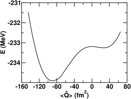
Figure 4: ²⁸Si potential energy landscape obtained in the absence of pairing with the SLy4 interaction.

The energy landscape of ²⁸Si calculated using ev8 with a constraining mass quadrupole field is shown in Fig. 4. Qualitatively, the landscape is very similar to that found for the USD interaction in Fig. 1. The ground state at the minimum of the curve has an oblate deformation with a value $\langle\hat{Q}\rangle=-89.2$ fm². This is larger than the value found for the USD interaction, which is to be expected because the USD is a defined in a restricted space. There are two other stationary points in the landscape, namely the spherical saddle point and and a shallow prolate minimum at $\langle\hat{Q}\rangle\approx 30$ fm². The deformation energy of the oblate solution $E_{\rm def}=E_{\rm mf}-E_{\rm sph}\approx 1.71$ MeV is lower than the deformation energy found for the USD interaction.

A standard spherical basis $|jm\rangle$ is constructed as described in Section IV. The reduced matrix elements of the mass quadrupole operator $\hat{Q}$ in the spherical basis are then extracted from

$$\!(j||\hat{Q}||j^{\prime})={5\over\sqrt{2j+1}}\sum_{m}(2\;0\;j^{\prime}m|jm)\langle jm|\hat{Q}|j^{\prime}m\rangle\;.$$ (18)

It is interesting to compare the reduced matrix elements (18) to those of the simple spherical Woods-Saxon (WS) model, taking the parameters of the Woods-Saxon plus spin-orbit potential from Bohr and Mottelson bm69 . Fig. 5 shows the ratio $|(j||\hat{Q}||j^{\prime})_{\rm SLy4}/(j||\hat{Q}||j^{\prime})_{\rm WS}|$ of the quadrupole reduced matrix elements in the Sly4 SCMF and in the WS model versus $|(j||\hat{Q}||j^{\prime})_{\rm WS}|$. We only show results for the valence $sd$ shell composed of the $0d_{5/2},1s_{1/2}$ and $0d_{3/2}$ orbitals. The solid circles correspond to diagonal elements ($j=j^{\prime}$) and open triangles to off-diagonal elements. The values of this ratio vary in the range $\sim 0.95-1.1$ (dotted lines in Fig. 5). Thus, quadrupole renormalization effects in shell-model calculations are more influenced by the truncation than by the particular treatment of the spherical mean field. Let us next examine those truncation effects.

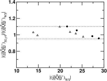
Figure 5: Ratio $|(j||\hat{Q}||j^{\prime})_{\rm SLy4}/(j||\hat{Q}||j^{\prime})_{\rm WS}|$ of the mass quadrupole reduced matrix elements in ²⁸Si versus $|(j||\hat{Q}||j^{\prime})_{\rm WS}|$. Solid circles: diagonal elements, open triangles: off-diagonal elements.

V.1 Truncation effects and operator rescaling

As mentioned earlier, the transformation from the deformed mean-field orbitals to the spherical basis is not unitary owing to truncation effects. The severity of the truncation can be assessed in several ways. The first is the trace of the truncated single-particle density matrix, Eq. (5), which should equal the number of particles in the truncated theory. With the truncation excluding orbitals beyond the $N,Z=20$ shell closures, we find the number of particles to be $27.75$ compared to $28$ for the full density matrix. When truncated to the valence $sd$ shell (i.e., without including the $0s_{1/2},0p_{3/2}$ and $0p_{1/2}$ core orbitals), the trace of the density matrix is 11.89 compared to $12$ valence particles in an $sd$ shell-model theory. A more severe test of the truncated single-particle density matrix is Eq. (6), requiring that its eigenvalues be zero or one. Thus we diagonalize the truncated proton and neutron density matrices and examine the eigenvalues. For the truncation to the 12+12 orbits of the $sd$ shell, we find that all eigenvalues are within 1.5% of the required values. We conclude that the projected density $\bf P{\boldsymbol{\rho}}_{\rm mf}P$ satisfies to a good accuracy the HF condition for a Slater determinant.

While the particle number is rather robust to truncation, the same is not true of the matrix elements of the quadrupole operator. To see how the effect of truncation evolves, we impose an upper cutoff energy on the spherical orbitals and examine how the quadrupole moment changes with this cutoff. This is shown in Fig. 6, describing $|\langle\hat{Q}\rangle|$ as a function of the maximal single-particle energy used to define the spherical model space. With a cutoff of +15 MeV unbound orbital energy, the quadrupole moment is reduced from its full value of -89 fm² by about 7%. Excluding all positive energy orbitals, the moment is -69 fm², a reduction of $\sim 25\%$. The truncation that excludes all orbitals above the $N,Z=20$ shell closure yields $\langle\hat{Q}\rangle=-54.4$ fm². Finally, we find a slightly lower value of $\langle\hat{Q}\rangle=-52.4$ fm² when truncating to the valence $sd$ shell. Thus, within a shell-model theory in the truncated valence $sd$ shell, the quadrupole operator should be rescaled by $89.4/52.4\approx 1.71$.

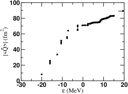
Figure 6: Quadrupole moment of the SCMF ground state of ²⁸Si using the SLy4 Skyrme energy functional and different truncations in the spherical basis. The horizontal axis is the maximum single-particle energy in the truncated space. Each solid circle corresponds to a spherical single-particle state of protons or neutrons. The untruncated moment of -89.2 fm² is shown by the arrow on the right.

V.2 Mapped Hamiltonian

To obtain the mapped Hamiltonian, we first calculate the transformation matrix $\bf U$ between the deformed and spherical bases, using the output orbital wave functions from ev8. We then find the deformed single-particle density matrix Eq. (3) and single-particle Hamiltonian Eq. (7) in the spherical basis. Next, we perform the multipole decomposition of the single-particle Hamiltonian ${\bf h}={\bf h}^{(0)}+{\bf h}^{(2)}$ using (8) and the Wigner-Eckart theorem (to convert the reduced matrix elements to matrix elements) to extract effective spherical shell orbital energies $\epsilon^{(0)}_{j}$ (see Eq. (9)) and and an effective quadrupole field ${\bf h}^{(2)}$. From this point on the procedure is identical to what we did for the USD Hamiltonian. We construct the effective CISM Hamiltonian (11) with a coupling constant $g$. A crude estimate for $g$ in the Hartree approximation is $g\approx-1/\langle\hat{h}^{2}_{0}\rangle=0.046$ MeV/fm⁴. To determine $g$ more precisely we match the deformation energy of the effective CISM Hamiltonian (11) to its value $1.71$ MeV found in the SCMF theory (of SLy4). The deformation energy of the CISM Hamiltonian for a given value of $g$ is calculated from the spherical and deformed (oblate) solutions of (11) in the HF approximation. This procedure gives us $g=0.0594$ MeV/fm⁴.

The mapped Hamiltonian can be tested by solving it in the HF approximation and comparing with the SCMF. The deformation energy is the same by construction. We obtain a quadrupole moment of $-55$ fm², which is $\sim 5\%$ larger than the SCMF quadrupole moment (projected on the $sd$ shell). We also find the spherical occupations of the deformed HF ground state of the CISM Hamiltonian to be rather close to the spherical occupations of the deformed SCMF minimum (see Table IV below).

V.3 Hartree approximation

In the previous section, we solved the CISM Hamiltonian in the HF approximation, i.e. including exchange. In this section we briefly examine the simpler Hartree approximation, because it allows some insight into the parametric sensitivities. Neglecting the exchange interaction, the dependence of the deformation energy $E_{\rm def}$ on the strength parameter $g$ can be conveniently determined in two steps. As a first step, the single-particle Hamiltonian

$${\bf h}_{\rm eff}={\bf h}^{(0)}+\xi{\bf h}^{(2)}_{0}$$ (19)

is solved as function of a coupling parameter $\xi$, say in the range $0<\xi<2$. One needs to keep the expectation values of ${\hat{h}}^{(0)}$ and ${\hat{h}}^{(2)}_{0}$ as a function of $\xi$, calculated with the ground-state density matrix $\rho_{\xi}$ of (19). For the second step, one determines the ground-state energy $E(g)$ by finding the minimum in

$$E(g)={\rm min}_{\xi}\left(\langle\hat{h}^{(0)}\rangle_{\xi}-{1\over 2}g{\langle\hat{h}^{(2)}_{0}\rangle}^{2}_{\xi}\right)\;.$$ (20)

The minimization in Eq. (20) with respect to $\xi$ is equivalent to the self-consistent condition $g\langle\hat{h}^{(2)}_{0}\rangle_{\xi}=\xi$. The deformation energy is then given by

$$E_{\rm def}(g)=E(0)-E(g)$$ (21)

Fig. 7 shows $\langle\hat{h}^{(0)}\rangle_{\xi}$ (left panel) and $\langle\hat{h}^{(2)}_{0}\rangle_{\xi}$ (right panel) versus $\xi$. The value of $\xi$ that minimizes the Hartree energy is determined through the competition between the two terms in Eq. (20).

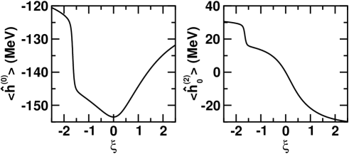
Figure 7: Left: $\langle\hat{h}^{(0)}\rangle_{\xi}$ versus $\xi$ in ²⁸Si. Right: $\langle\hat{h}^{(2)}_{0}\rangle_{\xi}$ versus $\xi$. The density matrix ${\boldsymbol{\rho}}_{\xi}$ corresponds to the single-particle (Hartree) Hamiltonian ${\bf h}_{\rm eff}={\bf h}^{(0)}+\xi{\bf h}^{(2)}_{0}$.

Performing next the minimization to get $E(g)$, we find the deformation energy curve shown in the left panel of Fig. 8. The panel on the right in Fig. 8 shows the quadrupole moment of the solution as a function of $g$. The discontinuity of $\langle\hat{Q}\rangle$ at $g\approx 0.037$ MeV^-1 describes a first order spherical to deformed shape transition. Note that the deformation energy $E_{\rm def}(g)$ in the deformed phase is a steep function of $g$; thus $g$ is well constrained by the fitting procedure. The solid triangles in Fig. 8 indicate the SLy4 SCMF point (in which the value of $g=0.0466$ MeV^-1 is fitted to give the correct deformation energy).

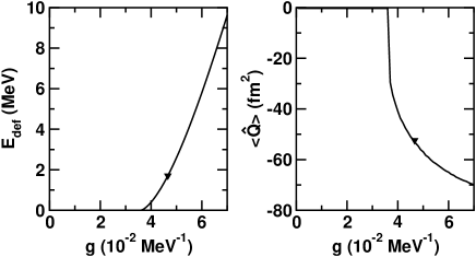
Figure 8: Left: deformation energy versus coupling parameter $g$ in ²⁸Si when solving the effective Hamiltonian (11) in the Hartree approximation. Right: quadrupole moment $\langle\hat{Q}\rangle$ versus $g$ in the Hartree approximation using the same effective Hamiltonian. The solid triangles describe the SCMF solution of the SLy4 energy functional (note that the triangle in the left panel is a fit).

The Hartree deformation energy $E_{\rm def}$ versus $\langle\hat{Q}\rangle$ in the truncated $sd$ space is plotted in Fig. 9. The solid triangle is the SLy4 SCMF point. It lies very close to the curve extracted from the effective Hamiltonian, showing that the effective theory closely reproduces the quadrupole moment in the truncated space.

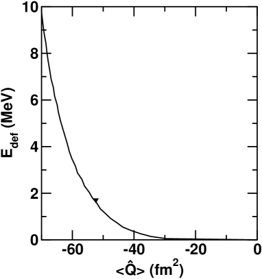
Figure 9: Deformation energy versus quadrupole moment of ²⁸Si using the Hartree approximation for the effective Hamiltonian (11) in the $sd$-shell. The triangle shows the SCMF solution for the SLy4 energy functional where the quadrupole moment is calculated in the truncated space ($sd$ shell).

V.4 Correlation energy

With the mapped shell-model Hamiltonian in hand, we are now in a position to compute the correlation energy as defined in Eq. (15). The HF energy of (11) is found to be $E_{\rm mf}=-147.44$ MeV. The ground-state energy $E_{\rm gs}$ is calculated using the shell-model code oxbash, putting in the orbital single-particle energies and interaction matrix elements from the mapped Hamiltonian (11). We find $E_{\rm gs}=-153.93$ MeV. Anticipating calculations in much larger shell-model spaces, we have also computed $E_{\rm gs}$ with the SMMC. Taking $\beta=6$ MeV^-1 and a time slice of $\Delta\beta=1/32$ MeV^-1 we find (using a stabilization method for the one-body propagation) $E_{\rm gs}=-153.87\pm 0.07$ MeV, in agreement with oxbash. For a time slice of $\Delta\beta=1/64$ MeV^-1 the SMMC result is $E_{\rm gs}=-153.94\pm 0.07$ MeV.

The quadrupolar correlation energy we find for ²⁸Si is then $E_{\rm corr}\approx-4.55$ MeV. This is quite comparable to the value we obtained from a similar reduction of the USD Hamiltonian ($4.3$ MeV). This gives one some confidence that the quadrupole correlation energy has a magnitude of about 4-5 MeV in ²⁸Si. It is interesting to compare this with the quadrupole correlation energy obtained by a completely different approach, the generator coordinate method (GCM) ben05 . Using that method in a global study of correlation energies archive , the authors of Refs. be05 ; ben05 obtained a correlation energy of 4.9 MeV for ²⁸Si, which is somewhat larger. However, these calculations included a pairing interaction, which we have not treated here. In particular, the $J=0$ wave functions used as the GCM basis are projected from deformed states that are constructed in the presence of a delta pairing force.

VI Other $\bf sd$ shell nuclei in the SCMF

We have repeated the mapping discussed in Section V for the SCMF of all other deformed $N=Z$ nuclei in the $sd$ shell, i.e., for ²⁰Ne, ²⁴Mg  and ³⁶Ar  (³²S  is found to be spherical, just as for the USD interaction). The results are summarized in Tables II, III and IV (including results for ²⁸Si).

Truncation effects on the deformed SCMF density matrix are summarized in Table II. The eigenvalues and trace of the truncated density matrix ${\bf P{\boldsymbol{\rho}}_{\rm mf}P}$ (projected on the valence $sd$ shell) are listed separately for protons and neutrons (there are 6 positive $z$-signature eigenvalues for each type of nucleon). We see that the HF condition ${\boldsymbol{\rho}}^{2}={\boldsymbol{\rho}}$ holds to a rather good accuracy for all four nuclei (all eigenvalues are very close to either 1 or 0). The condition that the trace is given by the number of valence particles is also satisfied quite well.

Table 2: Eigenvalues and trace of the truncated density matrix ${\bf P{\boldsymbol{\rho}}_{\rm mf}P}$ in the SCMF theory of the SLy4 Skyrme energy functional. Shown are results for deformed $4N$ nuclei in the $sd$ shell (separately for protons and neutrons).

Nucleus				eigenvalues of ${\bf P{\boldsymbol{\rho}}_{\rm mf}P}$				${\rm tr}\,({\bf P{\boldsymbol{\rho}}_{\rm mf}P})$
20Ne	protons	0.974	0.003	9 $\cdot 10^{-6}$	0	-3 $\cdot 10^{-6}$	-6$\cdot 10^{-6}$	1.953
	neutrons	0.975	0.003	4$\cdot 10^{-6}$	0	-4 $\cdot 10^{-6}$	-6 $\cdot 10^{-6}$	1.955
24Mg	protons	0.977	0.975	0.006	5$\cdot 10^{-6}$	-2$\cdot 10^{-6}$	-8$\cdot 10^{-6}$	3.915
	neutrons	0.977	0.975	0.006	7$\cdot 10^{-6}$	-2$\cdot 10^{-6}$	-6$\cdot 10^{-6}$	3.916
28Si	protons	0.991	0.990	0.987	0.004	7$\cdot 10^{-6}$	-6$\cdot 10^{-6}$	5.944
	neutrons	0.991	0.991	0.987	0.004	2 $\cdot 10^{-6}$	-8$\cdot 10^{-6}$	5.945
36Ar	protons	0.999	0.998	0.997	0.995	0.993	0.001	9.966
	neutrons	0.999	0.998	0.997	0.995	0.994	0.001	9.966

Table 3: SCMF with the SLy4 Skyrme energy functional and the mapped Hamiltonian Eq. (11) for deformed $4N$ $sd$ shell nuclei. All energies are in MeV, $\langle\hat{Q}\rangle$ is in fm² and $g$ is in MeV$/$fm⁴

Nucleus	Interaction	$g$	$E_{\rm sph}$	$E_{\rm mf}$	$E_{\rm def}$	$\langle\hat{Q}\rangle$	$\langle\hat{Q}\rangle_{\rm mf}$	$E_{\rm corr}$
	SLy4		-151.83	-157.43	5.6	49.0	84.0
20Ne	$\hat{h}^{(2)}$	0.077	-30.17	-35.78	fit	48.7		2.39
	SLy4		-187.20	-195.92	8.73	59.6	111.9
24Mg	$\hat{h}^{(2)}$	0.0394	-79.29	-88.03	fit	60.6		3.50
	SLy4		-233.19	-234.90	1.71	-52.4	-89.2
28Si	$\hat{h}^{(2)}$	0.0594	-147.67	-149.38	fit	-55.0		4.55
	SLy4		-303.16	-305.43	2.27	-43.4	-74.7
36Ar	$\hat{h}^{(2)}$	0.117	-274.53	-276.79	fit	-42.7		1.42

Table 4: Spherical occupations $\langle\hat{n}_{j}\rangle$ for deformed $4N$ nuclei in the $sd$ shell. The SCMF occupations (computed for the SLy4 Skyrme energy functional) are compared with the occupations for the mapped Hamiltonian Eq. (11) both in the HF approximation and in shell-model calculations.

Nucleus	Interaction	$p$ $0d_{5/2}$	$p$ $1s_{1/2}$	$p$ $0d_{3/2}$	$n$ $0d_{5/2}$	$n$ $1s_{1/2}$	$n$ $0d_{3/2}$
	SLy4	1.481	0.376	0.096	1.486	0.374	0.095
20Ne	$\hat{h}^{(2)}$ (HF)	1.565	0.372	0.064	1.569	0.366	0.065
	$\hat{h}^{(2)}$ (CISM)	1.531	0.403	0.066	1.539	0.396	0.065
	SLy4	3.290	0.411	0.215	3.293	0.408	0.215
24Mg	$\hat{h}^{(2)}$ (HF)	3.398	0.346	0.256	3.399	0.344	0.257
	$\hat{h}^{(2)}$ (CISM)	3.356	0.329	0.315	3.360	0.327	0.313
	SLy4	4.956	0.723	0.265	4.965	0.717	0.263
28Si	$\hat{h}^{(2)}$ (HF)	4.929	0.712	0.359	4.939	0.702	0.359
	$\hat{h}^{(2)}$ (CISM)	5.011	0.633	0.356	5.010	0.633	0.357
	SLy4	5.919	1.751	2.297	5.921	1.758	2.287
36Ar	$\hat{h}^{(2)}$ (HF)	5.979	1.694	2.327	5.980	1.702	2.3185
	$\hat{h}^{(2)}$ (CISM)	5.971	1.662	2.367	5.971	1.668	2.361

Table III compares results for the SCMF with the SLy4 Skyrme force and for the HF of the mapped CISM Hamiltonian (11) with $g$ determined by matching the deformation energy of both theories. Shown are the spherical and mean-field total energies, deformation energy and the quadrupole moment $\langle\hat{Q}\rangle$ in the truncated $sd$ shell-model space. We observe that the quadrupole moment of the effective theory deviates by at most $5\%$ from its value in the SCMF (for ²⁸Si).

We also show in Table III the total SCMF quadrupole moment $\langle\hat{Q}\rangle_{\rm mf}$ calculated in the deformed HF ground-state. Comparing $\langle\hat{Q}\rangle_{\rm mf}$ with $\langle\hat{Q}\rangle$ in the truncated $sd$ shell, we estimate that in the CISM theory the quadrupole operator should be rescaled by $\approx 1.71,1.88,1.70$ and $1.71$ for ²⁰Ne,²⁴Mg,²⁸Si  and ³⁶Ar, respectively.

The correlation energies (calculated from Eq. (15) with $E_{\rm gs}$ found using oxbash) are shown in the last column of Table III. The values we find are quite reasonable. They are below the values cited in archive , but we have not yet included pairing in our effective theory.

Finally, in Table IV we compare the occupations of the spherical valence orbitals of the SLy4 SCMF theory with similar occupations obtained with the mapped Hamiltonian (11). The latter are calculated in the HF approximation as well as in the shell-model theory from the expectation values of $\hat{n}_{j}=\sum_{m}\hat{a}^{\dagger}_{jm}\hat{a}_{jm}$ in the correlated CISM ground state.

VII The $Q\cdot Q$ interaction

In nuclear physics there is a long history of modeling the effective interaction as a quadrupole-quadrupole interaction of the form $\hat{Q}\cdot\hat{Q}$, including Elliott’s SU(3) model el58 and the pairing-plus-quadrupole model of Kisslinger and Sorensen ki63 . Since it is possible in some contexts to exploit the properties of the quadrupole operator, it is of interest to see how well a quadrupole-quadrupole interaction performs in our context. Thus, we apply the Hamiltonian

$$\hat{H}=\hat{h}^{(0)}-{1\over 2}g\hat{Q}\cdot\hat{Q}\;.$$ (22)

in the truncated shell-model space with the matrix elements of $\hat{h}^{0}$ and the mass quadrupole operator $\hat{Q}$ determined by the appropriate mean-field theory. We follow the same procedure we used before to determine the coupling constant $g$.

We have determined such an effective $\hat{Q}\cdot\hat{Q}$ interaction for the deformed $4N$ $sd$ shell nuclei ²⁰Ne, ²⁴Mg, ²⁸Si and ³⁶Ar , using the HF approximation of the USD interaction as the SCMF theory. We observe that the quadrupole moments calculated with both effective interactions (11) and (22) are quite close to the USD results. This can be seen in Fig. 10, where $\langle\hat{Q}\rangle$ (in fm²) is plotted versus mass number $A$. Results for the $\hat{Q}\cdot\hat{Q}$ interaction (solid triangles) and the interaction with $\hat{h}^{(2)}$ (solid squares) are compared with the USD results (open circles). The effective Hamiltonians (11) and (22) also yield similar occupations $\langle\hat{n}_{j}\rangle$ (see Fig. 2) and correlations energies (see Fig. 3).

Figure 10: Quadrupole moment in the SCMF method versus mass number $A$ for $4N$ $sd$-shell nuclei. Results are shown for two effective CISM Hamiltonians: the $\hat{Q}\cdot\hat{Q}$ interaction (22) (solid triangles) and the $\hat{h}^{(2)}\cdot\hat{h}^{(2)}$ interaction (11) (solid squares). They are compared with results for the USD Hamiltonian (open circles).

VIII Prospects and Conclusions

We are encouraged by the results we found for constructing a isoscalar quadrupolar interaction from the SCMF in the $sd$-shell, but much remains to be done to demonstrate that the method will be useful in deriving a global theory of correlation energies. We list some of the major tasks that should be addressed:

• So far, we have carried out the mapping only for nuclei that have deformed HF ground states. If the lowest-energy mean-field solution is spherical, we can use a constraining quadrupole field $\lambda\hat{Q}$ to deform the HF ground state and use this deformed solution to construct the effective CISM Hamiltonian. In particular, for a given strength $\lambda$ of the field, we can compare the deformation energy of the constrained SCMF theory with the deformation energy of the effective Hamiltonian in the constrained HF approximation. The Hartree-Fock Hamiltonian (14) of the effective CISM Hamiltonian is now replaced by

  $$h^{\lambda}_{ac}=h^{(0)}_{ac}-g\sum_{M}(-)^{M}h^{(2)}_{M;ac}\left(\sum_{bd}h^{(2)}_{-M;bd}\rho^{\lambda}_{db}\right)$$

  $$+g\sum_{M}(-)^{M}\sum_{bd}h^{(2)}_{M;ad}h^{(2)}_{-M;bc}\rho^{\lambda}_{db}+\lambda Q_{ac}\;,$$ (23)

  where $\rho^{\lambda}_{ac}$ is the self-consistent density matrix in the spherical basis (here $a=(jm)$) and $\hat{Q}$ is the axial quadrupole operator. A practical problem is how large should we take $\lambda$ to be. One possibility is to use the value of $\lambda$ that gives the deformed $J=0$ minimum.

• The real challenge of a global theory is the heavy, open-shell nuclei, and we should ask whether any severe problems will arise when we attempt to map the SCMF onto the CISM Hamiltonian. As a concrete example, consider the nucleus ¹⁶²Dy. It is strongly deformed, having an intrinsic quadrupole moment around 18 bn. The SCMF using the SLy4 interaction reproduces this value very well ben05 . The deformation energy when pairing is not included is quite large (about $20$ MeV). The $J=0$ projection and quadrupole fluctuations (in the presence of a delta pairing force) contribute an additional correlation energy of $\approx 3.4$ MeV archive .

  To use an CISM Hamiltonian to calculate deformation and correlation energies, one would need to truncate to a basis of the full shells, i.e., $N=82-126$ for neutrons and $Z=50-82$ for protons plus possibly some intruder states. Thus, a first test would be to see how well the consistency conditions Eqs. (5) and (6) are satisfied in such a truncated space.

  The next question that arises is the practicality of various implementations of the CISM Hamiltonian for solving in such large spaces. There are several approaches that have promise, including the shell model Monte Carlo (SMMC) method or94 ; al94 ; na97 , the Monte Carlo shell model ot99 and direct matrix methods such as those used by the Strasbourg group ca03 . One could also consider more approximate theories of the correlation energy, such as the RPA st02 .

• The mapping should be extended to include all other parts of the interaction that we believe are well-determined in the SCMF, in particular the interaction in the isovector monopole and quadrupole densities. This should be straightforward to carry out, requiring only that nuclei with $N\neq Z$ be considered in a more general parameterization of the interaction.

• The pairing interaction is very important in nuclear structure but is notoriously difficult to specify in detail, i.e., its density dependence and its spatial range (or equivalently the orbital space energy cutoff). Most SCMF energy functionals include a pairing interaction, but only an overall strength can be reliably determined in phenomenological theories. Thus, absent an ab initio theory of the pairing interaction, we cannot expect to have a reliable decomposition of the pairing fields in the mean-field Hamiltonian. Still, it should be possible to determine a strength parameter controlling the overall magnitude of pairing effects. Note that in the presence of pairing, the single-particle density matrices of the SCMF theory have the BCS form. Thus, to determine the parameters in the mapped Hamiltonian, one would use the HFB or the HF-BCS approximations for the self-consistent mean-field theory.

• An unsatisfactory aspect of our mapping is the lack of unitary of the transformation from the deformed basis to the truncated spherical basis. It would be useful to investigate mapping formalisms that yield density matrices that satisfy exactly the criteria we have discussed, i.e., Eqs. (5) and (6).

Despite this long list of tasks to be done, we believe that the method discussed here can be developed to produce a well-justified global theory of shell-model correlation energies, starting from a global SCMF theory (e.g., a Skyrme energy functional). Particularly encouraging is the finding that quadrupole correlations account for more than half the correlation energy in $sd$ shell nuclei.

Appendix: wave functions and matrix elements in the $z$-signature representation

A deformed single-particle wave function in the density functional theory is a two-component complex spinor $\psi=\left(\psi_{+}\atop\psi_{-}\right)$, or alternatively a four-component real spinor $\psi=\left({{{\psi_{1}\atop\psi_{2}}\atop\psi_{3}}\atop\psi_{4}}\right)$ with $\psi_{1}={\rm Re\,}\psi_{+}\;;\psi_{2}={\rm Im\,}\psi_{+}\;;\psi_{3}={\rm Re\,}\psi_{-}$ and $\psi_{4}={\rm Im\,}\psi_{-}$. The SCMF orbitals are chosen to have good parity $\pi$ and good $z$-signature bo85 . Such states have well-defined symmetry properties under each the three plane reflections $x\to-x;\;y\to-y;\;z\to-z$ (see Table 1 in Ref. bo85 ). Therefore it is sufficient to store their values in one octant (e.g., $x,y,z>0$).

The scalar product of two spinors $\psi$ and $\phi$ is a complex number with ${\rm Re\,}(\psi^{\dagger}\phi)=\sum_{i}\psi_{i}\phi_{i}$ and ${\rm Im\,}(\psi^{\dagger}\phi)=\psi_{1}\phi_{2}-\psi_{2}\phi_{1}+\psi_{3}\phi_{4}-\psi_{4}\phi_{3}$.

The find a standard basis of spherical single-particle orbitals $|jm\rangle$, it is necessary to calculate matrix elements of the quadrupole operators $\hat{Q}^{(2)}_{\mu}$ (see Section IV). We denote the $j+1/2$ orbitals with good $j$ and positive $z$-signature by $|ja\rangle$. The quadrupole matrix elements are obviously real and given by

$$\langle ja|\hat{Q}^{(2)}_{0}|jb\rangle=8\int_{x,y,z>0}dx\,dy\,dz\,(2z^{2}-x^{2}-y^{2})\,{\rm Re\,}(\psi^{\dagger}\phi)\;,$$ (24)

where $\psi$ and $\phi$ are the spinors describing $|ja\rangle$ and $|jb\rangle$, respectively.

To calculate $\langle ja|\hat{Q}^{(2)}_{\pm 1}|j\bar{b}\rangle$ we use the symmetry properties of the orbitals under plane reflections and find

$$\langle ja|xz|j\bar{b}\rangle = 8\int_{x,y,z>0}dx\,dy\,dz\,xz\,{\rm Re\,}(\psi^{\dagger}\bar{\phi})$$

$$\langle ja|yz|j\bar{b}\rangle = 8i\int_{x,y,z>0}dx\,dy\,dz\,yz\,{\rm Im\,}(\psi^{\dagger}\bar{\phi})\;,$$ (25)

Since the time-reversed spinor of $\phi$ is given by $\bar{\phi}=\left(\,\,\,\phi^{*}_{-}\atop-\phi^{*}_{+}\right)=\left({{{\,\,\,\phi_{3}\atop-\phi_{4}}\atop-\phi_{1}}\atop\,\,\phi_{2}}\right)$, we have

$${\rm Re\,}(\psi^{\dagger}\bar{\phi}) = \psi_{1}\phi_{3}-\psi_{3}\phi_{1}+\psi_{4}\phi_{2}-\psi_{2}\phi_{4}$$

$${\rm Im\,}(\psi^{\dagger}\bar{\phi}) = \psi_{3}\phi_{2}-\psi_{2}\phi_{3}+\psi_{4}\phi_{1}-\psi_{1}\phi_{4}\;.$$ (26)

The matrix elements of $\hat{Q}^{(2)}_{\pm 1}$ are calculated from (Appendix: wave functions and matrix elements in the $z$-signature representation) using $\hat{Q}^{(2)}_{\pm 1}=\mp\sqrt{6}\sum_{i}(x_{i}z_{i}\pm iy_{i}z_{i})$ (they are all real).

References

- (1) For a review see M. Bender, and P.H. Heenen and P.G. Reinhard, Rev. Mod. Phys. 75 121 (2003).
- (2) P. Hohenberg and W. Kohn, Phys. Rev. 136, B 864 (1964); W. Kohn and L.J. Sham, Phys. Rev. 140, A 1133 (1965).
- (3) For a review see B.A. Brown and B.H. Wildenthal, Annul. Rev. Nucl. Part. Sci. 38, 29 (1988).
- (4) B.A. Brown and W.A. Richter, Phys. Rev. C 58, 2099 (1998).
- (5) F. Tondeur, S. Goriely, J. M. Pearson, M. Onsi, Phys. Rev. C 62, 024308 (2000).
- (6) H. Nakada and Y. Alhassid, Phys. Rev. Lett. 79, 2939 (1997).
- (7) Y. Alhassid, S. Liu, and H. Nakada, Phys. Rev. Lett. 83, 4265 (1999).
- (8) Y. Alhassid, G.F. Bertsch, and L. Fang, Phys. Rev. C 68, 044322 (2003).
- (9) Y. Alhassid, D. J. Dean, S. E. Koonin, G. H. Lang, and W. E. Ormand, Phys. Rev. Lett. 72, 613 (1994).
- (10) B.H. Wildenthal, Progress Particle Nuclear Physics 11 5 (1984).
- (11) M.V. Stoitsov, J. Dobaczewski, W. Nazarewicz, and P. Ring, Computer Physics Communications 167 43 (2005).
- (12) P.-H. Heenen, to be published.
- (13) P. Bonche, H. Flocard, P.-H. Heenan, S.J. Krieger, and M.S. Weiss, Nucl. Phys. A 443, 39 (1985).
- (14) E. Chabanat, P. Bonche, P. Haensel, J. Meyer, and R. Schaeffer, Nucl. Phys. A 635, 231 (1998); Nucl. Phys. A 643, 441(E) (1998).
- (15) G.F. Bertsch, B. Sabbey, M. Uusn\a”nkki, Phys. Rev. C 71, 054311 (2005).
- (16) M. Bender, G.F. Bertsch, P.-H. Heenen, nucl-th/0508052 (2005).
- (17) A. Bohr and B. Mottelson, Nuclear Structure, Vol. 1 (Benjamin, NY, 1969), Eqs. (2-182) and (2-B9).
- (18) M. Bender, G.F. Bertsch, P.-H. Heenen, Phys. Rev. Lett. 94, 102503 (2005).
-
(19)
A table of correlation energies calculated in Ref. ben05
is available at
http://gene.phys.washington.edu/ev8/
correlation_energies.dat - (20) J.P. Elloitt, Proc. Roy. Soc. (London) A245 128,562(1958).
- (21) L. Kisslinger and R. Sorensen, Rev. Mod. Phys. 35 853 (1963).
- (22) W.E Ormand, D.J. Dean, C.W. Johson, G.H. Lang, and S.E. Koonin, Phys. Rev. C 49 1422 (1994).
- (23) T. Otsuka, T. Mizusaki, and M. Honma, J. Phys. G 25 699 (1999).
- (24) E. Caurier, M. Rejmund, and H. Grawe Phys. Rev. C 67 054310 (2003).
- (25) I. Stetcu and C. W. Johnson, Phys. Rev. C 66 034301 (2002).