FZJ–IKP(TH)–2005–32
Insights on scalar mesons from their radiative decays

Abstract

We estimate the rates for radiative transitions of the lightest scalar mesons $f_{0}(980)$ and $a_{0}(980)$ to the vector mesons $\rho$ and $\omega$. We argue that measurements of the radiative decays of those scalar mesons can provide important new information on their structure.

1 Introduction

Although studied since many decades, the lightest scalar mesons and, especially the $f_{0}(980)$ and $a_{0}(980)$, are still subject of debate regarding their fundamental structure. For example, these two mesons could be viewed as natural candidates for the genuine $1^{3}P_{0}$ $q\bar{q}$ states predicted by the standard quark models [1]. However, due to the proximity of these states to the $K\bar{K}$ threshold, a significant if not dominant $qq\bar{q}\bar{q}$ configuration is expected from a phenomenological point of view. Thus, it was argued (see, e.g., Ref. [2]) that the genuine $q\bar{q}$ ${}^{3}P_{0}$ nonet could be somewhere near $1.5$ GeV, while the states around $1$ GeV are due to a strong $S$-wave attraction between the two quarks and two antiquarks.

In such a scenario the $f_{0}(980)$ and $a_{0}(980)$ mesons could be realized either in form of compact $qq\bar{q}\bar{q}$ states [3, 4] or in form of loosely bound $K\bar{K}$ states. To complicate things further, within the latter picture there are even two possibilites regarding the nature of those scalar resonances, which are connected with the question whether there are sufficiently strong $t$–channel forces so that $K\bar{K}$ molecules are formed, as advocated in Refs. [5, 6, 7, 8], or whether the meson–meson interaction is dominated by s–channel states. In the former case the $f_{0}(980)$ and $a_{0}(980)$ would be purely composite particles, whereas in the latter case they would contain both elementary states and composite-particle components. For a much more thorough discussion on that issue and an overview of the extensive literature we refer the reader to the reviews in Refs. [9, 10, 11, 12, 13, 14].

Over the years many experiments have been proposed in order to distinguish among those scenarios, however, so far the smoking gun experiment has not been identified yet. For example, about a decade ago it was believed that data on the decays $J/\Psi\to\phi\pi\pi/\phi KK$ would allow to resolve the puzzle of the scalar mesons [15]. Even earlier Achasov and Ivanchenko had argued that measurements of the radiative decays of the $\phi(1020)$ to scalar mesons would provide decisive information on the structure of these long–debated objects [16]. The authors of that work demonstrated that the spectrum of, e.g., $\pi^{0}\pi^{0}$ in the reaction $\phi\to\gamma S\to\gamma\pi^{0}\pi^{0}$ would look drastically different in the presence or absence of a significant $K\bar{K}$ contribution, due to the proximity of both the mass of the scalar meson $S$ and that of the $\phi$ to the $K\bar{K}$ threshold. And indeed, the data [17, 18, 19] unambiguously show a prominent $K\bar{K}$ contribution. Based on large–$N_{C}$ considerations, this was interpreted then as a proof for a compact four–quark nature of the scalar mesons [20]. However, it is not clear a priori how quantitative the large–$N_{C}$ counting rules are in the scalar sector — for example, the large–$N_{C}$ analysis of the unitarised chiral perturbation theory amplitudes leads to large uncertainties for the $a_{0}/f_{0}(980)$ states [21]. After all, it is well known that, for the scalars, due to the presence of the nearby strong $S$-wave $K\bar{K}$ channel, unitarity corrections are large, as seen from the corresponding Flatté distributions [22, 23]. Thus, the large–$N_{C}$ picture might be obliterated. In particular, the admixture of a $K\bar{K}$ component in the scalar wave function should be large, as discussed in Refs. [5, 6, 24, 25].

For obvious reasons, a dominant role of the $K\bar{K}$ component in the $\phi\to\gamma S$ decays is naturally expected in the scenario where the scalar mesons are $K\bar{K}$ molecules. Thus, it might be not too surprising that explicit calculations utilizing such molecular models [26, 27, 8] were able to describe the spectrum of the radiative $\phi$ decays. Indeed, it was shown [28] recently on rather general grounds that, contrary to earlier claims [29, 30], the available experimental information is completely consistent with the molecular structure of the scalar mesons. We thus conclude that the radiative $\phi$ decays measure the molecular component of the scalar mesons. However, other observables are to be found that allow one to understand how much compact structure there is in addition.

There is a drawback of the radiative $\phi$ decays: beyond the prominence of the kaon loops, no further model–independent quantitative conclusion on the scalar mesons is possible because of the limited phase space available for these decays. In addition, gauge invariance forces the spectrum, for large pseudoscalar invariant masses, to behave as $\omega^{3}$, where $\omega$ denotes the photon energy. With the photon energy being just around $40$ MeV, only a small fraction of the spectral functions of the scalar mesons is visible in these reactions. As discussed in detail in Ref. [31], this causes uncertainties in the attempts to define the coupling constants and pole positions of the scalars.

In view of the difficulties outlined above, with the present paper, we would like to draw attention to another class of radiative decays — namely, to the radiative decays of the scalar mesons themselves. In particular, we want to provide evidence for the following properties of the reactions $S\to\gamma V$, where $S$ denotes the scalar mesons $a_{0}$ or $f_{0}$ and $V$ stands for the vector meson $\rho$ or $\omega$:

1. both quark loops and meson loops can be of equal importance;

2. there is significant phase space available for the final state;

3. since there is a sensitivity to the nonstrange contribution of the wave functions, a combined analysis of the $\phi$ radiative decays, as well as those of the scalars should help to map out the underlying quark structure of the latter.

Among those the first point is specifically interesting. It implies that, if the scalar mesons were predominantly $q\bar{q}$ or $qq\bar{q}\bar{q}$ states, then quark loops as well as meson loops should yield sizable contributions to the decay amplitude and, consequently, they should have a significantly larger decay rate to vector mesons as compared to $K\bar{K}$ molecules, where only meson ($K\bar{K}$) loops are present.

In this context we also consider the decay $S\to\gamma\gamma$ and show that, in this case, there is again a striking difference in the reaction mechanism in the sense that now the quark loops dominate while the meson loops are suppressed. As a consequence, there is a certain pattern or hierarchy in the studied radiative decay reactions involving scalar mesons ($\phi\to\gamma S$, $S\to\gamma V$, $S\to\gamma\gamma$) with characteristic differences for a compact ($q\bar{q}$ or $qq\bar{q}\bar{q}$) or molecular structure of those scalars. This suggests that a combined analysis of such decays, within a specific scenario of the scalar mesons, is actually a much more conclusive method to discriminate between these scenarios than just considering a single decay mode, like $\phi\to\gamma S$, as it happened in the past.

The paper is structured in the following way: In Sect. 2, we provide general expressions for the vertex function involving a photon, a scalar ($S$), and a vector ($V$) meson and for the total width of the transition $S\to\gamma V$. In Sect. 3, we consider different decay mechanisms for the scalar mesons, i.e., $q\bar{q}$ and $qq\bar{q}\bar{q}$ quark loops and meson loops, and we evaluate the decay width within the corresponding transition mechanisms. Sect. 4 is devoted to the decay of the scalar mesons to the $\gamma\gamma$ channel. Our results are analysed and discussed thoroughly in Sect. 5. The paper ends with a brief summary.

2 Some generalities

In order to write down the effective vertex for the $SV\gamma$ coupling, one is to respect gauge invariance for the photon. This is most easily implemented by using the field strength tensor for the latter. Therefore, the most general structure of the $SV\gamma$ vertex is

$$iW=M(p^{2},q^{2})[(k\cdot\epsilon^{V*})(q\cdot\epsilon^{\gamma*})-(\epsilon^{V*}\cdot\epsilon^{\gamma*})(k\cdot q)],$$ (1)

where $\epsilon^{V}_{\mu}$ and $\epsilon^{\gamma}_{\mu}$ are the polarisation vectors of the vector meson and photon, $q_{\mu}$ and $k_{\mu}$ are their four–momenta, respectively, and $p_{\mu}$ is the scalar four–momentum. For the $\phi$ radiative decays, the decay amplitude exhibits a strong $p^{2}$–dependence, due to the proximity of the $K\bar{K}$ threshold to both the $\phi$ mass as well as to the nominal mass of the scalar meson. However, for these decays, we have $q^{2}=m_{\phi}^{2}$, and thus it is not possible to investigate the $q^{2}$–dependence. On the other hand, for the decays $S\to\gamma V$ and the case of kaon loop contributions, $M(p^{2},q^{2})$ shows a significant dependence on both $p^{2}$ and $q^{2}$, due to the proximity of the $K\bar{K}$ threshold to the mass of the $a_{0}/f_{0}$ mesons and due to the finite width of the vector mesons, especially of the $\rho$–meson.

For stable scalar and vector mesons one could directly deduce the expression for the total width of the transition $S\to\gamma V$ from Eq. (1), which would be given by

$$\Gamma(m_{S}^{2})=\frac{m_{S}^{3}}{32\pi}|M(m_{S}^{2},m_{V}^{2})|^{2}\left(1-\left(\frac{m_{V}}{m_{S}}\right)^{2}\right)^{3},$$ (2)

with $m_{V}$ and $m_{S}$ being the nominal masses of the vector and scalar mesons. For the calculation of observables, in addition to the matrix element $M$, two more ingredients are relevant — namely, the propagator of the scalar meson $D_{S}(p^{2})$ and that of the vector meson, $D_{V}(q^{2})$. The latter modifies the invariant mass spectrum of the final state, cf. the detailed discussion in the appendix.

The finite width of the scalar mesons makes one study the decay rates as a function of the invariant mass of the decaying system. Consequently, in the total decay width, $D_{S}(m^{2}_{S})$ appears as a weight factor. For this distribution, one would need to use parametrizations given in the literature. Note that using such parametrizations one could run into complications connected to possible interference effects between the $f_{0}(980)$ and the broad $I=0$ $\pi\pi$ component usually referred to as “$\sigma$” [32]. In what follows we do not consider this possibility and give estimates for stable vectors and scalars.

As mentioned before, it is the transition matrix element $M$ which is the quantity of interest, and we investigate it now in more detail for various scenarios.

3 The transition matrix element $M$

In this section, we discuss the properties of $M$ in various models for the scalar mesons and for various mechanisms of the radiative decay.

3.1 Contribution of quark loops

Figure 1: Quark loop contribution to the radiative decay.

The simplest assignment for the $a_{0}(980)/f_{0}(980)$ mesons is the bound $q\bar{q}$ ${}^{3}P_{0}$ state [1]. Correspondingly, the radiative decay proceeds via a quark loop, as displayed at Fig. 1. If confinement is modeled by a quark–antiquark interaction, then the ingredients needed to calculate the transition matrix element are: i) the meson–quark–antiquark vertices, ii) the dressed propagators of quarks, and iii) the dressed photon–quark–quark vertex. Only if the underlying quark model provides these ingredients in a selfconsistent way, then the electromagnetic transition vertex is compatible with e.m. gauge invariance and the $SV\gamma$ transition amplitude takes the form of Eq. (1). Reliable calculations of the quark loop contributions can be done in the framework of the nonrelativistic quark model. The radiative transition ${}^{3}S_{1}(q\bar{q})\leftrightarrow{}^{3}P_{0}(q\bar{q})$ is an $E1$ transition, and the current in the rest frame of the initial meson $i$, in the lowest approximation, is

$${\mathbf{j}}_{i\to f}=\left\langle f\left|e_{q}\frac{{\mathbf{p}}_{q}}{m_{q}}\right|i\right\rangle+(q\leftrightarrow\bar{q}).$$ (3)

The expression for the matrix element $M$, extracted from Eq. (3), reads

$$M=\frac{2}{3}e\langle Q\rangle r_{if},$$ (4)

where

$$Q=\frac{1}{2}(Q_{q}-Q_{\bar{q}})$$ (5)

is the quark charge operator, and the radial part of the dipole matrix element between the initial and final states reads

$$r_{if}=\int r^{2}drR_{f}^{\dagger}(r)rR_{i}(r),$$ (6)

with $R_{i,f}(r)$ being the radial wave functions for the initial and the final states, respectively.

Generally, the decay rate for $E1$ transitions between the ${}^{3}S_{1}$ and ${}^{3}P_{J}$ states is given by (see, e.g., Ref. [33])

$$\Gamma=\frac{4(2J+1)}{27}\alpha\langle Q\rangle^{2}\omega^{3}r^{2}_{if},$$ (7)

for the ${}^{3}S_{1}\to^{3}P_{J}\gamma$ decays, and by

$$\Gamma=\frac{4}{9}\alpha\langle Q\rangle^{2}\omega^{3}r^{2}_{if}$$ (8)

for the ${}^{3}P_{J}\to^{3}S_{1}\gamma$ decays. Here $\omega$ stands for the photon energy and the charge factor is readily calculated for a given flavour of the initial and final states ($n$ denotes $u$ and/or $d$ quark):

$$\langle Q\rangle^{2}=\left\{\begin{array}[]{ccll}\frac{1}{36},&\rm for&n{\bar{n}}\to n{\bar{n}}&\rm with~{}the~{}same~{}isospin,\\ \frac{1}{4},&\rm for&n{\bar{n}}\to n{\bar{n}}&\rm with~{}different~{}isospins,\\ \frac{1}{9},&\rm for&s{\bar{s}}\to s{\bar{s}}.&\end{array}\right.$$ (9)

One might question the applicability of the nonrelativistic or the naively relativised quark model to the mentioned decays. Nevertheless, experimental data can be used to estimate the needed matrix element. We may use the known radiative decay rate of the bona fide quarkonium $f_{1}(1285)$ [34], as a genuine ${}^{3}P_{1}$ $q\bar{q}$ state made of light quarks:

$$\Gamma(f_{1}(1285))\to\gamma\rho)=1320\pm 312{\rm keV}.$$ (10)

As shown in Ref. [35], nonrelativistic quark models with standard parameters yield results for the decay $f_{1}(1285)\to\gamma\rho$ that are in good agreement with the data. To relate this matrix element to the ones of interest we assume $SU(6)$ symmetry for the wave functions which is expected to provide a reasonable order–of–magnitude estimate for the rates. In this case the values of the matrix elements $r_{if}$ are to be equal for all members of the $P$–multiplet.

Then one gets from Eqs. (7)-(10):

$$\begin{array}[]{l}\Gamma(a_{0}\to\gamma\omega)=\Gamma(f_{0}(n\bar{n})\to\gamma\rho)=125~{}{\rm keV},\\ \Gamma(a_{0}\to\gamma\rho)=\Gamma(f_{0}(n\bar{n})\to\gamma\omega)=14~{}{\rm keV},\\ \Gamma(f_{0}(s\bar{s})\to\gamma\omega)=31~{}{\rm keV}\times\sin^{2}\theta,\\ \Gamma(f_{0}(s\bar{s})\to\gamma\rho)=0,\\ \end{array}$$ (11)

where $\sin\theta$ measures the (small) $\phi-\omega$ mixing.

While the expressions (7) and (8) take apparently nonrelativistic form, relativistic corrections are actually included in these dipole formulae, provided the masses and the wave functions of the initial and final mesonic states are taken to be solutions of a quark–model Hamiltonian with relativistic corrections taken into account (see Refs. [36, 37] for a detailed discussion). With relativistic corrections to the wavefunctions taken into account the values of $r_{i}j$ for ${}^{3}P_{0}$ and $3^{P}_{1}$ states are not equal to each other anymore. So the estimates (11) are to be considered as order-of-magnitude ones.

Similarly we obtain for $\phi$ decay:

$$\begin{array}[]{l}\Gamma(\phi\to\gamma a_{0})=0.37~{}{\rm keV}\times\sin^{2}\theta,\\ \Gamma(\phi\to\gamma f_{0}(s\bar{s}))=0.18~{}{\rm keV},\\ \Gamma(\phi\to\gamma f_{0}(n\bar{n}))=0.04~{}{\rm keV}\times\sin^{2}\theta.\\ \end{array}$$ (12)

In this context let us mention that the pure $s\bar{s}$ assignment for $f_{0}$ seems implausible as it implies an OZI suppression of the $\pi\pi$ mode in the $\phi$ radiative decay, so that some mixing with an $n\bar{n}$ isoscalar state is needed to reproduce the branching fraction of the $f_{0}(980)$ to $\pi\pi$.

We would like to point out that the predictions for the decay width ratios of rates,

$$\begin{array}[]{c}\Gamma[(f_{0}(n\bar{n})\to\gamma\rho_{0}):(a_{0}\to\gamma\omega):(f_{0}(n\bar{n})\to\gamma\omega):(a_{0}\to\gamma\rho_{0})]=\\ 9:9:1:1,\end{array}$$ (13)

which are readily deduced from Eq. (11), are based only on the isospin relations (9) and are, therefore, robust.

3.2 Contributions of annihilation graphs for $qq\bar{q}\bar{q}$ scalars

Figure 2: Annihilation contributions to the radiative decay of $qq\bar{q}\bar{q}$ scalars.

In the diquark–antidiquark model [3, 4] both $f_{0}$ and $a_{0}$ can be identified with $sn\bar{s}\bar{n}$ states belonging to a cryptoexotic $\overline{3}\otimes 3$ flavour nonet,

$$f_{0}=\frac{1}{2}([su][\bar{s}\bar{u}]+[sd][\bar{s}\bar{d}]),$$

$$a_{0}(I_{3}=0)=\frac{1}{2}([su][\bar{s}\bar{u}]-[sd][\bar{s}\bar{d}]).$$

The radiative decays of the $qq\bar{q}\bar{q}$ states proceed via annihilation of a $q\bar{q}$ pair, as shown at Fig. 2. Thus, in the transition $S\to\gamma\rho/\omega$, the $s\bar{s}$ pair annihilates, so that one has

$$\frac{\Gamma(f_{0}\to\gamma\rho)}{\Gamma(f_{0}\to\gamma\omega)}=0,$$ (15)

while the $\phi-\omega$ mixing could generate small nonzero values of the ratio

$$\frac{\Gamma(a_{0}\to\gamma\omega)}{\Gamma(a_{0}\to\gamma\rho)}\sim\sin^{2}\theta.$$ (16)

On the contrary, the decay $\phi\to\gamma S$ with the four–quark scalars (LABEL:4q) proceeds via creation of a $n\bar{n}$ pair (if one neglects the $\phi-\omega$ mixing), yielding

$$\frac{\Gamma(\phi\to\gamma a_{0})}{\Gamma(\phi\to\gamma f_{0})}=9.$$ (17)

Note that the experimental value for this ratio is around 1/6 [35].

The assumption (LABEL:4q) is compatible with the $a_{0}/f_{0}$ mass degeneracy. However, with the $sn\bar{s}\bar{n}$ assignment for $f_{0}$, a superallowed decay to $\pi\pi$ is impossible, so that one is forced to assume a mixing of the isoscalar $sn\bar{s}\bar{n}$ state with a $\sigma$-like $nn\bar{n}\bar{n}$ state (see [4]). Note that there is no such problem for the superallowed decay $a_{0}\to\pi\eta$, since the $\eta$ contains an admixture of the strange quark pair.

There are no theoretical estimates of the absolute values for the $qq\bar{q}\bar{q}$ radiative decay rates. Moreover, since no single four–quark state is unambiguously identified, there is also no experimental anchor at our disposal, similar to Eq. (10), which could allow one to predict absolute values of these rates.

3.3 Contribution of meson loops

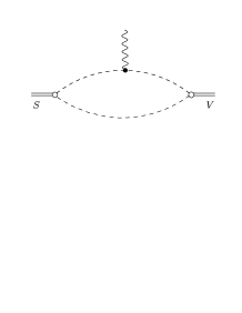
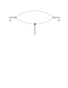
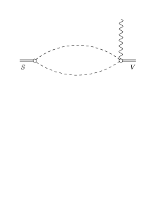
a)	b)	c)

Figure 3: Meson loop contributions to the radiative decay of scalar mesons. Diagram c) is required to provide the overall gauge invariance of the amplitude.

The contribution of meson loops is shown diagrammatically in Fig. 3, where the diagrams $a)$ and $b)$ correspond to the coupling of the photon to the charge of the intermediate pseudoscalar meson and the diagram $c)$ stems from gauging the decay vertex of the vector meson to two pseudoscalars. The explicit expressions for the corresponding matrix elements read

$$W_{a}=W_{b}=-eg_{S}g_{V}\int\frac{d^{4}l}{(2\pi)^{4}}\frac{\epsilon^{\gamma*}{\cdot}(p+q-2l)\;\epsilon^{V*}{\cdot}(2l+q)}{((p-l)^{2}-m_{P}^{2})((q-l)^{2}-m_{P}^{2})(l^{2}-m_{P}^{2})},$$

$$W_{c}=-2eg_{S}g_{V}(\epsilon^{\gamma*}{\cdot}\epsilon^{V*})\int\frac{d^{4}l}{(2\pi)^{4}}\frac{1}{((p-l)^{2}-m_{P}^{2})(l^{2}-m_{P}^{2})}.$$

Adding these three we get for the amplitude $M$ introduced in Eq. (1):

$$M(m_{V}^{2},m_{S}^{2})=\frac{eg_{S}g_{V}}{2\pi^{2}m_{P}^{2}}I(a,b),$$ (18)

where $a=\frac{m_{V}^{2}}{m_{P}^{2}}$, $b=\frac{m_{S}^{2}}{m_{P}^{2}}$, with $m_{P}$ being the mass of the pseudoscalar; $g_{S}$ and $g_{V}$ are the $SP^{+}P^{-}$ and $VP^{+}P^{-}$ coupling constants, while $I(a,b)$ is the loop integral function. An analytical expression for this function can be found, e.g., in Refs. [16, 29]. The dependence of $(a-b)^{2}|I(a,b)|^{2}$ on the mass of the scalar meson is shown in Fig. 4.

  

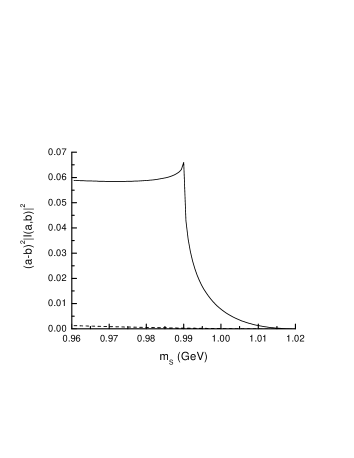
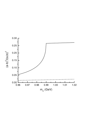
Figure 4: Dependence of the function $(a-b)^{2}|I(a,b)|^{2}$ on the mass of the scalar meson (in GeV) for the kaon loop (solid line) and for the pion loop (dashed line). Here $m_{V}=m_{\phi}$ for the left plot ($\phi$ decay), and $m_{V}=m_{\rho/\omega}$ for the right plot (scalar decay).

What pseudoscalars can be responsible for the transitions under consideration? The $a_{0}$ meson is known to couple to $\pi\eta$ and $K\bar{K}$, while $\rho$, $\omega$, and $\phi$ do not couple to $\pi\eta$. Thus, for the $a_{0}$, only the kaon loop is relevant. The $f_{0}$ meson couples to $\pi\pi$ and $K\bar{K}$, whereas the only vector meson coupling to $\pi\pi$ is the $\rho$ meson. Therefore, for the $f_{0}$, the pion loop could contribute together with the kaon loop. Nevertheless, the loop integral depends drastically on the relation between the initial and final meson masses and on the pseudoscalar threshold. For both cases of the $\phi\to\gamma a_{0}/f_{0}$ and $a_{0}/f_{0}\to\gamma\rho/\omega$ decays the contribution from the pion loop is small (see Fig. 4). Thus, in what follows, only the kaon loop mechanism is considered.

The only input needed to evaluate the kaon loop contribution to the radiative decays are the effective coupling constants $g_{S}$ and $g_{V}$. The decay constant for $\phi\to K^{+}K^{-}$ is readily calculated from the $\phi$ width,

$$\frac{g_{\phi KK}^{2}}{4\pi}\approx 1.77,$$ (19)

and the decay constants for $\rho/\omega\to K^{+}K^{-}$ can be estimated from that for the $\rho\to\pi\pi$ decay with the help of $SU(3)$ symmetry considerations yielding

$$g_{V}=g_{\rho K^{+}K^{-}}=g_{\omega K^{+}K^{-}}=\frac{1}{2}g_{\rho\pi\pi}\approx 2.13,\quad\frac{g_{V}^{2}}{4\pi}\approx 0.36.$$ (20)

The last missing ingredient is $g_{S}$. In Ref. [28] the value of

$$\frac{g_{S}^{2}}{4\pi}=16m_{K}\sqrt{\varepsilon m_{K}}=0.6\ \mbox{GeV}^{2}$$ (21)

was estimated. To come to this number the mass of 980 MeV for both scalars was used which corresponds to a binding energy of $\varepsilon=10$ MeV. The quoted estimate is based on assuming a stable molecule formed by a pointlike interaction in the $K\bar{K}$ channel and thus should be viewed as qualitative. Such a value of $g_{S}$ lies within the range given by various parametrisations of the $a_{0}/f_{0}$ propagators existing in the literature — see Tables in Refs. [22, 25].

Within the $q\bar{q}$ and the 4–quark pictures, relations between the effective couplings of the $a_{0}$ and $f_{0}$ to $K\bar{K}$ can be derived readily. In the $q\bar{q}$ picture, the scalar mesons are ${}^{3}P_{0}$ states and, for the flavour–independent strong interaction, one should have, approximately,

$$g_{f_{0}KK}=\left\{\begin{array}[]{ccl}g_{a_{0}KK},&\rm for&f_{0}(n\bar{n})\\ \sqrt{2}g_{a_{0}KK},&\rm for&f_{0}(s\bar{s}),\end{array}\right.$$ (22)

though one should keep in mind that effects like the instanton–induced forces or an admixture of the scalar glueball in the wave function of the $f_{0}$ may destroy these equalities.

In the four–quark model, the scalar decays are superallowed and one has, for the $a_{0}$ and $f_{0}$ with the quark content given by Eq. (LABEL:4q), the relation

$$g_{f_{0}KK}=g_{a_{0}KK},$$ (23)

which may be distorted by the aforementioned mixing of the isoscalar $sn\bar{s}\bar{n}$ with the $\sigma$-like state.

On the other hand, estimates for the absolute values of the scalar coupling constants $g_{S}$ involve calculations of strong decays of quark–antiquark, four–quark or molecular states, which are very model dependent. One might consider to rely on experimental data for determining the absolute values of $g_{S}$. However, the coupling constants extracted from data are afflicted with large uncertainties, i.e., they exhibit variations up to a factor of $2\div 3$ — see Tables in Refs. [22, 25]. This is due to the scaling property of the Flatté distributions near the $K\bar{K}$ threshold, as discussed in detail in Ref. [22]. In the following we use the value of Eq. (21) for the scalar coupling.

With the given values for the couplings one obtains, in the kaon loop model, the values

$$\Gamma(\phi\to\gamma S)=0.6~{}{\rm keV},$$ (24)

and

$$\Gamma(a_{0}/f_{0}\to\gamma\rho/\omega)=3.4~{}{\rm keV}.$$ (25)

One should keep in mind that the results (24) and (25) are obtained by assuming the scalar vertex to be pointlike. The procedure which allows one to include the effects of finite–range scalar meson formfactors in a gauge–invariant way is well known [8, 29, 30]. As shown in detail in [28], these corrections are small in the case of the $\phi\to\gamma a_{0}/f_{0}$ decay. The reason for this is the following: the $\phi$ as well as the $a_{0}/f_{0}$ are close to the $K\bar{K}$ threshold, and the loop integral is saturated by nonrelativistic values of the loop momentum, $|\vec{k}|\ll m_{K}$, where $m_{K}$ is the kaon mass. The range of the scalar formfactor is defined by the range of the force and, in the absence of pion exchange between kaons in the scalar sector, the latter is obviously larger than the kaon mass. On the contrary, the mass of the $\rho/\omega$ is significantly smaller than $2m_{K}$, and the typical values of the momentum in the loop integral are not that small. Thus, for the decays $S\to\gamma\rho/\omega$, one expects corrections due to the finite range of the scalar formfactor, which would reduce the pointlike result.

4 Comment on the $\gamma\gamma$ decays of scalar mesons

The transition $a_{0}/f_{0}\to\gamma\gamma$, closely related to the class of the reactions $S\to\gamma V$, probes the matrix element $M(p^{2},q^{2})$ in a kinematical regime quite different from the decays discussed above.

The $\gamma\gamma$ decay can proceed via the quark loop mechanism. Nonrelativistic quark model estimates give [38]

$$\Gamma_{\gamma\gamma}(^{3}P_{0})=\frac{15}{4}\Gamma_{\gamma\gamma}(^{3}P_{2})=432\alpha^{2}\langle Q^{2}\rangle^{2}\frac{|R^{\prime}(0)|^{2}}{M_{0}^{4}},$$ (26)

where $R(r)$ is the radial part of the wave function, and $M_{0}$ is the mass of the $P$-wave quark–antiquark state, which, in the leading nonrelativistic approximation, is supposed to be the same for all the members of the $P$-wave multiplet.

The calculation of the squared charge factors $\langle Q^{2}\rangle^{2}$ yields for the isospin ratios

$$\Gamma[(a_{0}\to\gamma\gamma):(f_{0}(n\bar{n})\to\gamma\gamma):(f_{0}(s\bar{s})\to\gamma\gamma)]=9:25:2.$$ (27)

Therefore, one can try to estimate the decay width for the scalar $f_{0}(980)$ from the width of the tensor $f_{2}(1270)$, which is known to be a good $n\bar{n}$ state. The PDG [34] quotes

$$\Gamma(f_{2}(1270)\to\gamma\gamma)=2.61\pm 0.30~{}{\rm keV},$$ (28)

that gives

$$\Gamma(f_{0}(980)\to\gamma\gamma)=\frac{15}{4}\left(\frac{M(f_{0})}{M(f_{2})}\right)^{3}\Gamma(f_{2}(1270)\to\gamma\gamma)=4.5~{}{\rm keV}.$$ (29)

Similar results were obtained in other computations of $\Gamma(f_{0}(980)\to\gamma\gamma)$ based on the $q\bar{q}$ model of the scalar mesons [39, 40].

In the $qq\bar{q}\bar{q}$ picture, the predictions appear to be of the order of $0.3$ keV for both the $f_{0}$ and the $a_{0}$ [41].

The $\gamma\gamma$ decay can also proceed via the kaon loop mechanism (see, e.g., Ref. [42]), with the matrix element given by Eq. (18) with $m_{V}^{2}=0$. For a pointlike scalar with the mass of $980$ MeV and $g_{S}^{2}/4\pi$ = 0.6 GeV² one obtains

$$\Gamma(S\to\gamma\gamma)\approx 0.24~{}{\rm keV}.$$ (30)

In line with the reasoning of the previous section, this value comes out as our prediction for the $\gamma\gamma$ decay of a molecule. However, in the kinematical regime of the $S\to\gamma\gamma$ transition, the momenta in the kaon loop are in the order of the kaon mass and, as in the case of the $S\to\gamma V$ transitions, one expects corrections due to the finite range of the form factor at the scalar vertex. Indeed an explicit calculation within a molecular model of the scalar mesons [43] yields results for the decay widths (0.20 keV for the $f_{0}$ and 0.78 keV for the $a_{0}$) that differ from our predictions, but are still in remarkable qualitative agreement with them given the simplicity of our approach.

The result of Eq. (30) as well as the applied technique is very different from those in Refs. [39, 44], where also the $\gamma\gamma$ width of scalar molecules was calculated. The authors obtain $\Gamma(f_{0}(K\bar{K})\to\gamma\gamma)=0.6~{}{\rm keV}$ [39] and $6$ keV [44]. In these references, similarly to the positronium $\gamma\gamma$ decay, the transition matrix element is taken proportional to the value of the $K\bar{K}$ wave function at the origin. Not only is this quantity model dependent (as reflected in the order of magnitude variation of the calculated widths), but also we suppose that the validity of such an approach is highly questionable for the considered decays: the range of the $K\bar{K}\to\gamma\gamma$ transition operator is of the same order as that of the wave function.

The experimental values for the $\gamma\gamma$ widths of scalars are [34]

$$\Gamma_{\gamma\gamma}(f_{0}(980))=0.39^{+0.10}_{-0.13}~{}{\rm keV},\quad\Gamma_{\gamma\gamma}(a_{0}(980))=0.30\pm 0.10~{}{\rm keV}.$$ (31)

The estimates based on the nonrelativistic quark loop (29) are in clear disagreement with these data. Although relativistic corrections to the formula (26) evaluated in Ref. [47] reduce the ratio $\Gamma_{\gamma\gamma}(^{3}P_{0})/\Gamma_{\gamma\gamma}(^{3}P_{2})$ by a factor of 2, this result is still much larger than the experimental values (31). On the other hand, the kaon loop mechanism estimate (30) is certainly compatible with them. Moreover, as shown recently in Ref. [45], the new data [46] for the reaction $\gamma\gamma\to\pi^{+}\pi^{-}$ in the vicinity of the $f_{0}(980)$ resonance can be described with the kaon loop mechanism using the weight factor $D_{S}(m^{2}_{S})$ which reproduces the $S$-wave $\pi\pi$ scattering data.

Concluding, one can say that the existing data on the $\gamma\gamma$ widths of scalars seems to favor a molecular structure of the $f_{0}/a_{0}$ mesons. However, one has to admit that, at present, no reliable estimation of the theoretical uncertainty involved in the value quoted in Eq. (30) can be given.

5 Discussion

The results of the previous sections are summarised in Fig. 5, where, for the sake of transparency, the relative contributions of the quark loop and kaon loop mechanisms are displayed for various kinematical regimes probed by the radiative decays involving scalar mesons.

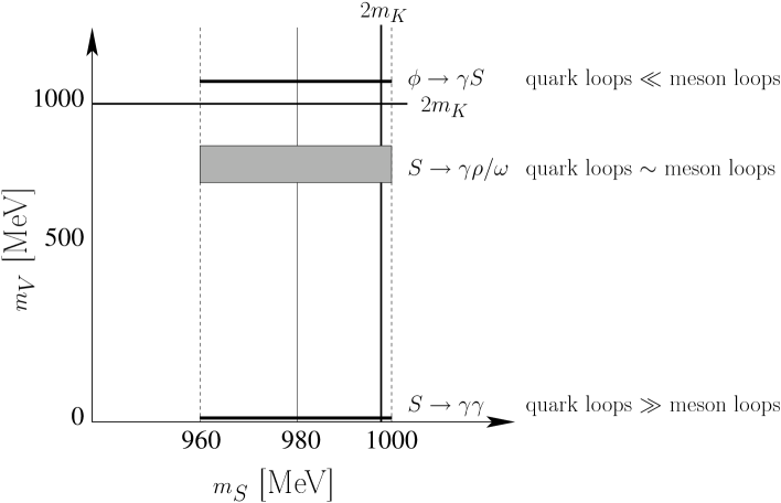
Figure 5: Illustration of various kinematical regimes probed by the decays involving scalars.

The message disclosed by this figure is quite clear: the closer the mass of the vector meson is to the $K\bar{K}$ threshold, the larger is the contribution of the kaon loop mechanism to the decay amplitude. Now recall that the quark loop mechanism is of relevance only if the scalars indeed carry a significant quark component, whereas the kaon loop mechanism contributes in both cases, i.e., in the $q\bar{q}$ (or $qq\bar{q}\bar{q}$) as well as in the $K\bar{K}$ molecule scenario. Thus, in order to discriminate between these two scenarios, it is most promising to study those decays where the quark loop mechanism, if present, is significant.

The data on $\phi$ radiative decays yield [34]:

$$\begin{array}[]{l}Br(\phi\to\gamma a_{0})\simeq 7.6\cdot 10^{-5},\quad\Gamma(\phi\to\gamma a_{0})\simeq 0.3~{}{\rm keV},\\ Br(\phi\to\gamma f_{0})\simeq 4.4\cdot 10^{-4},\quad\Gamma(\phi\to\gamma f_{0})\simeq 1.9~{}{\rm keV},\end{array}$$ (32)

indicating that the kaon loop mechanism indeed dominates the radiative transition $\phi\to\gamma S$. This can be understood from the proximity of both the mass of the $\phi$ and the mass of the scalar mesons to the $K\bar{K}$ threshold. The question that remains to be addressed is, however, how much room is there for an additional quark component. We argue that we can get a handle on this quark component of the scalar structure when looking at the decays $S\to\gamma\rho/\omega$, for there the kinematical situation is quite different. As seen from the estimates given by Eqs. (11) and (25), in those decays the quark loop and kaon loop mechanisms should yield contributions of the same order. Accordingly, for scalar mesons with a $q\bar{q}$ structure, where both mechanisms contribute, the radiative transition widths should be significantly larger than for $K\bar{K}$ molecules, where only the kaon loop mechanism can occur. Thus, the radiative decays $a_{0}/f_{0}\to\gamma\rho/\omega$ appear to be a much more decisive testing ground for discriminating between models for the scalar mesons than the radiative $\phi$ decays.

The estimates of the radiative decay widths of scalar mesons in various models are collected in Table 1. The numbers demonstrate that the $q\bar{q}$ component of the scalar mesons implies characteristic ratios for the radiative decays into isovector or isoscalar vector mesons, namely $\Gamma(a_{0}\to\gamma\rho)/\Gamma(a_{0}\to\gamma\omega)\approx 1/10$ and $\Gamma(f_{0}\to\gamma\rho)/\Gamma(f_{0}\to\gamma\omega)\approx 10$. This is in strong contrast to the corresponding ratios for the meson loop contributions (driven by the kaon loops), where all transitions are predicted to be of the same order of magnitude so that those ratios should be in the order of 1.

The latter point means that the scalar radiative transition is a filtering reaction. The quark loop mechanism “senses” the $q\bar{q}$ flavour, with the ratios of rates for different isospin content given by Eq. (13). Thus, one is able to measure the $q\bar{q}$ content of a specific scalar meson produced in a specific reaction simply by measuring the ratio of decay rates $(f_{0}\to\gamma\rho)/(f_{0}\to\gamma\omega)$ or $(a_{0}\to\gamma\omega)/(a_{0}\to\gamma\rho)$.

Decay mechanism	Process	Radiative width in keV
quark loop	$a_{0}\to\gamma\rho$	14
	$a_{0}\to\gamma\omega$	125
	$f_{0}(n\bar{n})\to\gamma\rho$	125
	$f_{0}(n\bar{n})\to\gamma\omega$	14
$K\bar{K}$ loop	$a_{0}/f_{0}\to\gamma\rho/\omega$	3

Table 1: Radiative $S\to\gamma\rho/\omega$ transition in various models.

Another advantage of the radiative scalar decays is related to the fact that the phase space available for the final state is not small, in contrast to the radiative decays of the $\phi$ meson. Thus, simultaneous studies of data on $\phi$ radiative decays and scalar radiative decays could be useful in establishing such fundamental characteristics of the scalar mesons as their pole positions and coupling constants. Indeed, the kaon loop mechanism is dominant in the $\phi$ radiative decay. The transition matrix element in the kaon loop mechanism exhibits a rather peculiar dependence on the masses of the initial and final mesons. The photon emitted in the $\phi$ radiative decay is relatively soft, $\omega\sim 40$ MeV, so that the corresponding matrix element decreases very rapidly in the upper part of the scalar–mass range, from the $K\bar{K}$ threshold to the mass of $\phi$ (see the first plot in Fig. 4). On the other hand, in the reaction $S\to\gamma\omega/\gamma\rho$, the photon energy appears to be large, about $200$ MeV, so that the matrix element exhibits a rather different pattern. In the quark loop model it is nearly constant. As far as the kaon loop mechanism is concerned, the corresponding matrix element decreases rapidly with the scalar invariant mass from the $K\bar{K}$ threshold downwards, but remains practically constant above the $K\bar{K}$ threshold (see the second plot in Fig. 4). In such a case it is then possible to analyse the upper part of the spectrum with much less uncertainty than in the $\phi$ radiative decay.

For the sake of completeness we would like to mention that the radiative decays of scalar mesons have been also studied within the Vector Dominance Model. Corresponding results can be found, e.g., in Ref. [48].

6 Summary

We have demonstrated that for radiative decays of the scalar mesons $f_{0}(980)$ and $a_{0}(980)$ to the vector mesons $\rho$ and $\omega$, meson loops and quark loops lead to very different predictions for the ratio of the decays to $\rho$ and $\omega$, respectively. Specifically, it follows from our results that for objects with a significant component from a compact quark state both types of loops should be equally significant. On the other hand, for scalar mesons that are $K\bar{K}$ molecules only meson loops can contribute. The inferred estimates for the decay rates and, in particular, the ratios that follow for the two scenarios are so drastically different that it should be possible to discriminate between them once experimental information becomes available.

We have also pointed out that the radiative decay rates involving the scalar mesons (such as $\phi\to\gamma S$, $S\to\gamma V$, and $S\to\gamma\gamma$) exhibit a distinct hierarchy pattern for a compact as well as for a molecular structure of the scalars. This pattern can be likewise used to distinguish between the two scenario, and, as an ultimate goal, to define the admixture of the bare confined state in the wave function of the scalar mesons. It requires, however, that a detailed and consistent calculation of all those rates is performed within a particular model for the scalar mesons. In this context let us mention that the molecular picture of the scalar mesons has been already successfully tested for the decays $\phi\to\gamma S$ and $S\to\gamma\gamma$, for which experimental data are available. Note that there exist calculations [49] which reproduce both the value of $2.61$ keV (see Eq. (28)) for the $\gamma\gamma$ width of the $f_{2}(1270)$ and also the $f_{0}(980)$ data (see Eq. (31)), in contrast to results of the nonrelativistic quark model (29). Obviously, it would be important to perform calculations within the quark-model picture of the scalar mesons for the other decays discussed in this work.

Thus, experimental data on the transitions $a_{0}/f_{0}\to\gamma\rho/\omega$ — especially when analysed together with the existing data on $\phi\to\gamma a_{0}/f_{0}$ — will provide strong constraints on models for the structure of the scalar mesons and, therefore, are an important source of information towards a solution of the scalar-meson puzzle.

Acknowledgment

The authors would like to thank D. Bugg and E. Oset for a careful reading of the manuscript and for instructive comments. They also acknowledge useful discussions with M. Büscher. This research was supported by the RFFI via grant 05-02-04012-NNIOa, by the DFG via grants 436 RUS 113/820/0-1(R), by the Federal Programme of the Russian Ministry of Industry, Science, and Technology No. 40.052.1.1.1112, and by the Russian Governmental Agreement N 02.434.11.7091. A.E.K. acknowledges also partial support by the DFG grant 436 RUS 113/733.

Appendix A Differential width for unstable particles

For the calculation of observables, like the decay width, in addition to $M$, two more ingredients are relevant — namely, the propagator of the scalar meson $D_{S}(p^{2})$ and that of the vector meson $D_{V}(q^{2})$. The latter modifies the invariant mass spectrum of the final state and one can use the unitarity relation to introduce the spectral function $\rho_{V}$ for the vector meson,

$$(2\pi)^{3}\int d\Phi_{k}(p_{V};p_{1},\dots,p_{k})\,\,|D_{V}(q^{2})W_{V}|^{2}=-\frac{1}{\pi}{\rm Im}D_{V}(q^{2})=:\rho_{V}(q^{2}),$$ (33)

where the integral denotes the integration over the phase space of the decay products of the vector meson that emerged from the vertex $W_{V}$. Note that the spectral density is normalized as

$$\int\rho_{V}(q^{2})dq^{2}=1.$$ (34)

The $\omega$ meson is quite narrow, so that choosing a Breit–Wigner form for $\rho_{\omega}$ is appropriate. For the $\rho$ meson either a Breit–Wigner form or the data from $e^{+}e^{-}\to\pi^{+}\pi^{-}$ directly can be used.

The finite width of the scalars makes one to study the decay rates as a function of the invariant mass of the decaying system. Consequently, in the total decay width, $D_{S}(m_{S}^{2})$ appears as a weight factor, in the $m^{2}_{S}$ integration. For this distribution of the scalar mesons one would either need to use parameterizations given in the literature or refer to data from the same production reaction where the radiative decay is extracted from.

Having this in mind we can straight forwardly generalize Eq. (2) to the case of unstable particles in the final and initial state:

$$\frac{d^{2}\Gamma}{dq^{2}dm_{S}^{2}}=\frac{m_{S}^{3}}{32\pi}|M(m_{S}^{2},q^{2})D_{S}(m_{S}^{2})|^{2}\left(1-\frac{q^{2}}{m_{S}^{2}}\right)^{3}\rho_{V}(q^{2})\ .$$ (35)

As mentioned before, the transition matrix element $M$ is the quantity of interest and we investigate it for various scenarios in the main text. The theoretical predictions for the corresponding two dimensional distributions can be easily generated for each szenario discussed in the main text.

It will be quite demanding to observe the radiative decays of $a_{0}$ and $f_{0}$ experimentally. First of all one has to identify reactions that allow one to disentangle the isoscalar $f_{0}$ and the isovector $a_{0}$. Possible reactions that isolate, e.g., the former state would be $dd\to\alpha+$scalar and $J/\Psi\to\phi/\omega$+scalar. Then the intermediate scalar states needs to be reconstructed from the four–vectors of the decay particles.

References

- [1] S. Godfrey and N. Isgur, Phys. Rev. D 32, 189 (1985); M. Kroll, R. Ricken, D. Merten, B. Metsch, and H. Petry, Eur. Phys. J. A 9, 73 (2000); A. M. Badalyan and B. L. G. Bakker, Phys. Rev. D 66, 034025 (2002); A.M. Badalian, Phys. Atom. Nucl. 66, 1342 (2003).
- [2] F.E. Close and N.A. Törnqvist, J. Phys. G 28, R249 (2002).
- [3] R. L. Jaffe, Phys. Rev. D 15, 267 (1977); 15, 281 (1977).
- [4] N.N. Achasov, S.A. Devyanin, and G.N. Shestakov, Phys. Lett. B96, 168 (1980); D. Black, A.H. Fariborz, F. Sannino, and J. Schechter, Phys. Rev. D 59, 074026 (1999); M. Alford and R.L. Jaffe, Nucl. Phys. B578, 367 (2000); L. Maiani, F. Piccinini, A. D. Polosa, and V. Riquer, Phys. Rev. Lett. 93, 212002 (2004).
- [5] J. Weinstein and N. Isgur, Phys. Rev. D 27, 588 (1979).
- [6] D. Lohse, J.W. Durso, K. Holinde, and J.Speth, Phys. Lett. B234, 235 (1990); G. Janssen, B.C. Pearce, K. Holinde, and J.Speth, Phys.Rev D 52, 2690 (1995).
- [7] J.A. Oller and E. Oset, Nucl. Phys. A 620, 438 (1997); (E) Nucl. Phys. A 652, 407 (1999).
- [8] V.E. Markushin, Eur. Phys. J. A 8, 389 (2000).
- [9] D. V. Bugg, Phys. Rept. 397, 257 (2004).
- [10] E. Klempt, hep-ph/0404270.
- [11] C. Amsler and N.A. Tornqvist, Phys. Rept. 389, 61 (2004).
- [12] J.A. Oller, E. Oset , and A. Ramos, Prog. Part. Nucl. Phys. 45, 157 (2000).
- [13] E. van Beveren and G. Rupp, Mod. Phys. Lett. A 19, 1949 (2004).
- [14] V.V. Anisovich, Phys. Usp. 47, 45 (2004) [Usp. Fiz. Nauk 47, 49 (2004)]; arXiv:hep-ph/0208123.
- [15] D. Morgan and M.R. Pennington, Phys Rev. D 48, 1185 (1993); Phys Rev. D 48, 5422 (1993).
- [16] N. N. Achasov and V. N. Ivanchenko, Nucl. Phys. B 315, 465 (1989).
- [17] M. N. Achasov et al., Phys. Lett. B 440, 442 (1998); M. N. Achasov et al., Phys. Lett. B 485, 349 (2000).
- [18] R. R. Akhmetshin et al., Phys. Lett. B 462, 380 (1999).
- [19] A. Aloisio et al., Phys. Lett. B 536, 209 (2002); A. Aloisio et al., Phys. Lett. B 537, 21 (2002).
- [20] N. N. Achasov, Nucl. Phys. A 728, 425 (2003).
- [21] J. R. Pelaez, Phys. Rev. Lett. 92, 102001 (2004); Mod. Phys. Lett. A 19, 2879 (2004).
- [22] V. Baru et al., Eur. Phys. J. A 23, 523 (2005).
- [23] D. Bugg, arXiv:hep-ph/0510014.
- [24] N. A. Tornqvist, Z. Phys. C 68, 647 (1995).
- [25] V. Baru et al., Phys. Lett. B 586, 53 (2004).
- [26] J. A. Oller, Phys. Lett. B 426, 7 (1998); Nucl. Phys. A 714, 161 (2003).
- [27] E. Marco, S. Hirenzaki, E. Oset and H. Toki, Phys. Lett. B 470, 20 (1999) [arXiv:hep-ph/9903217]; J. E. Palomar, L. Roca, E. Oset and M. J. Vicente Vacas, Nucl. Phys. A 729, 743 (2003) [arXiv:hep-ph/0306249].
- [28] Yu. S. Kalashnikova et al., Eur. Phys. J. A 24, 437 (2005).
- [29] F. Close, N. Isgur, and S. Kumano, Nucl. Phys. B 389, 513 (1993).
- [30] N. N. Achasov, V. V. Gubin, and V. I. Shevchenko, Phys. Rev. D 56, 203 (1997).
- [31] M. Boglione and M. R. Pennington, Eur. Phys. J. C 30, 503 (2003).
- [32] D. Bugg, private communication.
- [33] W. Kwong and J. L. Rosner, Phys. Rev. D 38, 279 (1988).
- [34] S. Eidelman et al. [Particle Data Group], Phys. Lett. B 592, 1 (2004).
- [35] F. E. Close, A. Donnachie, and Yu. S. Kalashnikova, Phys. Rev. D 67, 074031 (2003).
- [36] R. McClary and N. Byers, Phys. Rev. D 28, 1692 (1983).
- [37] A. Le Yaouanc, L. Oliver, O. Pene, and J.C. Raynal, Z. Phys. C 40, 77 (1988).
- [38] R. Barbieri, R. Gatto, and R. Kogerler, Phys. Lett. B 60, 183 (1976).
- [39] T. Barnes, Phys. Lett. B 165, 434 (1985).
- [40] S. Narison, Phys. Lett. B 175, 88 (1986).
- [41] N. Achasov, S. A. Devyanin, and G. N. Shestakov, Phys. Lett. B 108, 134 (1982).
- [42] S. Rodriguez and M. Napsuciale, Phys. Rev. D 71, 074008 (2005).
- [43] J.A. Oller and E. Oset, Nucl. Phys. A 629, 739 (1998).
- [44] S. Krewald, R. H. Lemmer, and F. Sassen, Phys. Rev. D 69, 016003 (2004).
- [45] N. N. Achasov and G. N. Shestakov, Phys. Rev. D 72, 013006 (2005).
- [46] T. Mori et al., (Belle Collaboration) in Proceedings of the International Simposium on Hadron Spectroscopy, Chiral Symmetry and Relativistic Description of Bound Systems, Tokyo, 2003.
- [47] T. Barnes, F. E. Close, and Z. P. Li, Phys. Rev. D 43, 2161 (1990).
- [48] D. Black, M. Harada, and J. Schechter, Phys. Rev. Lett. 88, 181603 (2002).
- [49] A. V. Anisovich, V. V. Anisovich, and V. A. Nikonov, Eur. Phys. J. A 12, 103 (2001); V. V. Anisovich, L. G. Dakhno, M. A. Matveev, V. A. Nikonov, and A. V. Sarantsev, arXiv:hep-ph/0511109.