Abstract

By analyzing the energy-weighted moments of the strength function calculated in RPA and beyond it is shown that the explanation of the effect of missing strength of Gamow-Teller transitions requires that residual interaction produce high-excited $1^{+}$ particle-hole collective states. The example of this interaction is presented. The manifestations of spin-isospin nuclear response in nuclear muon capture are discussed.

Introduction

To discuss the problem of missing strength of Gamow-Teller (GT) transitions, one needs to study the distribution of transition strength over the excitation energy. A convenient tool for that purpose is the strength function of GT transitions

$$b^{\pm}(E)=\sum_{\alpha}\sum_{\mu=-1}^{1}\Bigl{|}\langle\alpha\biggl{|}\sum_{n=1}^{A}\sigma_{\mu}(n)\;t^{\pm}(n)\biggr{|}\mathrm{g.s}\rangle\Bigr{|}^{2}\delta\left(E-E_{\alpha}\right),$$ (1)

where $E_{\alpha}$ is the energy of the $|\alpha\rangle$ state reckoned from the ground state of a target nucleus, $|\mathrm{g.s}\rangle$.

Usually, it is assumed that the effect of missing strength can be explained (reproduced) by including 2p–2h admixtures into the wave functions of nuclear states involved. In order to check this assumption, we consider the energy-weighted moments of the GT strength function

$$S^{\pm}_{k}=\int_{0}^{\infty}\,E^{k}b^{\pm}(E)\,dE$$ (2)

for positive integer $k$. In the first section, we calculate the moments in the random phase approximation, the second random phase approximation and within the fragmentation problem. In the second section, we argue that the explanation of missing strength requires that the particle-hole residual interaction has a specific feature, it should intensively mix the $\Delta N=0$ and $\Delta N\geq 2$ particle-hole configurations. The example of such an interaction is presented and the strength function of $\sigma t^{-}$ transitions in ${}^{90}\mathrm{Zr}$ is demonstrated. In the third section, the calculations of total muon capture rates by complex nuclei are discussed. The fourth section contains the analysis of spin-isospin transitions in $A=28$ nuclei observed in muon capture, and in $(e,e^{\prime})$ and $(p,n)$ reactions. The main results are collected in Conclusion.

1 Energy-weighted moments of strength function

In this section we give in a compact form a summary of the basic equations for energy-weighted moments calculated in the random phase approximation (RPA), the second random phase approximation (SRPA) and within the fragmentation problem.

1.1 Random Phase Approximation

The formulae are presented for double-magic nuclei; the extension to the open shell nuclei is straightforward — one should replace the creation operators of particle-hole states by two-quasiparticle ones and the Hartree-Fock ground state by the state of quasiparticle vacuum. We use the labels $h$, $h^{\prime}$ for the occupied single-particle states and the labels $p$, $p^{\prime}$ for vacant ones. The $\Phi_{0}$ is a Slater determinant consisting of occupied states only. For a magic number system $\Phi_{0}$ is the nondegenerated ground states in the model of independent particles. The phonon creation and destruction operators are defined by

$$\matrix{\displaystyle O^{{\dagger}}_{\alpha}=\sum_{p,h}\left(\psi^{\alpha}_{p,h}a^{{\dagger}}_{p}a_{h}-\phi^{\alpha}_{p,h}a^{{\dagger}}_{h}a_{p}\right),\cr\vskip 3.0pt plus 1.0pt minus 1.0pt\cr\displaystyle O_{\alpha}=\sum_{p,h}\left(\bar{\psi}^{\alpha}_{p,h}a^{{\dagger}}_{h}a_{p}-\bar{\phi}^{\alpha}_{p,h}a^{{\dagger}}_{p}a_{h}\right).\cr}$$ (3)

The phonon amplitudes $\psi^{\alpha}_{p,h}$ and $\phi^{\alpha}_{p,h}$ are determined by the homogeneous system of linear equations:

$$\matrix{\displaystyle\langle\Phi_{0}|\bigl{[}[O_{\alpha},H],a^{{\dagger}}_{p}a_{h}\bigr{]}|\Phi_{0}\rangle&=&\displaystyle E_{\alpha}\langle\Phi_{0}|\bigl{[}O_{\alpha},a^{{\dagger}}_{p}a_{h}\bigr{]}|\Phi_{0}\rangle,\cr\vskip 3.0pt plus 1.0pt minus 1.0pt\cr\displaystyle\langle\Phi_{0}|\bigl{[}[O_{\alpha},H],a^{{\dagger}}_{h}a_{p}\bigr{]}|\Phi_{0}\rangle&=&\displaystyle E_{\alpha}\langle\Phi_{0}|\bigl{[}O_{\alpha},a^{{\dagger}}_{h}a_{p}\bigr{]}|\Phi_{0}\rangle.\cr}$$ (4)

These equations can be obtained by either the “equation-of-motion” method of Rowe [1] or a time-dependent variational principle [2]. After the complex conjugate one has

$$\pmatrix{A&D\cr D^{\ast}&A^{\ast}\cr}\pmatrix{\psi^{\alpha}\cr\phi^{\alpha}\cr}=E_{\alpha}\pmatrix{\psi^{\alpha}\cr-\phi^{\alpha}},$$ (5)

where $A$ and $D$ are the square matrices with the elements

$$\matrix{\displaystyle A_{ph,p^{\prime}h^{\prime}}&\displaystyle=\langle\Phi_{0}|a^{{\dagger}}_{h}a_{p}Ha^{{\dagger}}_{p^{\prime}}a_{h^{\prime}}|\Phi_{0}\rangle-\langle\Phi_{0}|H|\Phi_{0}\rangle\delta_{p,p^{\prime}}\delta_{h,h^{\prime}}\hfill\cr\vskip 3.0pt plus 1.0pt minus 1.0pt\cr\displaystyle D_{ph,p^{\prime}h^{\prime}}&\displaystyle=\langle\Phi_{0}|a^{{\dagger}}_{h}a_{p}a^{{\dagger}}_{h^{\prime}}a_{p^{\prime}}H|\Phi_{0}\rangle.\hfill\cr}$$ (6)

As the Hamiltonian $H$ of the system is Hermitian, $A$ and $D$ are Hermitian symmetric matrices. From the theory of regular pencils of matrices [3] it follows that for the positive-definite matrix $\pmatrix{A&D\cr D^{\ast}&A^{\ast}\cr}$ (in this case $\Phi_{0}$ is stable against particle-hole excitations) the system (5) has only nonzero eigenvalues $E_{\alpha}$. The corresponding nontrivial solutions can be normalized by

$$\langle\Phi_{0}|\bigl{[}O_{\alpha},O^{{\dagger}}_{\beta}\bigr{]}|\Phi_{0}\rangle=\mathrm{sign}(E_{\alpha})\,\delta_{\alpha,\beta};$$ (7)

Positive $E_{\alpha}$’s are considered as approximate excitation energies of the system.

For any one-body transition operator $R$ the matrix elements between the ground $|0\rangle$ and excited $|\alpha\rangle$ states, calculated in the RPA, are defined by

$$R_{\alpha}\equiv\langle\alpha|R|0\rangle_{\mathrm{RPA}}\equiv\langle\Phi_{0}|\bigl{[}O_{\alpha},R\bigr{]}|\Phi_{0}\rangle.$$ (8)

The normalization condition for a one-phonon state with positive energy $E_{\alpha}$ can be obtained from this equation

$$\langle\alpha|O^{{\dagger}}_{\beta}|0\rangle_{\mathrm{RPA}}=\langle\Phi_{0}|\bigl{[}O_{\alpha},O^{{\dagger}}_{\beta}\bigr{]}|\Phi_{0}\rangle=\delta_{\alpha,\beta}.$$

The spectral properties of the eigenvalue problem (5) allow one to write down

$$\sum_{\alpha}\mathrm{sign}(E_{\alpha})\,E^{k}_{\alpha}\pmatrix{\psi^{\alpha}\cr\phi^{\alpha}\cr}\pmatrix{{\psi^{\alpha}}^{{\dagger}}&{\phi^{\alpha}}^{{\dagger}}\cr}=\pmatrix{A&D\cr-D^{\ast}&-A^{\ast}\cr}^{\!k}\pmatrix{\hat{1}&\hat{0}\cr\hat{0}&-\hat{1}\cr},$$ (9)

for any integer $k$. The square matrices $\hat{1}$ and $\hat{0}$ are unit and zero ones. The energy-weighted moments for the transition strength of any one-body transition operator $R$ are obtained from (9)

$$\sum_{\alpha:\,E_{\alpha}>0}E_{\alpha}^{k}\,\bigl{(}|R_{\alpha}|^{2}-(-1)^{k}|R^{{\dagger}}_{\alpha}|^{2}\bigr{)}=\pmatrix{R^{{\dagger}}&\widetilde{R^{+}}\cr}\pmatrix{A&D\cr-D^{\ast}&-A^{\ast}\cr}^{k}\pmatrix{R\cr-{R^{+}}^{\ast}\cr}.$$ (10)

The components of the vectors $\pmatrix{R}$ and $\pmatrix{R^{+}}$ are the matrix elements $\langle\Phi_{0}|a^{{\dagger}}_{h}a_{p}R|\Phi_{0}\rangle$ and $\langle\Phi_{0}|a^{{\dagger}}_{h}a_{p}R^{{\dagger}}|\Phi_{0}\rangle$, respectively.

1.2 Second Random Phase Approximation

Within the Second Random Phase Approximation (SRPA) [4], the definition of the phonon operators (3) is extended by including the creation and destruction operators of the two-particle–two-hole excitations

$$\mathcal{O}^{{\dagger}}_{\alpha}=\sum_{p,h}\,\left(\psi^{\alpha}_{p,h}a^{{\dagger}}_{p}a_{h}-\phi^{\alpha}_{p,h}a^{{\dagger}}_{h}a_{p}\right)+\sum_{p<p^{\prime},h<h^{\prime}}\,\left(\psi^{\alpha}_{pp^{\prime},hh^{\prime}}a^{{\dagger}}_{p}a^{{\dagger}}_{p^{\prime}}a_{h^{\prime}}a_{h}-\phi^{\alpha}_{pp^{\prime},hh^{\prime}}a^{{\dagger}}_{h}a^{{\dagger}}_{h^{\prime}}a_{p^{\prime}}a_{p}\right).$$

Phonon amplitudes are determined by (4) after replacing the RPA phonons by the SRPA ones [4]. From (4) one obtains

$$\pmatrix{\mathcal{A}&\mathcal{D}\cr\mathcal{D}^{\ast}&\mathcal{A}^{\ast}\cr}\pmatrix{\chi^{\alpha}\cr\rho^{\alpha}\cr}=\mathcal{E}_{\alpha}\pmatrix{\chi^{\alpha}\cr-\rho^{\alpha}\cr}$$

where

$$\matrix{\displaystyle\mathcal{A}=\pmatrix{A_{ph,p^{\prime}h^{\prime}}\hfil&A_{ph,p^{\prime}_{1}p^{\prime}_{2}h^{\prime}_{1}h^{\prime}_{2}}\hfil\cr A_{p_{1}p_{2}h_{1}h_{2},p^{\prime}h^{\prime}}\hfil&A_{p_{1}p_{2}h_{1}h_{2},p^{\prime}_{1}p^{\prime}_{2}h^{\prime}_{1}h^{\prime}_{2}}\hfil\cr},\cr\vskip 3.0pt plus 1.0pt minus 1.0pt\cr\displaystyle\mathcal{D}=\pmatrix{D_{ph,p^{\prime}h^{\prime}}\hfil&D_{ph,p^{\prime}_{1}p^{\prime}_{2}h^{\prime}_{1}h^{\prime}_{2}}\hfil\cr D_{p_{1}p_{2}h_{1}h_{2},p^{\prime}h^{\prime}}\hfil&D_{p_{1}p_{2}h_{1}h_{2},p^{\prime}_{1}p^{\prime}_{2}h^{\prime}_{1}h^{\prime}_{2}}\hfil\cr}\cr}$$

and

$$\chi^{\alpha}=\pmatrix{\psi^{\alpha}_{ph}\hfil\cr\psi^{\alpha}_{p_{1}p_{2}h_{1}h_{2}}\hfil\cr},\qquad\rho^{\alpha}=\pmatrix{\phi^{\alpha}_{ph}\hfil\cr\phi^{\alpha}_{p_{1}p_{2}h_{1}h_{2}}\hfil\cr}.$$

The algebraic structure of the equations remains the same as in the RPA. This is true regarding the formal definition of the matrix elements of the transition operator $R$, $\mathcal{R}_{\alpha}\equiv\langle\alpha|R|0\rangle_{\mathrm{SRPA}}\equiv\langle\Phi_{0}|\bigl{[}\mathcal{O}_{\alpha},R\bigr{]}|\Phi_{0}\rangle$. The distinction is the appearance of SRPA phonons instead of RPA phonons. The only nonvanishing matrix elements of any one-body transition operator are those between $\Phi_{0}$ and the 1p–1h excited states. As a consequence, the zero energy-weighted moment reduces to

$$S^{-}_{0}-S^{+}_{0}=\sum_{p,h}\left(\bigl{|}\langle\Phi_{0}|a^{{\dagger}}_{h}a_{p}R|\Phi_{0}\rangle\bigr{|}^{2}-\bigl{|}\langle\Phi_{0}|a^{{\dagger}}_{h}a_{p}R^{{\dagger}}|\Phi_{0}\rangle\bigr{|}^{2}\right)$$

(the length of the vector $(R)$ minus the length of $(R^{+})$). This difference is the same in both the approximations, because it is determined by the space of particle-hole excitations only. For the Gamow-Teller transitions ($R_{\mu}=\sigma_{\mu}t^{-}$ and $R^{{\dagger}}_{\mu}=(-1)^{\mu}\sigma_{-\mu}t^{+}$) the zero energy-weighted moment reduces to $3(N-Z)$ which is the value of the Ikeda sum rule.

The first energy-weighted moment calculated in the SRPA is

$$S^{-}_{1}+S^{+}_{1}=\sum_{\alpha:\mathcal{E}_{\alpha}>0}\mathcal{E}_{\alpha}\,\left(|\mathcal{R}_{\alpha}|^{2}+|\mathcal{R}^{{\dagger}}_{\alpha}|^{2}\right)=\pmatrix{R^{{\dagger}}&\widetilde{R^{+}}\cr}\pmatrix{A&D\cr-D^{\ast}&-A^{\ast}\cr}\pmatrix{R\cr-{R^{+}}^{\ast}\cr}.$$

It coincides with the one obtained in the RPA.

1.3 Fragmentation problem

A similar situation appears within the fragmentation problem [5, 6], where the ground state $|0\rangle$ is assumed to be presented by some model wave function, and one studies the influence of the enlarging of the space excited states on the distribution of transition strength. The wave function of the excited state can be decomposed into some basis

$$\Psi_{\alpha}=\sum_{m}c_{\alpha,m}\psi_{m}+\sum_{n}\tilde{c}_{\alpha,n}\tilde{\psi}_{n}.$$

In this expression the set of basis vectors has been divided into two parts, according to the values of the matrix elements of the transition operator $R$

$$\langle\psi_{m}|R|0\rangle\neq 0\ ,\qquad\langle\tilde{\psi}_{n}|R|0\rangle=0\ .$$

For example, if one used the Hartree-Fock ground state and the space of excited states spanned by the 1p–1h and 2p–2h basis vectors, the particle-hole components would belong to the first set and the two-particle–two-hole vectors would be ones of the second group for every one-body transition operator.

It was proved in [7] that in this problem the zero and first energy-weighted moments ($S_{0}$ and $S_{1}$) are determined by the $\psi$-subspace of simple excited states only, and do not depend on the interaction between $\psi$- and more complicated $\tilde{\psi}$-states and on the interactions acting inside the $\tilde{\psi}$-subspace alone. This is a direct consequence of freezing the ground state.

2 Missing strength and nuclear residual interaction

2.1 Analysis of energy-weighted moments

The zero and first energy-weighted moments are conserved when going from RPA to SRPA

$$S^{-}_{0}-S^{+}_{0}\bigr{|}_{\mathrm{RPA}}=S^{-}_{0}-S^{+}_{0}\bigr{|}_{\mathrm{SRPA}}$$ (11)

and

$$S^{-}_{1}+S^{+}_{1}\bigr{|}_{\mathrm{RPA}}=S^{-}_{1}+S^{+}_{1}\bigr{|}_{\mathrm{SRPA}}.$$ (12)

Within the fragmentation problem it was shown [7] that $S_{0}$ and $S_{1}$ are determined by the 1p–1h states only and do not depend on the interaction between the 1p–1h states and 2p–2h states or more complex states and on any interaction in the 2p–2h subspace,

$$S^{\pm}_{0}\bigr{|}_{\mathrm{RPA}}=S^{\pm}_{0}\bigr{|}_{\mathrm{fragmentation}}$$ (13)

and

$$S^{\pm}_{1}\bigr{|}_{\mathrm{RPA}}=S^{\pm}_{1}\bigr{|}_{\mathrm{fragmentation}}.$$ (14)

It is important to stress that equations (11 – 14) follow from the properties of algebraic equations to be solved. So they should be valid for results of any calculation.

It is known that the interaction between the 1p–1h and 2p–2h states is responsible for the width of the giant resonance and causes some redistribution of the transition strength over the excitations energy [8, 6]. The conservation of zero and first moments has, however, a severe consequence for the problem of missing strength. We discuss it in the framework of the fragmentation problem, in which the moments $S_{0}^{\pm}$ and $S_{1}^{\pm}$ are separately conserved. As total transition strength and average excitation energy, $S^{-}_{1}/S^{-}_{0}$, are simultaneously conserved, we face the following situation. If an interaction between 1p–1h states and more complex states moves a large fraction of the strength of the giant resonance to higher energies, then some strength has to be shifted into the low energy region in order to keep the ratio $S^{-}_{1}/S^{-}_{0}$ constant. As a result, the strength distribution in the giant resonance region and below it would change completely. Such an effect has been found by shell model calculations of the GT strength function [9], where the excited state space was enlarged by including the 2p–2h configurations, the ground state was left untouched, and the described effect was exactly observed.

The authors of [10] calculated the GT strength function for ${}^{48}\mathrm{Ca}$, ${}^{90}\mathrm{Zr}$ and ${}^{208}\mathrm{Pb}$ in both the RPA and SRPA. The realistic two-body forces based on a Brueckner G-matrix were used as a nuclear residual interaction. According to the results of [10], a large fraction of the total GT strength was shifted towards higher excitation energies due to the interaction of the 1p–1h states with 2p–2h ones. Simultaneously, the strength in the giant resonance region and below it was considerably reduced. The energy of the GT resonance does not decrease and in ${}^{208}\mathrm{Pb}$ considerably increases. The subsequent calculations [11] show that in the ${}^{90}\mathrm{Zr}$ nucleus the average energies of GT transitions and spin-dipole $Y_{1}\sigma t^{-}$ transitions increased by $6\,\mathrm{MeV}$ in the SRPA.

Now we consider equations (11) and (12). Due to the large neutron excess in heavy nuclei the $\sigma t^{-}$ strength, measured in $(p,n)$ reactions, is much stronger than the $\sigma t^{+}$ strength related to $(n,p)$ reactions. Therefore, $S_{0}^{+}$ is only a small fraction of $S_{0}^{-}$ and one can assume without making too big an error that $S_{0}^{-}$ and $S_{1}^{-}$ do practically not change when going from the RPA to SRPA. Then the arguments presented above for the fragmentation problem are applicable and a contradiction appears between the results of [10, 11] and the conservation of moments $S_{0}^{-}$ and $S_{1}^{-}$. By this reason we cannot consider the results of [10, 11] as correct ones.

2.2 Missing strength and properties of residual interaction

The discussion leads to the conclusion that the transfer of the GT transition strength to higher excitation energies, which is implied by the effect of missing strength, originates rather from the interaction between particle–hole configurations only than from the influence of 2p–2h and more complex configurations. Large GT matrix elements exist between single particle states with identical radial and orbital quantum numbers. The corresponding transitions have relatively low energy. Therefore, residual interaction should mix two-quasiparticle states, those quasiparticles are from the same major shell ($\Delta N=0$) with two-quasiparticle states containing quasiparticles from different major shells ($\Delta N\geq 2$). In others words, it follows from the very existence of the effect of missing GT strength that residual forces between nucleons must have a characteristic property: strong interaction between $\Delta N=0$ and $\Delta N\geq 2$ two-quasiparticle (or particle-hole) states exists.

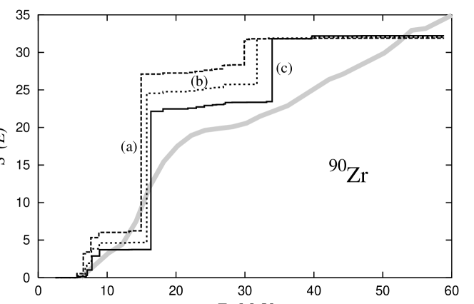
Figure 1: Distribution of $\sigma t^{-}$ strength in ${}^{90}\mathrm{Zr}$. Thick gray line is experimental distribution of the GT strength [13]. Lines labeled by (a), (b) and (c) present the results of calculations with different values of $\kappa^{01}_{1}$.

An example of such a residual interaction is given by the phenomenological separable residual interaction discussed in detail in [12],

$$H_{\mathrm{res}}=-\frac{1}{2}\sum_{L,J,M}\sum_{q\neq q^{\prime}}\left(\kappa^{LJ}_{0}+\kappa^{LJ}_{1}(\vec{\tau}_{q}\cdot\vec{\tau}_{q^{\prime}})\right)Q^{{\dagger}}_{LJM}(q)\,Q_{LJM}(q^{\prime}).$$ (15)

Here $\vec{\tau}$ are isospin Pauli matrices, and

$$Q_{LJM}(q)=i^{L}f_{LJ}(r_{q})\,[Y_{L}(\hat{r}_{q})\times\sigma_{q}]_{JM}$$

is the one-body spin-multipole operator. We have shown here the spin-multipole part of residual interaction, the expression for a multipole one can be found in [12]. The interaction with the radial form factor

$$f_{LJ}(r)=\frac{dU(r)}{dr},$$ (16)

(here $U(r)$ is central part of Saxon-Woods potential) has a surface character and may mix $\Delta N=0$ and $\Delta N\geq 2$ particle-hole excitations.

The results of calculation of the GT strength function in ${}^{90}\mathrm{Zr}$ together with the experimental data of [13], where $(93\pm 5)\%$ of the sum rule value $3(N-Z)=30$ was observed, are presented in Fig. 1. The GT strength function is shown as the running sum

$$S^{-}(E)=\int_{0}^{E}\,b^{-}(E^{\prime})\,dE^{\prime}.$$

The lines marked by (a), (b) and (c) are the theoretical strength functions calculated with $\kappa^{01}_{1}=-0.23/A$, $\kappa^{01}_{1}=-0.43/A$ and $\kappa^{01}_{1}=-0.63/A$, respectively. It is easily seen in Fig. 1 that new high-lying collective $1^{+}$ states appear. When $\left|\kappa^{01}_{1}\right|$ grows the energy of the collective state and its $B(GT)$ increase. For others spherical nuclei theoretical GT strength functions have been calculated and compared with the experimental ones in [14]. All examples confirm that for explanation of the effect of missing (quenching) of the GT strength the specific feature of nuclear residual interaction is required: there should be a strong mixing among the $\Delta N=0$ and $\Delta N\geq 2$ particle-hole configurations. The appearance of this specific feature of residual interaction should be checked in other charge-exchange processes related to spin-isospin transitions.

3 Total rates of muon capture

The spin-isospin transitions are observed in two weak interaction processes: beta-decay and muon capture. Only a small fraction of the whole GT transition strength can usually be observed in beta decay because the limited energy release and variations in the GT strength function at low excitation energy affect noticeably theoretical $ft$-values. This limitation is removed in the reaction of ordinary muon capture (OMC)

$$\mu^{-}+A(Z,N)\rightarrow\nu_{\mu}+B(Z-1,N+1),$$ (17)

where states in a wide excitation energy range can be populated due to a relatively large muon mass, $m_{\mu}\approx 105\,\mathrm{MeV}$. The phase space factor of partial OMC rate $\Lambda_{f}$ depends on the square of neutrino energy

$$E_{\nu}=\left(m_{\mu}-|\epsilon_{1S}|+M_{A}-M_{B}-E_{f}\right)\left(1-{{m_{\mu}-|\epsilon_{1S}|+M_{A}-M_{B}-E_{f}}\over{2(m_{\mu}+M_{A})}}\right),$$

where $E_{f}$ is the excitation energy in the nucleus $B$, $M_{A}$ and $M_{B}$ are the masses of initial and final nuclei, $\epsilon_{1S}$ is the muon binding energy in the muonic atom. For example, for $0^{+}\rightarrow 1^{+}$ the rate of muon capture

$$\matrix{\Lambda_{f}\sim&\displaystyle E_{\nu}^{2}\,g_{A}^{2}\biggl{\langle}1^{+}_{f}\biggl{\|}\sum_{q}j_{0}(E_{\nu}r_{q})\,\sigma_{q}\,t^{+}_{q}\biggr{\|}0^{+}_{\mathrm{g.s.}}\biggr{\rangle}^{2}\hfill\cr\vskip 3.0pt plus 1.0pt minus 1.0pt\cr{}&\displaystyle\times\biggl{\{}1+{2\over 3}\bigl{[}1+4{g_{V}+g_{M}\over g_{A}}-{g_{P}\over g_{A}}\bigr{]}{E_{\nu}\over 2M_{p}}+{1\over 3}\bigl{(}{g_{P}\over g_{A}}\,{E_{\nu}\over 2M_{p}}\bigr{)}^{2}+\ldots\biggr{\}},\hfill\cr}$$ (18)

here $M_{p}$ is the proton mass, and $g_{V}$, $g_{A}$, $g_{M}$ and $g_{P}$ are vector, axial-vector, weak-magnetic, and pseudoscalar couplings of weak nucleon current [15].

The energy released in the muon capture is comparable with muon mass; therefore, the relative error in theoretical $\Lambda_{f}$ caused by uncertainties in the theoretical strength function for the corresponding nuclear transitions is rather small

$${\Delta\Lambda_{f}\over\Lambda_{f}}\approx{\Delta E_{f}\over E_{\nu}}\ll{\Delta E_{f}\over E_{f}}$$

in comparison with the ones in beta-decay, and one can hope that calculation in the RPA, which reproduces well the general features of strength functions of the corresponding transitions, will give a reasonable description of the OMC rates. The total muon capture rate is calculated as the sum of the rates for all possible nuclear transitions

$$\Lambda_{\mathrm{tot}}=\sum_{f}\Lambda_{f}.$$

Figure 2: Total rates of OMC on complex nuclei. Open and closes circles are the calculation results; the crosses are the experimental data. See the text for details.

The total OMC rates for several even-even spherical nuclei are calculated and discussed in detail in [16]. Here we shortly present the main results. The $\Lambda_{\mathrm{tot}}$ are displayed in Fig. 2. The results of calculations, in which the separable residual interaction (15) with radial form factor (16) has been used, are shown by the closed circles. For comparison the OMC rates were calculated with the radial form factor of residual interaction

$$f_{LJ}(r)=r^{L}.$$ (19)

In Fig. 2, the corresponding $\Lambda_{\mathrm{tot}}$ are shown by the open circles. For GT transitions $L=0$, and the residual interaction with form factor (19) reduces to simple $(\vec{\sigma},\vec{\sigma})$-forces used in [17]. This interaction cannot create high-excited $1^{+}$ states and cannot reproduce the effect of missing strength, as it was shown in [17]. The experimental data extracted from [18] are pointed by the crosses and the line presents the phenomenological estimations of [19] with the parameters fitted in [18]. In the calculation the transitions from the $J^{\pi}=0^{+}$ ground state to the final states with $J^{\pi}=0^{\pm},\ldots,4^{\pm}$ were taken into account. The transitions to the states with higher momenta give negligible contributions to $\Lambda_{\mathrm{tot}}$.

Table 1: Total rates of OMC and relative contribution to $\Lambda_{\mathrm{tot}}$ of transitions to $1^{+}$ states.

Target

Theoretical results for residual interaction

with radial form factor

Figure 2 and Table 1 show that for medium-weight nuclei (from nickel to tin) the theoretical $\Lambda_{\mathrm{tot}}$, calculated with both residual interactions agree with each other and reproduce correctly the experimental rates. Table 1 shows that relative contributions to $\Lambda_{\mathrm{tot}}$ from transitions to the $1^{+}$ final states grow as the atomic number increases. For heavier nuclei (${}^{140}\mathrm{Ce}$ and ${}^{208}\mathrm{Pb}$) theoretical $\Lambda_{\mathrm{tot}}$’s overestimate the experimental data considerably. The rates calculated with the form factor (19) are smaller than those obtained with the radial part (16). Figure 3 shows that the difference comes about mainly due to capture feeding the high-excited $1^{\pm}$ states which are absent in calculations with $f_{LJ}(r)=r^{L}$.

Figure 3: OMC rates by ${}^{208}\mathrm{Pb}$. Total and partial integrated capture rates up to the excitation energy $E$ of the final nucleus. The partial rates are shown for the final states with $J^{\pi}=1^{\pm}$. Solid lines show the results of calculation with the radial form factor (16) of residual interaction, dashed lines show the same with the form factor (19). The solid vertical bars present the distribution of calculated partial rates over the excited states with $J^{\pi}=1^{\pm}$. In the upper part of the figure the distribution over all excited states is displayed.

Table 1 shows that the excitation of high-excited states diminishes the influence of neutron excess on the muon capture. In rather heavy nuclei the muon capture rates (summed over all $0^{+}\rightarrow 1^{+}$ nuclear transitions) in calculation with the form factor (16) are larger than the rates calculated with the form factor (19), and even higher than the corresponding rates obtained in the model of independent quasiparticles (without any residual interaction). The fact that in heavier nuclei theoretical $\Lambda_{\mathrm{tot}}$’s overestimate the experimental rates was found in [20], where the Landau-Migdal residual forces were used. Their theoretical $\Lambda_{\mathrm{tot}}({}^{208}\mathrm{Pb})=161\times 10^{5}\,\mathrm{s}^{-1}$ and are well compared with the value $160\times 10^{5}\,\mathrm{s}^{-1}$ obtained in calculation with the residual interaction (19).

The calculated $\Lambda_{\mathrm{tot}}$’s in heavy nuclei are found to be sensitive to the kind of residual interaction used. The largest discrepancy between the theory and experiment is obtained in the calculations with the residual interaction form factor (16). This interaction forms the high-excited final states. As it was shown above, the high-excited $1^{+}$ states are responsible for the effect of missing GT strength. So the purpose of reproducing $\Lambda_{\mathrm{tot}}$ in heavy nuclei contradicts the description of the missing GT strength.

4 Isovector $0^{+}\rightarrow 1^{+}$ transitions in $A=28$ nuclei

Unfortunately, it is impossible to extract from the experimental $\Lambda_{\mathrm{tot}}$ the capture rate determined by the $0^{+}\rightarrow 1^{+}$ nuclear transitions. One should look for partial muon capture in which the final state of a product nucleus is known. The experimental study of partial muon capture by $sd$-shell nuclei was carried out in [21]. Here we discuss the transitions observed in the reaction

$$\mu^{-}+{}^{28}\mathrm{Si}(0^{+}_{g.s})\rightarrow\nu_{\mu}+{}^{28}\mathrm{Al}(1^{+}).$$ (20)

The capture rates for transitions into three $1^{+}$ states with energies $1.620$, $2.201$ and $3.109$ MeV were measured in [21]. These three states together with the $1^{+}$ states with energies $10.90$, $11.45$ and $12.33$ MeV in ${}^{28}\mathrm{Si}$ and $1^{+}$ states with energies $1.59$, $2.10$, and $2.94$ MeV in ${}^{28}\mathrm{P}$ form three isospin triplets [22]. Starting from the $J^{\pi},T=0^{+},0$ ground state of ${}^{28}\mathrm{Si}$ the states of isospin triplets can be populated by spin-isospin probes: the states in ${}^{28}\mathrm{Al}$ — by reaction (20). Equation (18) shows that the main part of the transitional operator is proportional to $\vec{\sigma}t^{+}$. The states in ${}^{28}\mathrm{Si}$ can be excited in the reaction of electron scattering $(e,e^{\prime})$; the transitional operator is proportional to $(g_{s}\vec{\sigma}+g_{l}\vec{l}\;)t^{0}$. The corresponding experimental data are published in [23]. The states in ${}^{28}\mathrm{P}$ can be observed in $(p,n)$ reaction, in which the transition operator is proportional to $\vec{\sigma}t^{-}$; the experimental results are given in [24].

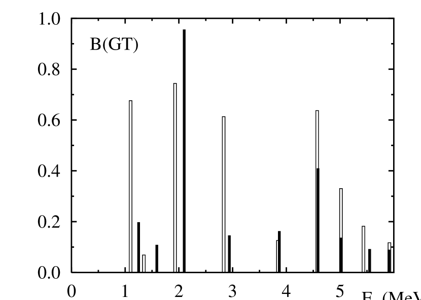
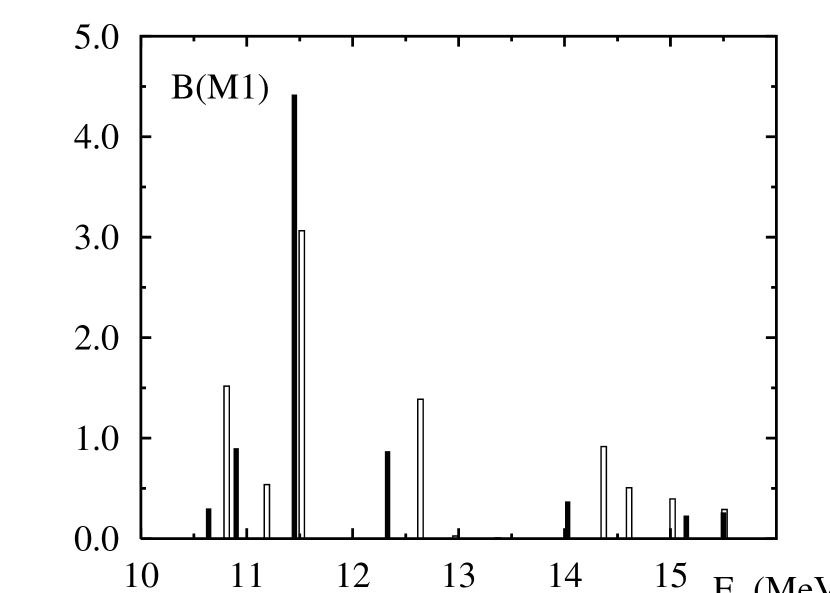
Figure 4: Isovector $0^{+}\rightarrow 1^{+}$ transitions in $A=28$ nuclei. The experimental data are presented by closed bars. Open bars are theoretical results calculated with Hamiltonian [25].

The experimental values of reduced probabilities of magnetic dipole, $B(M1)$, and GT transitions as functions of excitation energy are presented by the closed bars in Fig. 4. The open bars show the results of calculations within the multiparticle shell model with Wildenthal’s Hamiltonian [25]. The computer code OXBASH [26] was used in calculations. The $B(M1)$ values were obtained with free $g_{s}$ and $g_{l}$ factors, and no effective charges were used in $B(GT)$ calculations. In principle, one should expect introducing the effective charge because the shell model [25] works within the $sd$-shell space, and the previous discussion shows the importance of $\Delta N\geq 2$ transitions for correct description of the GT strength function, at least. In the present situation it is a difficult task to determine the effective charge because theoretical $B(M1)$ and $B(GT)$ values are higher than experimental ones for many states, except the strongest transition in which the theory goes below experiment for both $(p,n)$ and $(e,e^{\prime})$ reactions. Theoretical summed transition strengths are higher than experimental ones: $B_{\Sigma}^{\mathrm{exp}}(GT)=0.66\,B_{\Sigma}^{\mathrm{th}}(GT)$ and $B_{\Sigma}^{\mathrm{exp}}(M1)=0.85\,B_{\Sigma}^{\mathrm{th}}(M1)$. To cope with this situation, an orthogonal transformation acting in subspace of wave functions of isovector $1^{+}$ states was suggested in [27]. The parameters of the transformation were chosen such that the theoretical strength functions of GT and $M1$ transitions calculated with transformed wave functions coincided in shape (within a constant factor) with the corresponding experimental functions. Due to orthogonality of transformation, theoretical summed transition strengths are conserved, and the transformation results in redistribution of $B(GT)$’s and $B(M1)$’s over excitation energy. The transformed strength functions are presented in Fig. 5.

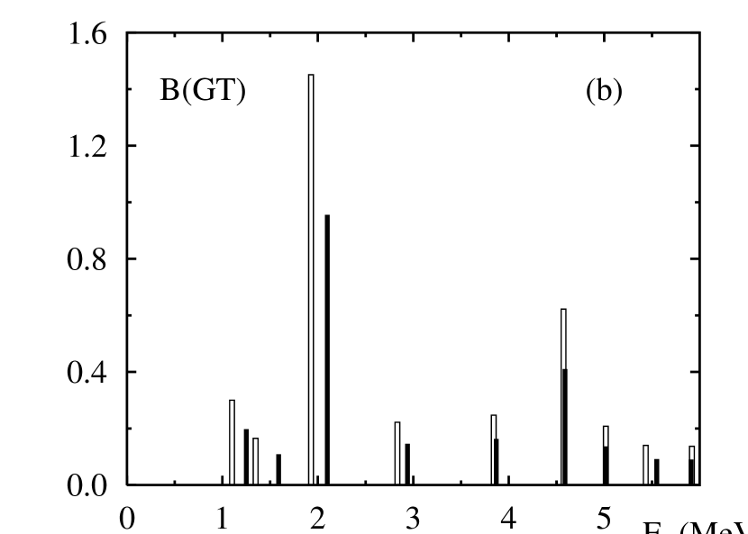
Figure 5: Properties of isovector transitions in $A=28$ nuclei calculated with transformed wave functions.

The transformation established exact proportionality between theoretical and experimental GT strength functions and approximate proportionality for $M1$ strength functions.

Table 2: Properties of isovector $1^{+}$ states in $A=28$ nuclei; $\tau$– life-time; $\gamma$– $\gamma$-decay branching ratios; $\Lambda_{f}$ – partial OMC rate.

Nucleus	Observable	Experiment		Theory
		Value	Ref.	(a)	(b)
${}^{28}\mathrm{Al}$	$\tau(1^{+}_{2.201})$ (in fs)	$59\pm 6$ $51\pm 1.0_{\mathrm{stat.}}\pm 6.7_{\mathrm{sys.}}$	[28] [29]	66	49
	$\gamma(1^{+}_{2.201}\to 2^{+}_{0.031})$ (in %)	$79$	[22]	$2$	$63$
	$\gamma(1^{+}_{2.201}\to 0^{+}_{0.972})$ (in %)	$16$		$80$	$35$
${}^{28}\mathrm{Al}$	$\Lambda(1^{+}_{1.620})$ (in $10^{3}\,\mathrm{s}^{-1}$)	$12.9\pm 2.1$	[21]	$3.1$	$7.6$
	$\Lambda(1^{+}_{2.201})$ (in $10^{3}\,\mathrm{s}^{-1}$)	$62.8\pm 7.4$		$34.1$	$63.6$
	$\Lambda(1^{+}_{3.110})$ (in $10^{3}\,\mathrm{s}^{-1}$)	$14.7\pm 2.6$		$26.1$	$11.2$
${}^{28}\mathrm{Si}$	$B_{M1}(1^{+}_{10.90})$ ($\mu_{N}$)	$0.90\pm 0.02$	[23]	$0.54$	$1.04$
	$B_{M1}(1^{+}_{11.45})$ ($\mu_{N}$)	$4.42\pm 0.20$		$3.06$	$4.46$
	$B_{M1}(1^{+}_{12.33})$ ($\mu_{N}$)	$0.87\pm 0.06$		$1.39$	$0.76$
${}^{28}\mathrm{P}$	$B_{GT}^{-}(1^{+}_{1.59})$	$0.109\pm 0.002$	[24]	$0.069$	$0.165$
	$B_{GT}^{-}(1^{+}_{2.10})$	$0.956\pm 0.005$		$0.774$	$1.451$
	$B_{GT}^{-}(1^{+}_{2.94})$	$0.146\pm 0.003$		$0.613$	$0.222$

The characteristics of partial transitions to the members of isospin triplets are collected in Table 2. Theoretical values calculated with the initial wave functions (column (a)) and with transformed wave functions (column (b)) are presented in Table 2 for comparison. The muon capture rates were calculated with free values of weak nucleon current couplings. The transformation of the wave functions of excited states improves greatly the description of muon capture rates, and for the strongest transition the theoretical rate coincides with experiment. The calculation with the transformed wave functions reproduces correctly the experimental $B(M1)$ values. However, there is a considerable disagreement between theoretical (b) and experimental $B(GT)$’s. It is an unexpected result because the spin-isospin parts of the operators describing the charge-exchange reactions, magnetic scattering of electrons, and muon capture are practically the same. The discrepancy between theoretical and experimental $B(GT)$ values indicates that the relation between the cross sections of charge-exchange reactions and $B(GT)$’s may be complicated even for strong transitions.

5 Conclusion

The energy weighted moments of strength function of GT transition, $S^{\pm}_{k}$, are calculated in the RPA, SRPA and within the fragmentation problem. Considering $S^{-}_{0}$ and $S^{-}_{1}$ we have shown that the effect of missing GT strength should be reproduced as the result of interaction among the particle-hole excitations, without including the 2p–2h configurations. Hence, the residual interaction in the spin-isospin channel must intensively mix the $\Delta N=0$ and $\Delta N\geq 2$ particle-hole states. The example of this interaction is presented. It is shown that the experimental strength function of $\sigma t^{-}$ transition in ${}^{90}\mathrm{Zr}$ can be reproduced rather well in the whole region of excitation energy.

Total muon capture rates were calculated for several nuclei using two variants of residual interaction. Theoretical total rates of muon capture by medium nuclei practically do not depend on the residual interaction used in calculation. In heavy nuclei theoretical rates are higher than experimental ones. The excess depends on the residual interaction, and the difference between theory and experiment is the largest when the residual interaction, which forms the high-excited collective states, is used in the calculation. The existence of these states is assumed by the effect of missing GT strength.

It is shown that the distributions of transition strength over the excitation energy in $A=28$ nuclei extracted from weak and electromagnetic processes are in conflict with the ones obtained from charge-exchange nuclear reactions. In particular, no quenching of spin-isospin transitions is found in the rates of partial allowed muon capture ${}^{28}\mathrm{Si}(0^{+}_{g.s})(\mu,\nu){}^{28}\mathrm{Al}(1^{+})$.

References

- [1] D. J. Rowe, Rev. Mod. Phys., 40, 153, (1968)
- [2] A. M. Lane and J. Martorell, Ann. Phys., 129, 273, (1980)
- [3] F. Gantmacher, Theory of Matrices, vol. 2, AMS Publishing, 2000
- [4] S. Drożdż, S. Nishizaki, J. Speth and J. Wambach, Phys. Rep., 197, 1, (1990)
- [5] A. Bohr and B. R. Mottelson, Nuclear Structure, vol. 1, New York, Amsterdam, 1969
- [6] V. V. Voronov and V. G. Soloviev, Fiz. Elem. Chast. At. Yadra, 14, 1380, (1983) [Sov. J. Part. Nucl., 14, 583 (1983)]
- [7] V. A. Kuz’min, Theoret. i Matemat. Fiz., 70, 315 (1987) [Theor. and Math. Phys., 70, 223 (1987)]
- [8] G. F. Bertsch, P. F. Bortignon and R. A. Broglia, Rev. Mod. Phys., 55, 287 (1983)
- [9] G. J. Mathews, S. D. Bloom and R. F. Hausman, Jr., Phys. Rev. C, 28, 1367 (1983)
- [10] S. Drożdż, V. Klempt, J. Speth, and J. Wambach, Phys. Lett. B, 166, 18 (1986)
- [11] S. Drożdż, F. Osterfeld, J. Speth, J. Wambach, Phys. Lett. B, 189, 271 (1987)
- [12] A. I. Vdovin and V. G. Soloviev, Fiz. Elem. Chast. At. Yadra, 14, 237, (1983) [Sov. J. Part. Nucl., 14, 99 (1983)]
- [13] T. Wakasa et al., Phys. Rev. C, 56, 2909, (1997)
- [14] V. A. Kuz’min, Yad. Fiz., 58, 418, (1995) [Phys. Atom. Nucl.. 58, 368, (1995)]; K. Junker, V. A. Kuz’min, T. V. Tetereva, Eur. Phys. J. A, 5, 37 (1999)
- [15] V. V. Balashov, G. Ya. Korenman, R. A. Eramzhyan, Poglozhenie mezonov atomnymi yadrami, M., Atomizdat, 1978, 294 pp (in Russian)
- [16] R. A. Eramzhyan, V. A. Kuz’min, and T. V. Tetereva, Nucl. Phys. A, 642, 428 (1998); V. A. Kuzmin, T. V. Tetereva, K. Junker, and A. A. Ovchinnikova, J. Phys. G: Nucl. Part. Phys., 28, 665 (2002)
- [17] C. Gaarde et al., Nucl. Phys. A, 369, 258 (1981)
- [18] T. Suzuki, D. F. Measday, and J. P. Roalsvig, Phys. Rev. C, 35, 2212 (1987)
- [19] B. Goulard and H. Primakoff, Phys. Rev. C, 10, 2034 (1974)
- [20] E. Kolbe, K. Langanke, and P. Vogel, Phys. Rev. C, 62, 055502 (2000)
- [21] T. P. Gorringe, et al., Phys. Rev. C, 60, 055501 (1999)
- [22] P. M. Endt, Nucl. Phys. A, 521, 1 (1990)
- [23] C. Lüttge, et al., Phys. Rev. C, 53, 127 (1996); Y. Fujita, et al., Phys. Rev. C, 55, 1137 (1996)
- [24] P. von Neumann-Cosel, A. Richter, Y. Fujita and B. D. Anderson, Phys. Rev. C, 55, 532 (1997)
- [25] B. H. Wildenthal, Prog. Part. Nucl. Phys., 11, 5 (1984)
- [26] A. Etchegoyen., B. A. Brown, W. D. M. Rae, MSUCL Report No. 524, Michigan, 1986
- [27] V. A. Kuz’min and T. V. Tetereva, Yad. Fiz., 63, 1966 (2000) [Phys. At. Nucl., 63, 1874 (2000)]
- [28] P. M. Endt, Nucl. Phys. A, 633, 1 (1998)
- [29] Ch. Briançon, et al., Nucl. Phys. A, 671, 647 (2000)