Recent progress on understanding “pasta” phases in dense stars

Abstract

In cores of supernovae and crusts of neutron stars, nuclei can adopt interesting shapes, such as rods or slabs, etc., which are referred to as nuclear “pasta.” Recently, we have been studying the pasta phases focusing on their dynamical aspects with quantum molecular dynamic (QMD) approach. We review our findings on the following topics: dynamical formation of the pasta phases by cooling down the hot uniform nuclear matter; a phase diagram on the density versus temperature plane; structural transitions between the pasta phases induced by compression and their mechanism. Properties of the nuclear interaction used in our works are also discussed.

1 I. Introduction

In ordinary matter, atomic nuclei are roughly spherical. This may be understood in the liquid drop picture of the nucleus as being a result of the forces due to the surface tension of nuclear matter, which favors a spherical nucleus, being greater than those due to the electrical repulsion between protons, which tends to make the nucleus deform. When the density of matter approaches that of atomic nuclei, i.e., the normal nuclear density $\rho_{0}$, nuclei are closely packed and the effect of the electrostatic energy becomes comparable to that of the surface energy. Consequently, at subnuclear densities around $\rho\simeq\rho_{0}/2$, the energetically favorable configuration is expected to have remarkable structures: the nuclear matter region (i.e., the liquid phase) is divided into periodically arranged parts of rodlike or slablike shape, embedded in the gas phase and in a roughly uniform electron gas. Besides, there can be phases in which nuclei are turned inside out, with cylindrical or spherical bubbles of the gas phase in the liquid phase. These phases with nonspherical nuclei are often referred to as nuclear “pasta” phases because nuclear slabs and rods look like “lasagna” and “spaghetti.” Likewise, spherical nuclei and bubbles are called “meatballs” and “cheese,” respectively.

In equilibrium dense matter in supernova cores and neutron stars, existence of the pasta phases has been predicted by Ravenhall et al. rpw and Hashimoto et al. hashimoto . Since these seminal works, properties of the pasta phases in equilibrium states have been investigated with various nuclear models. They include studies on phase diagrams at zero temperature lorenz ; oyamatsu ; sumiyoshi ; gentaro ; williams and at finite temperatures lassaut . These earlier works have confirmed that, for various nuclear models, the nuclear shape changes as: $\mbox{sphere}\rightarrow\mbox{cylinder}\rightarrow\mbox{slab}\rightarrow\mbox{cylindrical hole}\rightarrow\mbox{spherical hole}\rightarrow\mbox{uniform}$, with increasing density.

In these earlier works, however, a liquid drop model or the Thomas-Fermi approximation is used with an assumption on the nuclear shape (except for Ref. williams ). Thus the phase diagram at subnuclear densities and the existence of the pasta phases should be examined without assuming the nuclear shape. It is also noted that at temperatures of several MeV, which are relevant to the collapsing cores, effects of thermal fluctuations on the nucleon distribution are significant. However, these thermal fluctuations cannot be described properly by mean-field theories such as the Thomas-Fermi approximation used in the previous work lassaut .

In contrast to the equilibrium properties, dynamical or non-equilibrium aspects of the pasta phases had not been studied until recently except for some limited cases formation ; review . Thus it had been unclear even whether or not the pasta phases can be formed and the transitions between them can be realized during the collapse of stars and the cooling of neutron stars, which have finite time scales.

To solve the above problems, molecular dynamic approaches for nucleon many-body systems are suitable. They treat the motion of the nucleonic degrees of freedom and can describe thermal fluctuations and many-body correlations beyond the mean-field level.

Using the framework of QMD aichelin , which is one of the molecular dynamic methods, we have solved the following two major questions qmd_transition ; qmd_cold ; qmd_hot .

• Question 1: Whether or not the pasta phases are formed by cooling down hot uniform nuclear matter in a finite time scale much smaller than that of the neutron star cooling?

• Question 2: Whether or not transitions between the pasta phases can occur by the compression during the collapse of a star?

The pasta phases have recently begun to attract the attention of many researchers (see, e.g., Refs. burrows ; martinez and references therein). The mechanism of the collapse-driven supernova explosion has been a central mystery in astrophysics for almost half a century (e.g., Ref. bethe ). Previous studies suggest that the revival of the shock wave by neutrino heating is a crucial process. As has been pointed out in Refs. gentaro ; qmd_cold and elaborated in Refs. horowitz1 ; horowitz2 ; future , the existence of the pasta phases instead of uniform nuclear matter increases the neutrino opacity of matter in the inner core significantly due to the neutrino coherent scattering by nuclei freedman ; sato ; this affects the total energy transferred to the shocked matter. Thus the pasta phases could play an important role in the future study of supernova explosions. Our recent work qmd_transition strongly suggests the possibility of dynamical formation of the pasta phases from a crystalline lattice of spherical nuclei; effects of the pasta phases on the supernova explosions should be seriously discussed in the near future.

2 II. Method: Quantum Molecular Dynamics

Among various versions of the molecular dynamic models, Quantum Molecular Dynamics (QMD) aichelin is the most practical one for investigating the pasta phases. Rodlike and slablike nuclei are mesoscopic entities of nuclei themselves and they contain a large number of nucleons. QMD, which is a less elaborate in the treatment of the exchange effect, allows us to study such large systems with several nonspherical nuclei. The typical length scale $r_{\rm c}$ of half of the inter-structure is $r_{\rm c}\sim 10$ fm and the density region of interest is around half of the normal nuclear density $\rho_{0}$. The total nucleon number $N$ necessary to reproduce $n$ structures in the simulation box is $N\sim\rho_{0}(2r_{\rm c}n)^{3}$ (for slabs). It is thus desirable to use $\sim 10^{4}$ nucleons in order to reduce boundary effects. Such large systems are difficult to be handled by other molecular dynamic models such as FMD fmd and AMD amd , whose calculation costs increase as $\sim N^{4}$, but are tractable for QMD, whose calculation costs increase as $\sim N^{2}$.

It is also noted that the exchange effect is less important for the nuclear pasta structures, which are in the macroscopic scale for nucleons. This can be seen by comparing the typical values of the exchange energy and of the energy difference between pasta phases. Suppose there are two identical nucleons, $i=1$ and 2, bound in different nuclei. The exchange energy between these particles is calculated as an exchange integral: $I=\int U({\bf r}_{1}-{\bf r}_{2})\ \varphi_{1}({\bf r}_{1})\varphi_{1}^{*}({\bf r}_{2})\varphi_{2}({\bf r}_{2})\varphi_{2}^{*}({\bf r}_{1})\ d{\bf r}_{1}d{\bf r}_{2}\$, where $U$ is the potential energy. An asymptotic form of the wave function is given by $\varphi_{i}\sim\exp{(-k_{i}r)}$ with $k_{i}=\sqrt{2mE_{i}}/\hbar\ ,\ (i=1,2)$, where $E_{i}$ is the binding energy and $m$ is the nucleon mass. The exchange integral reads $I\sim\exp{[-(k_{1}+k_{2})R]}\sim 5\times 10^{-6}$ MeV for the internuclear distance $R\simeq 10$ fm and $E_{i}\simeq 8$ MeV, which is extremely smaller than the typical energy difference per nucleon between different pasta phases of order 0.1 keV (for neutron star matter) - 10 keV (for supernova matter). Therefore, it is expected that QMD is not a bad approximation for investigating the pasta phases.

2.1 1. Model Hamiltonian and its Properties

In our studies on the pasta phases, we have used a nuclear force given by a QMD model Hamiltonian with the medium-equation-of-state parameter set in Ref. maruyama . This model Hamiltonian consists of six parts:

$${\cal H}=K+V_{\rm Pauli}+V_{\rm Skyrme}+V_{\rm sym}+V_{\rm MD}+V_{\rm Coulomb}\ ,$$ (1)

where $K$ is the kinetic energy; $V_{\rm Pauli}$ is the momentum-dependent “Pauli potential,” which reproduces the effects of the Pauli principle phenomenologically; $V_{\rm Skyrme}$ is the Skyrme potential which consists of an attractive two-body term and a repulsive three-body term; $V_{\rm sym}$ is the symmetry potential; $V_{\rm MD}$ is the momentum-dependent potential introduced as two Fock terms of the Yukawa interaction; $V_{\rm Coulomb}$ is the Coulomb energy between protons.

The parameters in the Pauli potential are determined to fit the kinetic energy of the free Fermi gas at zero temperature. The above model Hamiltonian reproduces the binding energy of symmetric nuclear matter, 16 MeV per nucleon, at the normal nuclear density $\rho_{0}=0.165$ fm^-3 and other saturation properties: the incompressibility is set to be 280 MeV and the symmetry energy is 34.6 MeV. This model Hamiltonian also well reproduce the properties of stable nuclei relevant to our interest: the binding energy except for light nuclei from ¹²C to ²⁰Ne maruyama , and the rms radius of the ground state of heavy ones with $A\gtrsim 100$ kido . It is also confirmed that another QMD Hamiltonian close to this model provides a good description of nuclear reactions including the low energy region (several MeV per nucleon) niita .

Let us then examine other properties of the nuclear interaction (at zero temperature), which have not been determined accurately yet but have important effects on inhomogeneous structure of matter at subnuclear densities. Such quantities are the nuclear surface tension $E_{\rm surf}$, the energy per nucleon $\epsilon_{\rm n}$ of the pure neutron matter, and the proton chemical potential $\mu_{\rm p}^{(0)}$ in the pure neutron matter. The surface tension $E_{\rm surf}$, which is the most important among these three quantities, controls the size of the nuclei and bubbles, and hence the sum of the Coulomb and surface energies. With increasing $E_{\rm surf}$ and so this energy sum, the density $\rho_{\rm m}$ at which matter becomes uniform is lowered. There is a tendency, especially in a case of neutron star matter, that the higher $\epsilon_{\rm n}$, $\rho_{\rm m}$ is lowered. This is because larger $\epsilon_{\rm n}$ tends to favor uniform nuclear matter without dripped neutron gas regions than mixed phases. In neutron star matter, there is also a tendency that the lower $\mu_{\rm p}^{(0)}$, the smaller $\rho_{\rm m}$. This is because $-\mu_{\rm p}^{(0)}$ represents the degree to which the neutron gas outside the nuclei favors the presence of protons in itself.

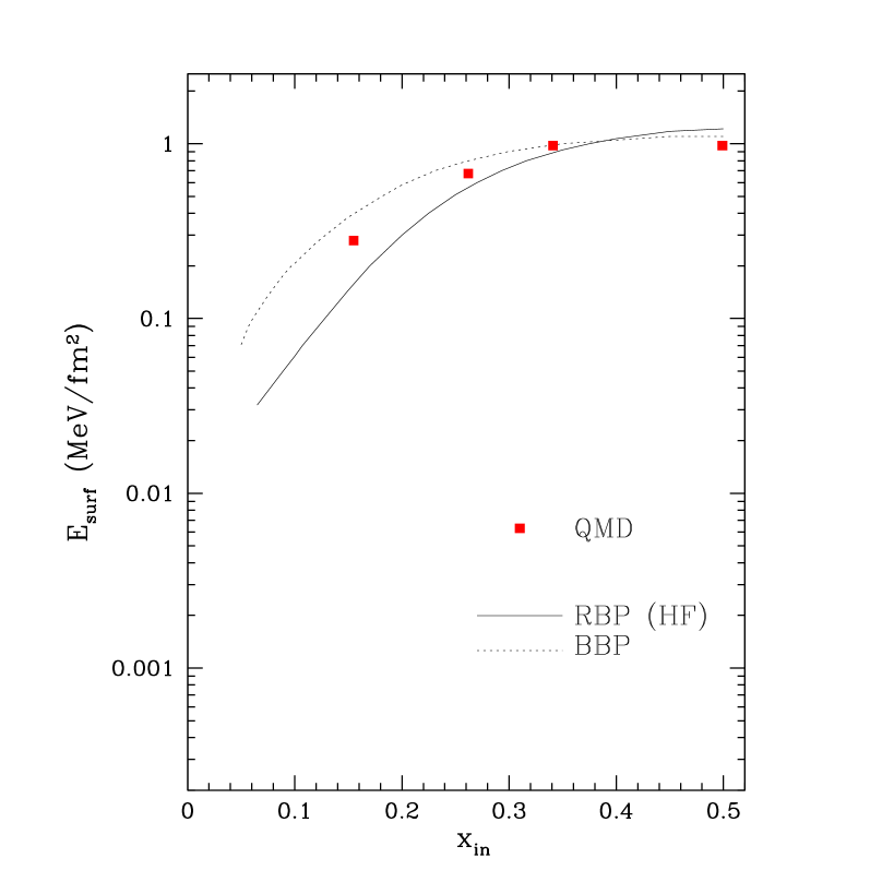
Figure 1: (Color) The nuclear surface energy per unit area (the surface tension) $E_{\rm surf}$ versus the proton fraction $x_{\rm in}$ in the nuclear matter region. The red solid squares are the values of the present QMD Hamiltonian maruyama ; the solid curve is the result of the Skyrme-Hartree-Fock calculation with a modified version of 1’ parameter set done by Ravenhall, Bennett and Pethick (RBP) rbp ; the dotted curve is from Baym, Bethe and Pethick (BBP) bbp . This figure is adapted from Ref. qmd_cold .

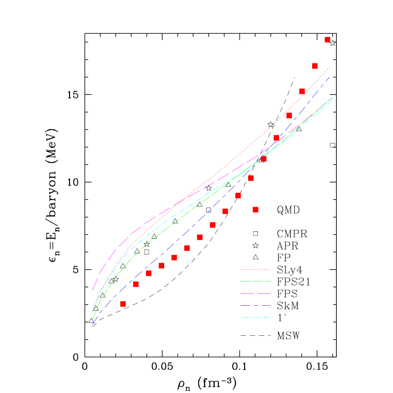
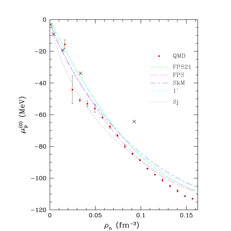
Figure 2: (Color) The neutron density $\rho_{\rm n}$ dependence of the energy per nucleon $\epsilon_{\rm n}$ (left panel) and the proton chemical potential $\mu_{\rm p}^{(0)}$ (right panel) of pure neutron matter. The red solid squares show the result of the present QMD model Hamiltonian maruyama . The red dotted line denoted by SLy4 is the result from Ref. douchin , and the colored broken lines as marked by the other Skyrme interactions (FPS21, 1’, FPS and SkM) are the results summarized by Pethick, Ravenhall and Lorenz prl . The black dotted line is the result of Sjöberg sj and the black dashed line is that of Myers, Swiatecki and Wang msw . The open squares shows the result of the GFMC calculation by Carlson et al. gfmc ; the open stars denote the values obtained by Akmal, Pandharipande and Ravenhall akmal ; the triangles are those from Friedman and Pandharipande fp ; the crosses from Siemens and Pandharipande siemens . The large error bars and the scatter of $\mu_{\rm p}^{(0)}$ of QMD in the low density region $\rho\lesssim 0.3\rho_{0}$ are due to the local roughness of the density in the neutron matter, which is caused by the fixed width of the wave packet. This figure is adapted from Ref. qmd_cold .

In Figs. 1 and 2, we have plotted the results of these quantities for the present model Hamiltonian. We can say that, on the whole, they give reasonable values within uncertainties of each quantities. It is noted that $E_{\rm surf}$ of the present model shows moderate values between the RBP and BBP results. The behavior of $\mu_{\rm p}^{(0)}$ is also in a reasonable agreement with various Skyrme-Hartree-Fock calculations except for higher densities of $\rho_{\rm n}\gtrsim 0.1$ fm^-3 relevant only for neutron star matter just below $\rho_{\rm m}$. The quantity $\epsilon_{\rm n}$, however, shows some deviation from the major trend of Skyrme-Hartree-Fock results and of the values of the microscopic calculations. The behavior of $\epsilon_{\rm n}$ of the present model is similar to that of the SkM interaction and of the interaction by Myers et al. msw .

In the following, for each case of different value of the proton fraction $x$ of matter, we summarize the consequences of the features of $E_{\rm surf}$, $\epsilon_{n}$ and $\mu_{p}^{(0)}$ of the present QMD interaction.

• For symmetric nuclear matter ($x=x_{\rm in}=0.5$)

  According to $E_{\rm surf}$ at $x_{\rm in}=0.5$, the present model is consistent with the other results, and is an appropriate effective interaction for studying the pasta phases at $x=0.5$.

• For neutron star matter ($x\lesssim 0.1$)

  The melting density $\rho_{\rm m}$ is lowered by larger $E_{\rm surf}$, steep rise of $\epsilon_{\rm n}$ at $\rho\gtrsim 0.12$ fm^-3 and larger negative values of $\mu_{\rm p}^{(0)}$ at $\rho\gtrsim 0.1$ fm^-3 compared to various Skyrme-Hartree-Fock calculations.

• For supernova matter ($x\sim 0.3$)

  Relatively low $\epsilon_{\rm n}$ at low neutron densities $\lesssim 0.1$ fm^-3 acts to favor mixed phases rather than the uniform phase and $E_{\rm surf}$ acts in the opposite way in comparison with the Skyrme-Hartree-Fock result by RBP rbp .

3 III. Simulations and Results

Using the framework of QMD, we have solved the two major questions posed in the beginning of this article qmd_transition ; qmd_cold ; qmd_hot . In the present section, we will review these works . Hereafter, we set the Boltzmann constant $k_{\rm B}=1$.

In our simulations, we treated the system which consists of neutrons, protons, and electrons in a cubic box with periodic boundary condition. The system is not magnetically polarized, i.e., it contains equal numbers of protons (and neutrons) with spin up and spin down. The relativistic degenerate electrons which ensure charge neutrality are regarded as a uniform background review (see Refs. screening ; screen_maruyama for effects of the electron screening). The Coulomb interaction is calculated by the Ewald method taking account of the Gaussian charge distribution of the proton wave packets.

3.1 1. Realization of the Pasta Phases and Equilibrium Phase Diagrams

In Refs. qmd_cold ; qmd_hot , we have reproduced the pasta phases from hot uniform nuclear matter and discussed phase diagrams at zero and finite temperatures. In these works, we first prepared a uniform hot nucleon gas at the temperature $T\sim 20$ MeV as an initial condition, which is equilibrated for $\sim 500-2000$ fm/$c$ in advance. To realize the ground state of matter, we then cooled it down slowly until the temperature got $\sim 0.1$ MeV or less for $O(10^{3}-10^{4})$ fm/$c$, keeping the nucleon number density constant. In the cooling process, we mainly used the frictional relaxation method (equivalent to the steepest descent method), which is given by the QMD equations of motion plus small friction terms. In the case of finite temperatures, we also used thermostat to reproduce the equilibrium states.

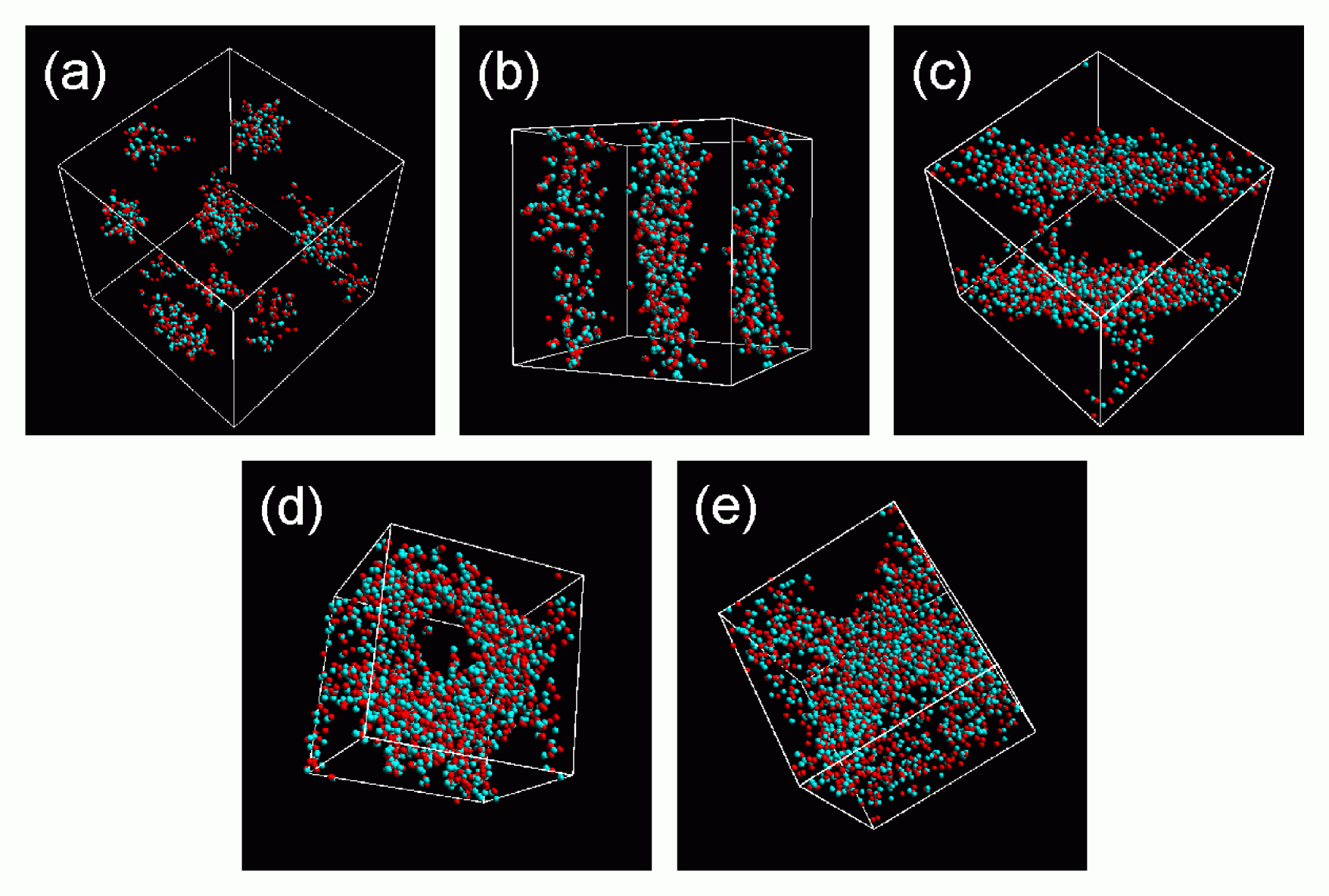
Figure 3: (Color) Nucleon distributions of the pasta phases in cold matter at $x=0.5$; (a) sphere phase, $0.1\rho_{0}$ ($L_{\rm box}=43.65\ {\rm fm}$, $N=1372$); (b) cylinder phase, $0.225\rho_{0}$ ($L_{\rm box}=38.07\ {\rm fm}$, $N=2048$); (c) slab phase, $0.4\rho_{0}$ ($L_{\rm box}=31.42\ {\rm fm}$, $N=2048$); (d) cylindrical hole phase, $0.5\rho_{0}$ ($L_{\rm box}=29.17\ {\rm fm}$, $N=2048$) and (e) spherical hole phase, $0.6\rho_{0}$ ($L_{\rm box}=27.45\ {\rm fm}$, $N=2048$), where $L_{\rm box}$ is the box size and $N$ is the total number of nucleons. The whole simulation box is shown in this figure. The red particles represent protons and the green ones neutrons. Taken from Ref. qmd_hot .

The resultant typical nucleon distributions of cold matter at subnuclear densities are shown in Fig. 3 for proton fraction of matter $x=0.5$. We can see from these figures that the phases with rodlike and slablike nuclei, cylindrical and spherical bubbles, in addition to the phase with spherical nuclei are reproduced. The above simulations have shown that the pasta phases can be formed dynamically from hot uniform matter within a time scale of $\sim O(10^{3}-10^{4})$ fm/$c$.

We show snapshots of nucleon distributions at $T=1,2$ and 3 MeV for a density $\rho=0.225\rho_{0}$ in Fig. 4. This density corresponds to the phase with rodlike nuclei at $T=0$. From these figures, we can see the following qualitative features: at $T\simeq 1.5-2$ MeV (but snapshots for $T\simeq 1.5$ MeV are not shown), the number of the evaporated nucleons becomes significant; at $T\gtrsim 3$ MeV, nuclei almost melt and the spatial distribution of the nucleons are rather smoothed out.

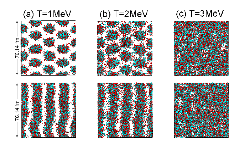
Figure 4: (Color) Nucleon distributions for $x=0.5$, $\rho=0.225\rho_{0}$ at the temperatures of 1, 2 and 3MeV. The total number of nucleons $N=16384$ and the box size $L_{\rm box}=76.14$ fm. The upper panels show the top views along the axis of the cylindrical nuclei at $T=0$, the lower ones the side views. Protons are represented by the red particles, and neutrons by the green ones. Taken from Ref. qmd_hot .

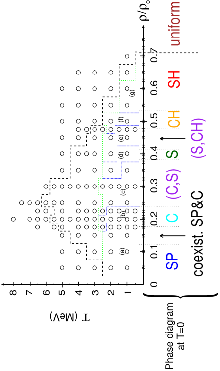
Figure 5: (Color) Phase diagram of matter at $x=0.5$ plotted in the $\rho$ - $T$ plane. The dashed and the dotted lines on the diagram show the phase separation line and the limit below which the nuclear surface can be identified, respectively. The dash-dotted lines are the phase boundaries between the different nuclear shapes. The symbols SP, C, S, CH, SH, U stand for nuclear shapes, i.e., sphere, cylinder, slab, cylindrical hole, spherical hole and uniform, respectively. The parentheses (A,B) show intermediate phases between A and B-phases with negative $\chi$, which are different from coexistence phases of them. The regions (a)-(g) correspond to the nuclear shapes characterized by $\int_{\partial R}HdA$ and $\chi$ as follows: (a) $\int_{\partial R}HdA>0,\ \chi>0$; (b) $\int_{\partial R}HdA>0,\ \chi=0$; (c) $\int_{\partial R}HdA>0,\ \chi<0$; (d) $\int_{\partial R}HdA=0,\ \chi=0$; (e) $\int_{\partial R}HdA<0,\ \chi<0$; (f) $\int_{\partial R}HdA<0,\ \chi=0$; (g) $\int_{\partial R}HdA<0,\ \chi>0$. Simulations have been carried out at points denoted by circles. Adapted from Ref. qmd_cold

When we try to classify the nuclear structure systematically, the integral mean curvature and the Euler characteristic (see, e.g., Ref. minkowski and references therein) are useful. Suppose there is a set of regions $R$, where the density is higher than a threshold density $\rho_{\rm th}$. The integral mean curvature and the Euler characteristic for the surface of this region $\partial R$ are defined as surface integrals of the mean curvature $H=(\kappa_{1}+\kappa_{2})/2$ and the Gaussian curvature $G=\kappa_{1}\kappa_{2}$, respectively; i.e., $\int_{\partial R}HdA$ and $\chi\equiv\frac{1}{2\pi}\int_{\partial R}GdA$, where $\kappa_{1}$ and $\kappa_{2}$ are the principal curvatures and $dA$ is the area element of the surface of $R$. The Euler characteristic $\chi$ depends only on the topology of $R$ and is expressed as $\chi=$ (number of isolated regions) $-$ (number of tunnels) $+$ (number of cavities). Using a combination of these two quantities calculated for nuclear surface , each pasta phase can be represented uniquely, i.e., for the phase with spherical nuclei: $\int_{\partial R}HdA>0,\ \chi>0$, cylindrical nuclei: $\int_{\partial R}HdA>0,\ \chi=0$, slablike nuclei: $\int_{\partial R}HdA=0,\ \chi=0$, cylindrical bubbles: $\int_{\partial R}HdA<0,\ \chi=0$, and spherical bubbles: $\int_{\partial R}HdA<0,\ \chi>0$. We note that the value of $\chi$ for the ideal pasta phases is zero except for the phase with spherical nuclei or spherical bubbles with positive $\chi$; negative $\chi$ is not obtained for the pasta phases.

The phase diagram obtained for $x=0.5$ is plotted in Fig. 5. As shown above, nuclear surface can be identified typically at $T\lesssim 3$ MeV (see the dotted lines) in the density range of interest. Thus the regions between the dotted line and the dashed line correspond to some non-uniform phase, which is however difficult to be classified into specific phases because the nuclear surface cannot be identified well.

In the region below the dotted lines, where we can identify the nuclear surface, we have obtained the pasta phases with spherical nuclei [region (a)], rodlike nuclei [region (b)], slablike nuclei [region (d)], cylindrical holes [region (f)] and spherical holes [region (g)]. It is noted that in addition to these pasta phases, structures with negative $\chi$ have been also obtained in the regions of (c) and (e); matter consists of multiply connected nuclear and bubble regions (i.e., spongelike structure) with branching rodlike nuclei, perforated slabs and branching bubbles, etc. A detailed discussion on the phase diagrams is given in Ref. qmd_hot .

3.2 2. Structural Transitions between the Pasta Phases

In Ref. qmd_transition , we have approached the second question asked at the beginning of this article. We have performed QMD simulations of the compression of dense matter and have succeeded in simulating the transitions between rodlike and slablike nuclei and between slablike nuclei and cylindrical bubbles.

The initial conditions of the simulations are samples of the columnar phase ($\rho=0.225\rho_{0}$) and of the laminar phase ($\rho=0.4\rho_{0}$) of 16384-nucleon system at $x=0.5$ and $T\simeq 1$ MeV. These are obtained in Ref. qmd_hot , which are presented in the last section. We then adiabatically compressed the above samples by increasing the density at the average rate of $\simeq$1.3$\times 10^{-5}\rho_{0}/$(fm$/c$) for the initial condition of the columnar phase and $\simeq$7.1$\times 10^{-6}\rho_{0}/$(fm$/c$) for that of the laminar one. According to the typical value of the density difference between each pasta phase, $\sim 0.1\rho_{0}$ (see Fig. 5), we increased the density to the value corresponding to the next pasta phase taking the order of $10^{4}$ fm$/c$, which was much longer than the typical time scale of the nuclear fission, $\sim 1000$ fm$/c$. Thus the above rates ensured the adiabaticity of the simulated compression process with respect to the change of nuclear structure. Finally, we relaxed the compressed sample at $\rho=0.405\rho_{0}$ for the former case and at $0.490\rho_{0}$ for the latter one. These final densities are those of the phase with slablike nuclei and cylindrical bubbles, respectively, in the equilibrium phase diagram at $T\simeq 1$ MeV (see Fig. 5).

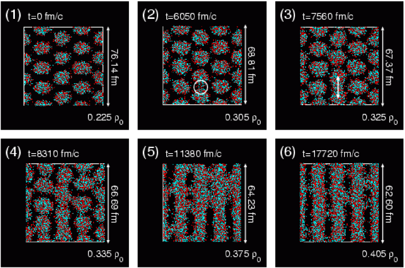
Figure 6: (Color) Snapshots of the transition process from the phase with rodlike nuclei to the phase with slablike nuclei (the whole simulation box is shown). The red particles show protons and the green ones neutrons. After neighboring nuclei touch as shown by the circle in Fig. 6-(2), the “compound nucleus” elongates along the arrow in Fig. 6-(3). The box size is rescaled to be equal in this figure. Adapted from Ref. qmd_transition .

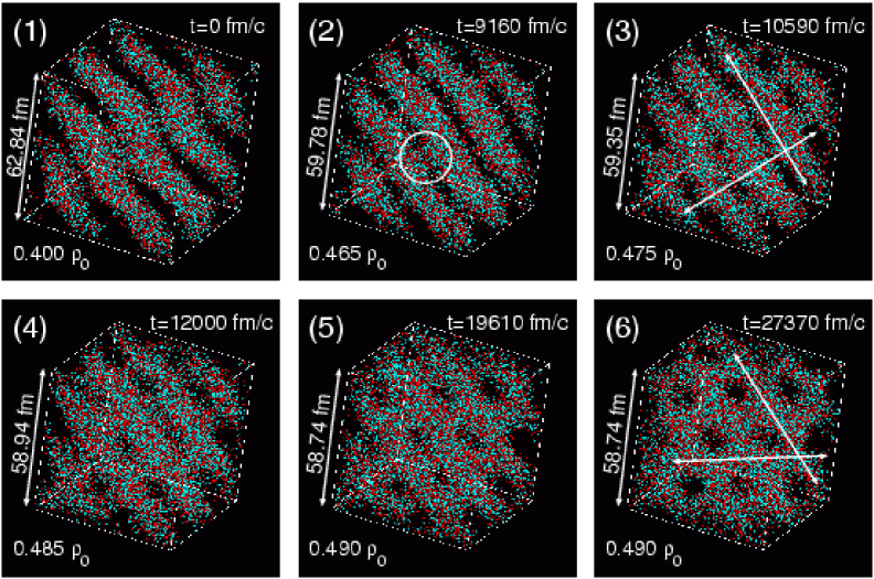
Figure 7: (Color) The same as Fig. 1 for the transition from the phase with slablike nuclei to the phase with cylindrical holes (the box size is not rescaled in this figure). After the slablike nuclei begin to touch [see the circle in Fig. 7-(2)], the bridges first crosses them almost orthogonally as shown by the arrows in Fig. 7-(3). Then the cylindrical holes are formed and they relax into a triangular lattice, as shown by the arrows in Fig. 7-(6). Adapted from Ref. qmd_transition .

The resulting time evolution of the nucleon distribution is shown in Figs. 6 and 7. As can be seen from Fig. 6, the phase with slablike nuclei is finally formed [Fig. 6-(6)] from the phase with rodlike nuclei [Fig. 6-(1)]. The temperature in the final state is $\simeq 1.35$ MeV. It is noted that the transition is triggered by thermal fluctuation, not by the fission instability: when the internuclear spacing becomes small enough and once some pair of neighboring rodlike nuclei touch due to thermal fluctuations, they fuse [Figs. 6-(2) and 6-(3)]. Then such connected pairs of rodlike nuclei further touch and fuse with neighboring nuclei in the same lattice plane like a chain reaction [Fig. 6-(4)]; the time scale of the each fusion process is of order $10^{2}$ fm$/c$, which is much smaller than that of the density change.

The transition from the phase with slablike nuclei to the phase with cylindrical holes is shown in Fig. 7. When the internuclear spacing decreases enough, neighboring slablike nuclei touch due to the thermal fluctuation as in the above case. Once nuclei begin to touch [Fig. 7-(2)] bridges between the slabs are formed at many places on a time scale (of order $10^{2}$ fm$/c$) much shorter than that of the compression. After that the bridges cross the slabs nearly orthogonally for a while [Fig. 7-(3)]. Nucleons in the slabs continuously flow into the bridges, which become wider and merge together to form cylindrical holes. Afterwards, the connecting regions consisting of the merged bridges move gradually, and the cylindrical holes relax to form a triangular lattice [Fig. 7-(6)]. The final temperature in this case is $\simeq 1.3$ MeV.

Trajectories of the above processes on the plane of the integral mean curvature $\int_{\partial R}HdA$ and the Euler characteristic $\chi$ are plotted in Fig. 8. This figure shows that the above transitions proceed through a transient state with “spongelike” structure, which gives negative $\chi$. As can be seen from Fig. 8-(a) [Fig. 8-(b)], the value of the Euler characteristic begins to decrease from zero when the rodlike [slablike] nuclei touch. It continues to decrease until all of the rodlike [slablike] nuclei are connected to others by small bridges at $t\simeq 9840$ fm$/c$ [$\simeq 12000$ fm$/c$]. Then the bridges merge to form slablike nuclei [cylindrical holes] and the value of the Euler characteristic increases towards zero. Finally, the system relaxes into a layered lattice of the slablike nuclei [a triangular lattice of the cylindrical holes]. Thus the whole transition process can be divided into the “connecting stage” and the “relaxation stage” before and after the moment at which the Euler characteristic is minimum; the former starts when the nuclei begin to touch and it takes $\simeq 3000$ – 4000 fm$/c$ and the latter takes more than 8000 fm$/c$.

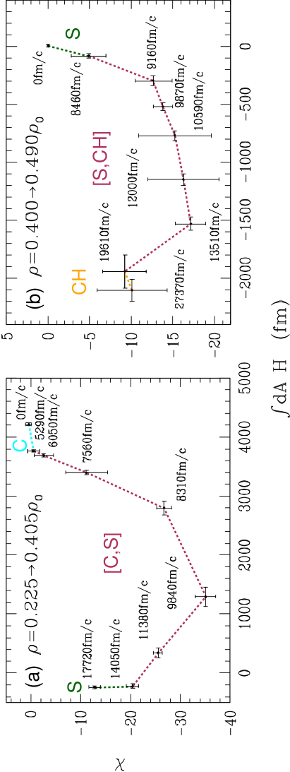
Figure 8: (Color) Time evolution of $\int_{\partial R}HdA$ and $\chi$ during the simulations. The data points and the error bars show, respectively, the mean values and the standard deviations in the range of the threshold density $\rho_{\rm th}=0.3$ – $0.5\rho_{0}$, which includes typical values for the nuclear surface. The panel (a) is for the transition from cylindrical (C) to slablike nuclei (S) and the panel (b) for the transition from slablike nuclei to cylindrical holes (CH). Transient states are shown as [C,S] and [S,CH] for each transition. Adapted from Ref. qmd_transition .

3.3 3. Formation of the Pasta Phases

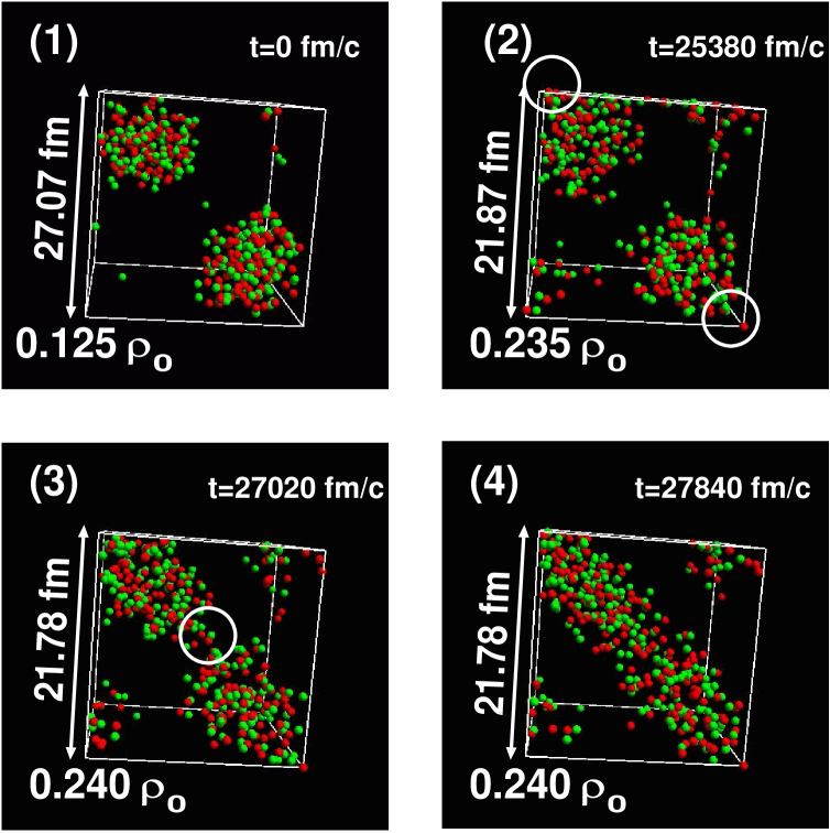
Figure 9: (Color) Snapshots of the transition process from the bcc lattice of spherical nuclei to the triangular lattice of rodlike nuclei (the whole simulation box is shown). The red particles show protons and the green ones neutrons. The box size is rescaled to be equal in this figure.

In closing the present article, let us briefly show our recent results of a study on the formation process of pasta nuclei from spherical ones; i.e., a transition from the phase with spherical nuclei to that with rodlike nuclei. Time evolution of the nucleon distribution in the transition process is shown in Fig. 9. The initial condition of this simulation is a nearly perfect bcc unit cell with 409 nucleons (202 protons and 207 neutrons) at $T\simeq 1$ MeV. We compressed the system in a similar way to that of the simulations explained in the previous section. The average rate of the density change in the present case is $\simeq$4.4$\times 10^{-6}\rho_{0}/$(fm$/c$). Since the two nuclei start to touch [see the circles in Fig. 9-(2)], the transition process completes within $\simeq 2500$ fm$/c$ and the rodlike nucleus is formed. The final state [Fig. 9-(4)] is a triangular lattice of the rodlike nuclei.

The present simulation has been performed using a rather small system; effects of the finite system size in this simulation should be examined. Detailed investigation of the transition using a larger system will be presented in a future publication future .

4 IV. Conclusion

We approached the two questions posed in Section I using the framework of QMD. According to the results of our simulations, our answer is strongly affirmative for both questions. The nuclear interaction used in our simulations shows generally reasonable properties at subnuclear densities not only for symmetric nuclear matter but also for neutron matter. This result also supports our conclusion.

References

- (1) J. Aichelin and H. Stöcker, Phys. Lett. B176, 14 (1986); J. Aichelin, Phys. Rep. 202, 233 (1991).
- (2) A. Akmal, V. R. Pandharipande and D. G. Ravenhall, Phys. Rev. C 58, 1804 (1998).
- (3) G. Baym, H. A. Bethe and C. J. Pethick, Nucl. Phys. A175, 225 (1971).
- (4) H. A. Bethe, Rev. Mod. Phys. 62, 801 (1990).
- (5) A. Burrows, S. Reddy and T. A. Thompson, Nucl. Phys. A, in press (astro-ph/0404432).
- (6) J. Carlson, J. Morales, Jr., V. R. Pandharipande and D. G. Ravenhall Phys. Rev. C 68, 025802 (2003).
- (7) F. Douchin and P. Haensel, Phys. Lett. B485, 107 (2000).
- (8) H. Feldmeier, Nucl. Phys. A515, 147 (1990); H. Feldmeier and J. Schnack, Prog. Part. Nucl. Phys. 39, 393 (1997).
- (9) D. Z. Freedman, Phys. Rev. D 9, 1389 (1974).
- (10) B. Friedman and V. R. Pandharipande, Nucl. Phys. A361, 502 (1981).
- (11) M. Hashimoto, H. Seki and M. Yamada, Prog. Theor. Phys. 71, 320 (1984).
- (12) C. J. Horowitz, M. A. Pérez-García, and J. Piekarewicz, Phys. Rev. C 69, 045804 (2004).
- (13) C. J. Horowitz, M. A. Pérez-García, J. Carriere, D. K. Berry, and J. Piekarewicz, Phys. Rev. C 70, 065806 (2004).
- (14) K. Iida, G. Watanabe and K. Sato, Prog. Theor. Phys. 106, 551 (2001); Erratum, ibid. 110, 847 (2003).
- (15) T. Kido, T. Maruyama, K. Niita and S. Chiba, Nucl. Phys. A663 & 664, 877c (2000).
- (16) M. Lassaut, H. Flocard, P. Bonche, P.H. Heenen and E. Suraud, Astron. Astrophys. 183, L3 (1987).
- (17) C. P. Lorenz, D. G. Ravenhall and C. J. Pethick, Phys. Rev. Lett. 70, 379 (1993).
- (18) G. Martinez-Pinedo, M. Liebendoerfer, D. Frekers, astro-ph/0412091.
- (19) T. Maruyama, K. Niita, K. Oyamatsu, T. Maruyama, S. Chiba and A. Iwamoto, Phys. Rev. C 57, 655 (1998).
- (20) T. Maruyama, T. Tatsumi, D. N. Voskresensky, T. Tanigawa, and S. Chiba, Phys. Rev. C 72, 015802 (2005).
- (21) K. Michielsen and H. De Raedt, Phys. Rep. 347, 461 (2001).
- (22) W. D. Myers, W. J. Swiatecki and C. S. Wang, Nucl. Phys. A436, 185 (1985).
- (23) K. Niita, in the Proceedings of the Third Simposium on “Simulation of Hadronic Many-body System”, A. Iwamoto et al., Eds., JAERI-conf. 96-009, 22 (1996) (in Japanese).
- (24) A. Ono, H. Horiuchi, T. Maruyama and A. Ohnishi, Prog. Theor. Phys. 87, 1185 (1992); Phys. Rev. Lett. 68, 2898 (1992).
- (25) K. Oyamatsu, Nucl. Phys. A561, 431 (1993).
- (26) C. J. Pethick and D. G. Ravenhall, Annu. Rev. Nucl. Part. Sci. 45, 429 (1995).
- (27) C. J. Pethick, D. G. Ravenhall and C. P. Lorenz, Nucl. Phys. A584, 675 (1995).
- (28) D. G. Ravenhall, C. D. Bennett and C. J. Pethick, Phys. Rev. Lett. 28, 978 (1972).
- (29) D. G. Ravenhall, C. J. Pethick and J. R. Wilson, Phys. Rev. Lett. 50, 2066 (1983).
- (30) K. Sato, Prog. Theor. Phys. 53, 595 (1975); ibid. 54, 1325 (1975).
- (31) P. J. Siemens and V. R. Pandharipande, Nucl. Phys. A173, 561 (1971).
- (32) O. Sjöberg, Nucl. Phys. A222, 161 (1974).
- (33) K. Sumiyoshi, K. Oyamatsu and H. Toki, Nucl. Phys. A595, 327 (1995).
- (34) G. Watanabe et al., to be published.
- (35) G. Watanabe and K. Iida, Phys. Rev. C 68, 045801 (2003).
- (36) G. Watanabe, K. Iida and K. Sato, Nucl. Phys. A676, 455 (2000); ibid. A687, 512 (2001); Erratum, ibid. A726, 357 (2003).
- (37) G. Watanabe, T. Maruyama, K. Sato, K. Yasuoka and T. Ebisuzaki, Phys. Rev. Lett. 94, 031101 (2005).
- (38) G. Watanabe, K. Sato, K. Yasuoka and T. Ebisuzaki, Phys. Rev. C 66, 012801(R) (2002); ibid. 68, 035806 (2003).
- (39) G. Watanabe, K. Sato, K. Yasuoka and T. Ebisuzaki, Phys. Rev. C 69, 055805 (2004).
- (40) G. Watanabe and H. Sonoda, to appear in “Soft Condnsed Matter: New Research”, ed. F. Columbus (cond-mat/0502515).
- (41) R. D. Williams and S. E. Koonin, Nucl. Phys. A435, 844 (1985).