The nuclear density of states and the role of the residual interaction

Abstract

We discuss the role of mean-field and moment methods in microscopic models for calculating the nuclear density of states (also known as the nuclear level density). Working in a shell-model framework, we use moments of the nuclear many-body Hamiltonian to illustrate the importance of the residual interaction for accurate representations.

1 Introduction: mean-fields and moments

“We all know that Art is not truth. Art is a lie that makes us realize the truth, at least the truth that is given to us to understand.” –Pablo Picasso.

If you want to model nuclear reactions in a hot, dense, neutron-rich environment, whether for astrophysics or for stockpile stewardship, you need to compute neutron capture rates where you have a thick forest of states or resonances[1]. If you want to compute statistical neutron capture using the Hauser-Feshbach formalism[2], you need the density of states, or the nuclear level density [3]. The nuclear level density is a challenge both experimentally and theoretically, because in essence one needs a reliable count of thousands or millions of states. The level density is generally quoted as being the most uncertain input into statistical capture calculations[1].

You don’t need information on each individual state or resonance; rather you need to average over many many states. The tools to average over the states, or rather over the nuclear many-body Hamiltonian, are mean-field methods and moment methods; later on we will discuss how moment methods can be considered as a generalization of mean-field methods.

A static mean-field picture is the basis for the most widely used approach to level densities, generalized Bethe Fermi gas models[4, 5]. Here one starts with a single-particle spectrum generated by a mean-field and derives the density of many-body states. The most sophisticated applications extract the single-particle spectrum from mean-field calculations, such as Skyrme Hartree-Fock[6]. The residual interaction is mostly ignored, although pairing interactions are included in part through a quasi-particle spectrum from Hartree-Fock-Bogoliubov, and corrections can be added for rotational motion, etc.. Although such approaches are simplest to use, the lack of consistent use of the entire residual interaction is arguably unsatisfactory.

The best framework to fully include the residual interaction is that of the interacting shell model, which uses a basis of many-body Slater determinants. For application to low-energy spectroscopy, one typically diagonalizes the nuclear Hamiltonian, but this is impractical for useful applications to the level density.

2 Spectral distribution methods

Nuclear statistical spectroscopy starts from the moments of the Hamiltonian. For example, in a finite space, most state densities of many-body systems with a two-body interaction tend toward a Gaussian shape [7] characterized by the first and second moments of the Hamiltonian. In most realistic cases the density has small but non-trivial deviations from a Gaussian, so one requires higher moments.

None of the formalism in this section is original; a thorough reference to statistical spectroscopy is Ref. [8], although some of our notation is different. Due to space limitations we give only a brief overview; for more careful discussion, readers are referred to our preprint[9].

We work in a finite model space ${\cal M}$ wherein the number of particles is fixed. If in ${\cal M}$ we represent the Hamiltonian as a matrix $\mathbf{H}$, then all the moments can be written in terms of traces. The total dimension of the space is $D=\mathrm{tr\,}\mathbf{1}$, and the average is $\langle\mathbf{O}\rangle=D^{-1}\mathrm{tr\,}\mathbf{O}.$ The first moment, or centroid, of the Hamiltonian is $\bar{E}=\langle\mathbf{H}\rangle;$ all other moments are central moments, computed relative to the centroid:

$$\mu^{(n)}=\langle(\mathbf{H}-\bar{E})^{n}\rangle\;\;.$$ (1)

The width $\sigma$ is given by $\sqrt{\mu^{(2)}}$, and one scales the higher moments by the width:

$$m^{(n)}=\frac{\mu^{(n)}}{\sigma^{n}}.$$ (2)

In addition to the centroid and the width, the next two moments have special names. The scaled third moment $m^{(3)}$ is the asymmetry, or the skewness.

It has long been realized that, rather than computing higher and higher moments of the total Hamiltonian, one could partition the model space into suitable subspaces and compute just a few moments in each subspace. In particular, if the space is partitioned using spherical shell-model configurations, that is, all states of the form $(0d_{5/2})^{4}(1s_{1/2})^{2}(0d_{3/2})^{2}$, etc., then it is possible to derive expressions for the configuration moments directly in terms of the single-particle energies and two-body matrix elements, without constructing any many-body matrix elements.

We use $\alpha,\beta,\gamma,\ldots$ to label subspaces. Let

$$P_{\alpha}=\sum_{i\in\alpha}\left|i\right\rangle\left\langle i\right|$$ (3)

be the projection operator for the $\alpha$-th subspace. One can introduce partial or configuration densities,

$$\rho_{\alpha}(E)=\mathrm{tr}\,P_{\alpha}\delta(E-\mathbf{H}).$$ (4)

The total level density $\rho(E)$ is just the sum of the partial densities.

Now we define configuration moments: the configuration dimension is $D_{\alpha}={\rm tr\,}P_{\alpha}$, the configuration centroid is $\bar{E}_{\alpha}=D_{\alpha}^{-1}{\rm tr\,}P_{\alpha}\mathbf{H},$ while the configuration width $\sigma_{\alpha}$ and configuration asymmetry $m_{\alpha}^{(3)}$ are defined in the obvious ways.

One important result from spectral distribution theory is that the configuration centroids depend entirely upon the single-particle energies and the monopole-monopole part of the residual interaction[10]. The monopole interaction is attributed to mean-field and saturation properties of the nuclear interaction. One can subtract out the monopole interaction exactly, which sets the centroids to zero but leaves the widths unchanged; such a monopole-subtracted interaction is referred to as a “traceless” interaction. For some more information on computing the monopole interaction, see the references [8, 9].

3 First moments: the mean field

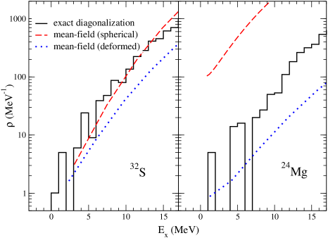
Figure 1: Comparison of exact level density (from complete diagonalization of shell-model Hamiltonian) with Fermi gas model, using spherical (dashed lines) mean-field or deformed (dotted) mean-field. Left: ³²S. Right: ²⁴Mg. Both are computed in $sd$-shell with USD interaction.

The thermodynamic approach to the density of states is to note that the partition function $Z$ is the Laplace transform of the density, $Z(\beta)=\int e^{-\beta E}\rho(E)dE$. The inverse Laplace transform is accomplish through either a saddle-point approximation [4, 11] or maximum entropy [12]. The many-body partition function can in principle be computed from the full Hamiltonian, including the residual interaction, using path integrals[11, 12], but the integrals must be evaluated through Monte Carlo sampling and in order to avoid the sign problem, only a restricted class of Hamiltonians can be used[13].

Instead, as mentioned in the introduction, the standard approach is to approximate the many-body partition function using non-interacting particles in a mean field[4]. That is,

$$\ln Z(\alpha,\beta)=\int g(\epsilon)\ln\left(1+\exp(\alpha-\beta\epsilon)\right)d\epsilon$$ (5)

where $g(\epsilon)=\sum_{i}\delta(\epsilon-\epsilon_{i})$ is the single-particle density of states, $\{\epsilon_{i}\}$ are the mean-field single-particle energies, and $\alpha$ is proportional to the chemical potential. The excitation energy and the particle number are set through the derivatives of $\ln Z$ with respect to $\beta$ and $\alpha$, respectively.

For an example of applying this method, Goriely et al[6] extract single-particle energies from Skyrme Hartree-Fock calculations and use it to estimate level densities throughout the nuclear landscape. To illustrate this, we consider a nontrivial model system, a finite-basis interacting shell model, where we can compare the “true” density of states (from numerical diagonalization of the many-body Hamiltonian) with approximate methods. We work in the $sd$-shell and lower $pf$-shell where there are sufficiently few number of levels (a few thousand) so that one can carry out the full diagonalization using the shell model codes OXBASH[14] and REDSTICK[15]. The Hartree-Fock calculations were done using a shell-model based code, SHERPA, used to test the random phase approximation in exactly the same way[16].

Two sample results are shown in Fig. (1), for ³²S and ²⁴S, with valence nucleons in the $sd$-shell using the so-called universal sd-shell (USD) interaction[17]. The Fermi gas calculations are done exactly according to the prescription with no corrections.

One sees that for a spherical nucleus, ³²S, the mean-field Fermi gas calculation works extremely well for such a simple prescription. ²⁴Mg, which is deformed, is much more problematic. For both nuclides we computed the single-particle energies for both spherical and deformed mean-fields. Neither yield a very good description for ²⁴Mg (and for other deformed nuclei), and indeed in practical applications[6] one typically includes “rotational enhancement” and other corrections.

The sample calculation in Fig. (1) is crude and should not be taken as an indictment of Fermi gas model calculations; lacking other approaches, they are the best game in town. The above exercise is intended to inculcate a desire to go beyond the mean-field to include the residual interaction.

4 Second moments: the residual interaction

To go beyond the mean field and include the residual interaction, we turn to the concepts of Section 2. In particular we write the total density as a sum of configuration densities. But how do we model the configuration densities?

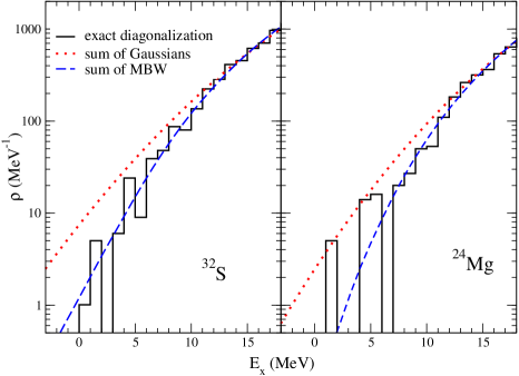
Figure 2: Comparison of exact level density (from complete diagonalization of shell-model Hamiltonian) with sum of Gaussians.

In this section we approximate the configuration densities as Gaussians[18], with the average and width given by the configuration centroid and width, respectively. We remind the reader that the configuration centroids arise from the mean-field, while the width, or second moment, reflects the strength of the residual interaction. Elsewhere we show that the configuration width is approximately constant[9], at least within a major oscillator shell.

The results for ³²S and ²⁴Mg are plotted in Fig. (2) (dotted line). While for the latter this is an improvement over the zeroth order mean-field results as seen in Fig 1, it still does poorly at low energy. (For some nuclides, not shown here, the Gaussian approximation is sufficient[18].) Therefore we must go beyond second moments and go to third moments.

5 Third moments: collectivity

First configuration moments (centroids) reflect the mean-field; second moments (widths) reflect the overall strength of the residual interaction. Third moments, we claim, are indicative of collectivity. The argument follows from simple pictures of collectivity, whereby one has a single collective state pushed down or up in energy relative to the remaining degenerate noncollective states. Because of the inherent asymmetry one has a nontrivial third moment. This is distinct from the spreading width (second moment) which, in simplest terms, spreads out the states symmetrically. Calculations of well-known collective interactions, such as $Q\cdot Q$, show strong persistent third moments [9]. The real situation is more subtle than this, but as a simple paradigm of level densities this argument suffices.

To include third moments in our models for partial densities, we need something beyond Gaussians for the configuration densities. Many suggestions have been made, such as Gram-Charlier expansions[8], Cornish-Fisher expansions[19], or binomials[20]. We use a modified Breit-Wigner (MBW) form,

$$\rho_{\mathrm{MBW}}(E)=\frac{1}{W^{3}}\frac{(E_{\mathrm{max}}-E)^{2}(E-E_{\mathrm{min}})^{2}}{(E-E_{0})^{2}+W^{2}}$$ (6)

which has several advantageous characteristics, including positive-definite on the interval $E_{\mathrm{min}}<E<E_{\mathrm{max}}$, and exact analytic moments. The four parameters of Eq. (6) can be fitted to reproduce the first four configuration moments.

Fig. (2) compares exact calculations of ³²S and ²⁴Mg with a sum of MBW configuration densities (dashed line), which are significant improvements over the sum of Gaussians (dotted lines). For this calculation we computed the third and fourth configuration moments from the many-body Hamiltonian matrix, generated using the REDSTICK shell model code. In principle, one can compute the moments directly from the two-body matrix elements[8] but we have found apparently discrepancies between the published formulas and direct calculation, which we have been unable to resolve so far. A more serious problem is that even if one would able to compute the third and fourth moments directly, they are very time-consuming for large spaces. Two options suggest themselves. First, as seen in Fig. (2), at moderate excitation energy the Gaussian and MBW curves converge, suggesting that one only needs 3rd and 4th moments at lower energy. This further supports our suggestion to think of the third moment as a sign of collectivity. Second, at least part of the asymmetry in fact arises from the mean-field, which leads to approximate formulas for the asymmetry[9]. Unpublished results suggest these approximations are partially but not wholly successful, so more work is required.

6 Comparision with experiment

So far we have only compared models against models, which in our case means validating an approximate approach against a more detailed calculation, using exactly the same input. But we need to compare against real experimental data. While mean-field/Fermi gas models have been compared extensively against experiment [5, 6], moments methods have rarely been compared against experiment[21].

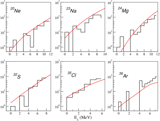
Figure 3: Comparison of experimental state densities (binned) of $sd$ shell nuclides against our calculations, including factor-of-two for opposite parity states.

Although important technical issues remain (such as accurate and efficient calculation of third and fourth moments when needed, and determination of the ground state energy), for large-scale application of moments methods the most significant issue is the choice of interaction. Most shell-model interactions are adjusted for relatively small model spaces; but believeable calculations of the density of states requires so-called “intruder” configurations such as those of opposite parity. This will be the major focus of subsequent work.

Nonetheless we can perform preliminary calculations. We show them in Figs. (3) ($sd$-shell using the USD interaction[17]) and (4) ($pf$-shell using GXPF1[23]). The experimental data are taken from individual states obtained from the Reference Input Library of the Nuclear Data Services site [22]. The third and fourth moments were computed in an approximate fashion. The ground state energies were computed either using REDSTICK or via Hartree-Fock + RPA (the code SHERPA)[16]. As the model spaces were for a single parity, we multiplied by a factor of 2 to estimate the opposite parity contribution. This is a crude approach and one which needs refinement; there have been many papers examining the relative contribution of opposite parity states to the level density[24]. We do well for $sd$-shell nuclides and, in the $pf$ shell, for ⁴⁸Ti and ⁴⁵Sc, but not so well for ⁵¹V and ⁵²Cr. While our crude treatment of parity may be partly at fault, the most likely culprit is the interaction, and in particular the monopole (mean-field) structure of the interaction.

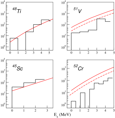
Figure 4: Same as Fig. 3, but in $pf$ shell. Dashed lines on ⁵²V and ⁵²Cr are for normal parity states only.

7 Conclusions

We have reviewed applying spectral distribution methods to the nuclear density of states. To guide the reader, we linked the first moment to Hartree-Fock energies and effective single-particle energies, which form the basis for mean-field Fermi gas calculations. Use of the residual interaction lead to higher moments, in particular the second and third moments, which we interpret as spreading widths and collectivity, respectively.

Finally, we can suggest a revision of Picasso’s quote:

We all know that models are not reality. Models are lies that makes us understand reality, at least that part of reality that is given to us to understand.

This work is supported by grant DE-FG52-03NA00082 from the Department of Energy /National Nuclear Security Agency. CWJ acknowledges helpful conversations with Dr. W. E. Ormand.

References

- [1] T. Rauscher, F.-K. Thielemann, and K.-L. Kratz, Phys. Rev. C 56, 1613 (1997)
- [2] W. Hauser and H. Feshbach, Phys. Rev. 87, 366 (1952).
- [3] The state density includes degeneracies, while the level density does not. For applications it is important to distinguish between them, but, following colloquial usage, we use the terms interchangeably. Except for -projected level densities, everything else we discuss is technically a state density.
- [4] H. A. Bethe, Phys. Rev. 50, 332 (1936); A. Gilbert and A. G. W. Cameron, Can. J. Phys. 43, 1446 (1965); A. Bohr and B. R. Mottelson, Nuclear Structure, Vol. I: Single-particle Motion, Appendix 2B (W. A. Benjamin, Boston, 1969).
- [5] W. Dilg, W. Schantl, H. Vonach, and M. Uhl, Nucl. Phys. A217, 269 (1973).
- [6] S. Goriely, Nucl. Phys. A 605, 28 (1996); P. Demetriou and S. Goriely, Nucl. Phys. A 695, 95 (2001).
- [7] K. K. Mon and J. B. French, Ann. Phys. 95, 90 (1975); V. K. B. Kota, Z. Phys. A 315, 91 (1984).
- [8] S. S. M. Wong, Nuclear Statistical Spectroscopy (Oxford University Press, New York, 1986).
- [9] E. Terán and C. W. Johnson, arXiv:nucl-th/0508040.
- [10] J. Duflo and A. P. Zuker, Phys. Rev. C 67, 054309 (2003).
- [11] H. Nakada and Y. Alhassid, Phys. Rev. Lett. 79, 2939 (1997); H. Nakada and Y. Alhassid, Phys. Lett. B 436, 231 (1998).
- [12] W. E. Ormand, Phys. Rev. C 56, R1678 (1997).
- [13] G. H. Lang, C. W. Johnson, S. E. Koonin, and W. E. Ormand, Phys. Rev. C 48, 1518 (1993).
- [14] B. A. Brown, A. Etchegoyen, and W. D. M. Rae, Michigan State University Cyclotron Report No. 524 (1984).
- [15] W. E. Ormand, private communication.
- [16] I. Stetcu and C. W. Johnson, Phys. Rev. C 66, 034301 (2002).
- [17] B. H. Wildenthal, Prog. Part. Nucl. Phys. 11, 5 (1984).
- [18] M. Horoi, J. Kaiser, and V. Zelevinsky, Phys. Rev. C 67, 054309 (2003).
- [19] V. K. B. Kota, V. Potbhare, and P. Shenoy, Phys. Rev. C 34, 2330 (1986).
- [20] A. P. Zuker, Phys. Rev. C 64, 021303(R) (2001); C. W. Johnson, J. Nabi, W. E. Ormand, arXiv:nucl-th/0105041.
- [21] P.Huang, S. M. Grimes, and T. N. Massey , Phys Rev C 62, 024002 (2000).
- [22] URL http://www-nds.iaea.org/.
- [23] M. Honma, T. Otsuka, B.A. Borwn, and T. Mizusaki, Phys. Rev. C 69, 034335 (2004).
- [24] U. Agvaanluvsan, G. E. Mitchell, J. F. Shriner, Jr., and M. Pato Phys. Rev. C 67, 064608 (2003);Y. Alhassid, G. F. Bertsch, S. Liu, and H. Nakada Phys. Rev. Lett. 84, 4313 (2000).