Analysis of the ⁶He $\beta$ decay into the $\alpha+d$ continuum within a three-body model

Abstract

The $\beta$-decay process of the ⁶He halo nucleus into the $\alpha+d$ continuum is studied in a three-body model. The ⁶He nucleus is described as an $\alpha+n+n$ system in hyperspherical coordinates on a Lagrange mesh. The convergence of the Gamow-Teller matrix element requires the knowledge of wave functions up to about 30 fm and of hypermomentum components up to $K=24$. The shape and absolute values of the transition probability per time and energy units of a recent experiment can be reproduced very well with an appropriate $\alpha+d$ potential. A total transition probability of $1.6\times 10^{-6}$ s^-1 is obtained in agreement with that experiment. Halo effects are shown to be very important because of a strong cancellation between the internal and halo components of the matrix element, as observed in previous studies. The forbidden bound state in the $\alpha+d$ potential is found essential to reproduce the order of magnitude of the data. Comments are made on $R$-matrix fits.

I Introduction

The discovery of light halo nuclei with very large matter radii near the neutron drip line tan96 inspired detailed studies of the structure of these quantum systems. The large radii are interpreted as arising from an extended spatial density of a few neutrons han87 ; zhu91 . The static properties of the halo nuclei do not provide a complete picture of their structure and especially of the halo extension. Few observables directly probe the probability density at very large distances.

The $\beta$ decay with emission of a deuteron, also known as $\beta$ delayed deuteron decay, is energetically possible for nuclei with a two-neutron separation energy $S_{2n}$ smaller than 3 MeV. This property is typical of halo nuclei. The measurement of the spectrum shape for this decay process offers a unique opportunity of probing halo properties at large distances. The $\beta$ decay of ⁶He into $\alpha$ and a deuteron has been observed in several experiments rii90 ; bor93 ; ABB02 . The branching ratio is much smaller than expected from simple $R$-matrix rii90 , two-body Pierre92 , and three-body zhu93 models. Various experimental values of this branching ratio have been obtained, i.e., $(2.8\pm 0.5)\times 10^{-6}$ rii90 , $(7.6\pm 0.6)\times 10^{-6}$ bor93 , and $(1.9\pm 0.8)\times 10^{-6}$ ABB02 , for a deuteron cutoff energy of about 350 keV. The latest result ABB02 is a factor of 4 smaller than the result of Ref. bor93 which served as reference for most theoretical papers.

A semi-microscopic study BSD94 of the process has been able to explain that the low value of the branching ratio is the result of a cancellation between the ”internal” and ”external” parts of the Gamow-Teller matrix element. The overlaps of the ⁶He ground state and $\alpha+d$ scattering wave functions in the internal ($R<5$ fm) and external ($R>5$ fm) regions have very close magnitudes but opposite signs. It is clear that the external part of the Gamow-Teller matrix element reflects properties of the halo structure of the ⁶He nucleus. An improved microscopic wave function of ⁶He confirmed this interpretation VSO94 . It was also confirmed by a fit in the $R$-matrix framework bar94 which yields a satisfactory description of the deuteron spectrum shape and branching ratio of Ref. bor93 . A fully microscopic description of the $\beta$ decay of the ⁶He nucleus to the ⁶Li ground state and to the $\alpha+d$ continuum cso94 was performed in a dynamical microscopic cluster model with consistent fully antisymmetrized wave functions for the initial bound state and the final scattering state. This model provided a reasonable agreement with the data of Ref. bor93 . Without any fitted parameter, those data were underestimated by about a factor of 2. Hence, the same microscopic results now overestimate the recent data of Ref. ABB02 by a similar factor.

Since new data ABB02 with much better statistics which provide an even lower branching ratio are now available, it is timely to reexamine the interpretation of the $\beta$ delayed deuteron decay. Improving significantly the microscopic model of Ref. cso94 is not yet possible. We prefer thus to base our discussion on an $\alpha+n+n$ three-body model. Accurate wave functions of ⁶He are available in hyperspherical coordinates DDB03 . A previous calculation based on the same model zhu93 contains several limitations which led to a significant overestimation of the data of Ref. bor93 : the calculations were restricted to small values of the hypermomentum, $K=0$ and 2, and the halo description may not have been sufficiently extended.

The aim of the present work is the determination of the deuteron spectrum shape and branching ratio for the $\beta$ decay of the ⁶He halo nucleus into $\alpha+d$ with an accurate treatment of the ⁶He wave function in an $\alpha+n+n$ three-body cluster model. For the description of the structure of the ⁶He nucleus, we use the hyperspherical harmonics method on a Lagrange mesh BH-86 ; DDB03 which yields an accurate solution in this model. The $\alpha+d$ scattering wave function is treated as factorized into a deuteron wave function and a nucleus-nucleus relative wave function. We will choose several versions of the central interaction potential between $\alpha$ and $d$: a deep Gaussian potential dub94 which fits both the $s$-wave phase shift and the binding energy of the ⁶Li ground state (1.473 MeV), and potentials obtained by folding the $\alpha+N$ potential of Voronchev et al. vor95 . For the sake of comparison we will also perform a calculation with a repulsive $\alpha+d$ potential which was used in Ref. zhu93 .

In Sec. II, the formalism of the $\beta$-decay process of the ⁶He nucleus into the $\alpha+d$ continuum is presented. The potentials and the corresponding three-body hyperspherical and two-body scattering wave functions are also described. In Sec. III, we discuss the obtained numerical results in comparison with experimental data. Finally conclusions are given in Sec. IV.

II Model

II.1 ⁶He wave function

The initial three-body wave function is expressed in hyperspherical coordinates. Particles 1 and 2 are the nucleons and 3 is the $\alpha$ cluster. A set of Jacobi coordinates for the three particles with mass numbers $A_{1}=1$, $A_{2}=1$, and $A_{3}=4$ is defined as

$$\mbox{\boldmath$x$}=\sqrt{\mu_{12}}\mbox{\boldmath$r$},\hskip 28.45274pt\mbox{\boldmath$y$}=\sqrt{\mu_{(12)3}}\mbox{\boldmath$R$},$$ (1)

where $\mbox{\boldmath$r$}=\mbox{\boldmath$r$}_{2}-\mbox{\boldmath$r$}_{1}$ and $\mbox{\boldmath$R$}=\mbox{\boldmath$r$}_{3}-\mbox{$\frac{1}{2}$}(\mbox{\boldmath$r$}_{1}+\mbox{\boldmath$r$}_{2})$. The (dimensionless) reduced masses are given by $\mu_{12}=1/2$ and $\mu_{(12)3}=4/3$. Equations (1) define six coordinates which are transformed to the hyperspherical coordinates by

$$\rho^{2}=x^{2}+y^{2},\hskip 28.45274pt\alpha=\arctan(y/x),$$ (2)

where $\alpha$ varies between 0 and $\pi/2$. With the angular variables $\Omega_{x}=(\theta_{x},\varphi_{x})$ and $\Omega_{y}=(\theta_{y},\varphi_{y})$, Eqs. (2) define a set of hyperspherical coordinates. These coordinates are known to be well adapted to the three-body Schrödinger equation.

With the notation $\Omega_{5}=(\alpha,\Omega_{x},\Omega_{y})$, the wave function reads DDB03

$$\Psi^{00+}_{{}^{6}{\rm He}}(\rho,\Omega_{5})=\rho^{-5/2}\sum_{l_{x}l_{y}LSK}{\chi}^{0+}_{l_{x}l_{y}LSK}(\rho){\cal Y}^{00}_{l_{x}l_{y}LSK}(\Omega_{5}),$$ (3)

where $l_{x}$ and $l_{y}$ are the orbital momenta associated with the Jacobi coordinates $x$ and $y$, respectively, ${\cal Y}^{JM}_{l_{x}l_{y}LSK}$ are hyperspherical harmonics, and ${\chi}^{J\pi}_{l_{x}l_{y}LSK}$ are hyperradial functions.

The ⁶He ground state wave function contains components with total intrinsic spin $S=0$ and 1. The total orbital momentum $L$ is equal to $S$. Because of the positive parity, $l_{x}+l_{y}$ is even and the sums in Eq. (3) and in the following run over even $K$ values only.

II.2 $\alpha+d$ wave function

For the scattering state, we assume an expression factorized into the deuteron ground-state wave function and an $\alpha+d$ scattering wave function derived from a potential model. The deuteron spin 1 and positive parity allow $S$ and $D$ components. Here, we neglect the small $D$ component of the deuteron.

Below, we only need the $1^{+}$ component of the $\alpha+d$ scattering function which reads

$$\Psi^{1M+}_{\alpha d}(E,\mbox{\boldmath$r$},\mbox{\boldmath$R$})=\Psi_{d}(\mbox{\boldmath$r$})\psi_{\alpha d}(E,\mbox{\boldmath$R$}).$$ (4)

where $r$ and $R$ are here the deuteron and $\alpha+d$ relative coordinates, respectively. The spatial part of the deuteron wave function $\Psi_{d}$ is written as

$$\psi_{d}(\mbox{\boldmath$r$})=r^{-1}u_{d}(r)Y_{00}(\Omega_{x}).$$ (5)

The spatial part of the $\alpha+d$ $s$-wave function is factorized as

$$\psi_{\alpha d}(E,\mbox{\boldmath$R$})=R^{-1}u_{E}(R)Y_{l0}(\Omega_{y}).$$ (6)

The radial scattering wave function $u_{E}$ has the asymptotic behavior,

$$u_{E}(R)\mbox{$\mathop{\rightarrow}\limits_{R\rightarrow\infty}$}\cos\delta_{0}(E)F_{0}(kR)+\sin\delta_{0}(E)G_{0}(kR),$$ (7)

where $k$ is the wave number of the relative motion, $F_{0}$ and $G_{0}$ are Coulomb functions, and $\delta_{0}(E)$ is the $s$-wave phase shift at energy $E$.

The radial functions $u_{E}$ are calculated with effective $\alpha+d$ potentials. Some among the potentials $V_{\alpha d}(R)$ we are using are obtained by folding an $\alpha+N$ potential $V_{\alpha N}(r)$. They are given by the equation

$$V_{\alpha d}(R)=\langle\psi_{d}(\mbox{\boldmath$r$})\mid V_{\alpha n}(|\mbox{\boldmath$R$}+\mbox{$\frac{1}{2}$}\mbox{\boldmath$r$}|)+V_{\alpha p}(|\mbox{\boldmath$R$}-\mbox{$\frac{1}{2}$}\mbox{\boldmath$r$}|)\mid\psi_{d}(\mbox{\boldmath$r$})\rangle,$$ (8)

where the integration is performed over the radial and angular parts of variable $r$.

II.3 Transition probability per time and energy units

For the $\beta$-decay process

$${}^{6}{\rm He}\to\alpha+d+{\rm e}^{-}+\bar{\nu},$$ (9)

the transition probability per time and energy units is given by BD-88

$$\frac{dW}{dE}=\frac{m_{e}c^{2}}{\pi^{4}v\hbar^{2}}G_{\beta}^{2}f(Q-E)B_{\rm GT}(E),$$ (10)

where $m_{e}$ is the electron mass, $v$ and $E$ are the relative velocity and energy in the center of mass system of $\alpha$ and deuteron, and $G_{\beta}=2.996\times 10^{-12}$ is the dimensionless $\beta$-decay constant wil82 . The Fermi integral $f(Q-E)$ depends on the kinetic energy $Q-E$, available for the electron and antineutrino. The mass difference $Q$ between initial and final particles is 2.03 MeV.

Between an initial state with isospin $T=1$ and a final state with isospin $T=0$, Gamow-Teller transitions are allowed. The reduced transition probability reads

$$B_{\rm GT}(E)=12\lambda^{2}\sum_{M}|\langle\Psi^{1M+}_{\alpha d}(E)|\sum_{j=1}^{2}t_{j-}s_{jz}|\Psi^{00+}_{{}^{6}{\rm He}}\rangle|^{2},$$ (11)

where $\lambda=1.268\pm 0.002$ is the ratio of the axial-vector to vector coupling constants dub90 , $\Psi^{1M+}_{\alpha d}(E)$ is the wave function (4) of the final $\alpha+d$ system, and $\Psi^{00+}_{{}^{6}{\rm He}}$ is the wave function (3) of ⁶He. The operators $\mbox{\boldmath$s$}_{j}$ and $\mbox{\boldmath$t$}_{j}$ are the spin and isospin operators of particle $j$, respectively.

Since the total orbital momentum and parity are conserved, only the $l=0$ partial scattering wave contributes. Hence, only the initial $L=S=0$ component of ⁶He can decay to $\alpha+d$. It is convenient to express the Gamow-Teller matrix element with the help of an effective wave function BSD94 ,

$$\psi_{\rm eff}(\mbox{\boldmath$R$})=\int\psi_{d}(\mbox{\boldmath$r$})\psi^{0}_{{}^{6}{\rm He}}(\mbox{\boldmath$r$},\mbox{\boldmath$R$})d\mbox{\boldmath$r$}.$$ (12)

In this expression, $\psi^{0}_{{}^{6}{\rm He}}(\mbox{\boldmath$r$},\mbox{\boldmath$R$})$ is the spatial part of the $S=0$ component of the ⁶He wave function. The reduced transition probability can be written as

$$B_{\rm GT}(E)=6\lambda^{2}\left[\int\psi_{\alpha d}(E,\mbox{\boldmath$R$})\psi_{\rm eff}(\mbox{\boldmath$R$})d\mbox{\boldmath$R$}\right]^{2}.$$ (13)

Since only $l_{x}=l_{y}=L=S=0$ contributes, let us define

$$Z_{K}(r,R)=\rho^{-5/2}\chi_{0000K}(\rho)\mathcal{N}_{K}P_{K/2}^{1/2,1/2}(\cos 2\alpha),$$ (14)

where $\mathcal{N}_{K}$ is a normalisation factor coming from ${\cal Y}^{00}_{0000K}$ given by Eq. (10) of Ref. DDB03 and $P_{K/2}^{1/2,1/2}$ is a Jacobi polynomial abr70 . After integration over all angles, the reduced transition probability (13) becomes

$$B_{\rm GT}(E)=6\lambda^{2}\left[\sum_{K}\int_{0}^{\infty}u_{E}(R)u^{(K)}_{\rm eff}(R)dR\right]^{2}.$$ (15)

It involves the $K$-dependent effective functions

$$u^{(K)}_{\rm eff}(R)=R\int_{0}^{\infty}Z_{K}(r,R)u_{d}(r)rdr,$$ (16)

the sum of which forms the radial part of $\psi_{\rm eff}(\mbox{\boldmath$R$})$.

III Results and discussion

III.1 Conditions of the calculation

The central Minnesota interaction thom77 reproduces the deuteron binding energy and fairly approximates the low-energy nucleon-nucleon scattering properties. The deuteron wave function $\psi_{d}$ is calculated over a Lagrange-Laguerre mesh involving 40 mesh points and a scaling parameter $h=0.25$ fm (see Ref. DDB03 for details). An energy $E_{d}=-2.202$ MeV is obtained. The calculations are done with $\hbar^{2}/2m_{N}=20.734$ MeV fm².

The initial $\alpha+n+n$ bound state is calculated as explained in Ref. DDB03 . The number of components is limited to $K_{\rm max}=24$. The same nucleon-nucleon interaction is used, i.e., the Minnesota interaction with an exchange parameter $u=1$. The $\alpha+N$ potential is however different from the one employed in Ref. DDB03 . Here we employ the $\alpha+N$ potential of Voronchev et al. vor95 with a multiplicative factor 1.035 in order to reproduce the ⁶He binding energy. This change of interaction is motivated by the fact that we want to use the same interaction for the derivation of the $\alpha+d$ folding potential. The renormalization factor slightly affects the ⁵He properties. For the $3/2^{-}$ resonance, the original potential of Ref. vor95 provides an energy $E_{R}=0.80$ MeV and a width $\Gamma=0.75$ MeV, in nice agreement with experiment. Introducing the renormalization factor provides $E_{R}=0.55$ MeV and $\Gamma=0.40$ MeV, but does not affect the unstable nature of the resonance.

Since the valence neutron and proton in the ⁶Li nucleus belong to the $0p_{3/2}$ subshell, we use the $p$-wave $\alpha+N$ potential of Ref. vor95 when deriving the $\alpha+d$ folding potential by using Eq. (8). For the $s$ wave, this potential yields two bound states for ⁶Li with energies $E_{0}=-19.87$ MeV and $E_{1}=-0.83$ MeV, respectively. The first one is forbidden by the Pauli principle and the second one is underbound compared with the experimental ground-state energy $E_{\rm exp}=-1.473$ MeV. The $\alpha+N$ potential of Kanada et al. KKN79 employed in Ref. DDB03 does not yield an $\alpha+d$ folding potential with a physical bound state in the $s$ wave.

The numerical calculations of the Gamow-Teller matrix elements are done with several potentials. (i) The simple Gaussian attractive potential $V_{a}=-76.12\exp(-0.2r^{2})$ dub94 simultaneously provides the correct ⁶Li binding energy (together with a forbidden state) and a fair fit of the low-energy experimental phase shifts. (ii) The folding potential does not reproduce the ⁶Li ground-state energy. Therefore, we multiply the central part of the original $\alpha+N$ potential by a factor $f_{1}=1.068$. The $\alpha+d$ folding potential $V_{f1}$ moves the physical state to $E_{1}=-1.470$ MeV. (iii) The folding potential $V_{f1}$ does not have the same quality of phase shift description as the simple Gaussian potential $V_{a}$. Therefore, we also choose another multiplicative factor $f_{2}=1.15$ for the folding potential $V_{f2}$, which gives a stronger binding for the ⁶Li ground state, $E_{1}=-2.386$ MeV. (iv) Finally, for the sake of comparison with Ref. zhu93 , we also perform a calculation with their Woods-Saxon repulsive potential ($V_{r}$). Of course, it does not bind ⁶Li.

The $s$-wave phase shifts for the different $\alpha+d$ potentials are compared in Fig. 1 with the results of phase-shift analyses GSK75 ; JGK83 . The description of the $\alpha+d$ phase shift is poorest for the repulsive potential. Fair, almost identical, phase shifts are obtained with $V_{a}$ and $V_{f2}$.

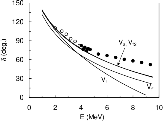
Figure 1: $s$-wave phase shifts obtained with different $\alpha+d$ potentials: attractive Gaussian potential $V_{a}$ dub94 , folding potentials $V_{f1}$ and $V_{f2}$ (see text), and repulsive Woods-Saxon potential $V_{r}$ zhu93 . Phase shifts are taken from analyses of experimental data in Refs. GSK75 (open dots) and JGK83 (full dots).

In Eqs. (16) and (8), the integration over $r$ is done by using the Gauss-Laguerre quadrature consistent with the Lagrange mesh. This ensures numerical convergence for the transition probability. The integration over variable $R$ in Eq. (15) is performed with the simple trapezoidal rule with a step 0.05 fm. Later we show that with this choice of step, convergent results for the transition probability are obtained with 600 points, which corresponds to a maximal $\alpha+d$ relative distance $R_{\rm max}=30$ fm.

We have also calculated the Gamow-Teller matrix element for the $\beta$ decay to the ⁶Li ground state. For this calculation, we replace wave function $\Psi^{1+}_{\alpha d}(E)$ in Eq. (11) by the $\alpha+n+p$ wave function of the ⁶Li ground state obtained with the same nuclear interactions as for ⁶He. The result $B_{\rm GT}=4.489\lambda^{2}$ is about 5 % below the experimental value $B_{\rm GT}^{(\rm exp)}=4.745\lambda^{2}$. With the potential of Ref. KKN79 for the ⁶He description, we find $B_{\rm GT}=4.636\lambda^{2}$. The sensitivity with respect to the ⁶He wave function is therefore small.

III.2 Effective wave functions and their integrals

In order to analyze the cancellation effects in the Gamow-Teller matrix element for the $\beta$ delayed deuteron decay, we display in Fig. 2 the integrals

$$I_{E}^{(K)}(R)=\int_{0}^{R}u_{E}(R^{\prime})u_{\rm eff}^{(K)}(R^{\prime})dR^{\prime}$$ (17)

at the $\alpha+d$ relative energy $E=1$ MeV for different $K$ values.

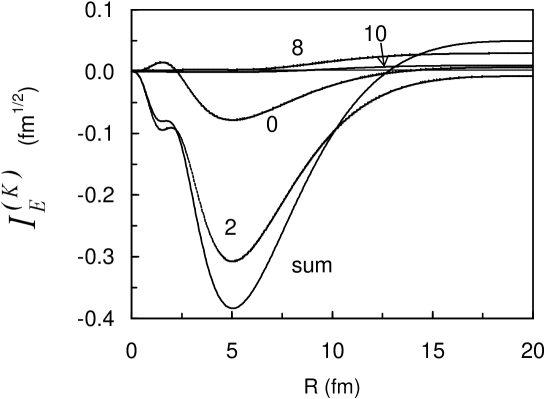
Figure 2: Integrals $I_{E}^{(K)}(R)$ [Eq. 17)] at the energy $E=1$ MeV for the $\alpha+d$ potential of Ref. dub94 and different $K$ values with $K_{\rm max}=24$ and $R_{\rm max}=30$ fm. The other components would hardly be visible at the scale of the figure.

They are calculated by using the $\alpha+d$ potential of Ref. dub94 . The reduced transition probability is given by the limit

$$B_{\rm GT}(E)=6\lambda^{2}\left[\lim_{R\to\infty}\sum_{K}I_{E}^{(K)}(R)\right]^{2}.$$ (18)

¿From Fig. 2, one can see that at large $R$ values the dominant contribution to $\sum_{K}I_{E}^{(K)}$ for all $K$ values up to $K_{\rm max}$ comes from the $K=2$ and $K=8$ components. Components for $K=4$ and $K=6$ as well as for $K\geq 12$ are not visible with the linear scale of Fig. 2. Although the $K=0$ component is rather important around $R=5$ fm, it is suppressed at large $R$ values even more than the $K=10$ component.

To understand this interesting effect, we display different components $u_{\rm eff}^{(K)}(R)$ of the effective wave function as dotted lines in Fig. 3. The full line represents the sum

$$u_{\rm eff}(R)=\sum_{K=0}^{K_{\rm max}}u_{\rm eff}^{(K)}(R).$$ (19)

In Fig. 3, we also show the $\alpha+d$ scattering $s$-wave function $u_{E}$ for $E=1$ MeV. It is important to note that this function keeps a constant sign in the interval 5-19 fm. This constant-sign interval is even broader for smaller values of $E$. The $K=0$ and $K=2$ components are dominant at all relative distances $R$. They exhibit a maximum below 5 fm. One observes that $u_{\rm eff}^{(0)}$ keeps a constant sign over the whole region while $u_{\rm eff}^{(2)}$ changes sign at $R\approx 2$ fm.

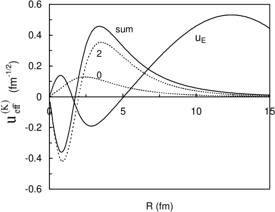
Figure 3: Effective wave functions $u_{\rm eff}^{(K)}(R)$ [Eq. (16)] and $u_{\rm eff}(R)$ [Eq. (19)] for the $\alpha+d$ potential of Ref. dub94 and different $K$ values with $K_{\rm max}=24$ and $R_{\rm max}=30$ fm. The scattering wave function $u_{E}$ at 1 MeV is also represented.

Since all other components are not visible in Fig. 3, we turn in Fig. 4 to a logarithmic scale. For relative distances from $R=6$ fm up to 25 fm, the contribution of the $K=8$ component is larger than the contributions of the $K=4$ and 6 components. This is due to a zero around 10 fm in both components.

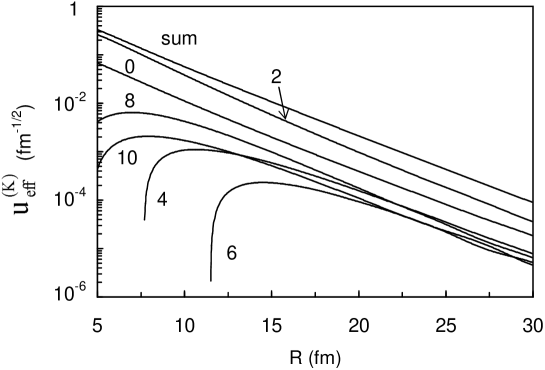
Figure 4: Same as in Fig. 3 in logarithmic scale.

The curves in Figs. 3 and 4 indicate that the product $u_{E}(R)u_{\rm eff}^{(K)}(R)$ for $K=0$ changes sign several times. The integral $I_{E}^{(0)}(R)$ is first positive, starts decreasing at the first zero of $u_{E}$, changes sign near 2 fm and increases again at the second zero of $u_{E}$. The combined effect of both zeros results in a cancellation between the internal and external parts of the corresponding limit $I_{E}^{(0)}(+\infty)$. These zeros at short distances are due to the existence of two bound states in the potential (one physical and one forbidden). The numbers and locations of zeros are typical of the ⁶He $\beta$ decay so that the cancellation should not occur for the decay of other halo nuclei. It would not occur so strongly with a single zero.

For $K=2$, the combined effects of the zero of $u_{\rm eff}^{(2)}$ and of the first zero of $u_{E}$ is just a small plateau near 2 fm in Fig. 2. The second zero of $u_{E}$ gives a minimum near 5 fm. The resulting $I_{E}^{(2)}(+\infty)$ for the $K=2$ component also yields an important cancellation, but not as strong as in the $K=0$ case.

The effective functions for $K=4$ and 6 are very small in the region where $u_{E}$ keeps a constant sign and lead to negligible contributions. Let us recall here that the convergence of low-$K$ components is not reached if $K_{\max}$ is not large enough DDB03 .

A new situation appears for the $K=8$ component. The effective wave function is much smaller than $K=0$ or 2 but the cancellation is minimal since it does not change sign. Hence it gives the second largest $I_{E}^{(K)}$ at infinity. The same mechanism applies for the smaller $K\geq 10$ components. The $K=10$ integral still contributes significantly to the total sum.

In Fig. 5, the integrals $I_{E}(R)=\sum_{K}I_{E}^{(K)}(R)$ calculated at the energy $E=1$ MeV are represented for the different potentials. The repulsive potential $V_{r}$ displays a strongly different behavior from the other potentials. At this energy, $V_{a}$ and $V_{f2}$ give almost the same result. This is due to the fact that, because of their similar phase shifts, their node near 5 fm in the scattering wave $u_{E}$ is at nearly the same location. The comparison with $V_{f1}$, where this node is about 1 fm farther away and leads therefore to weaker cancellation effects, shows the major role played by this node.

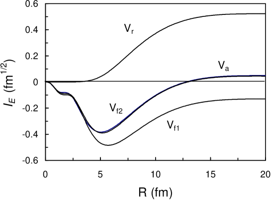
Figure 5: Integrals $I_{E}(R)=\sum_{K}I_{E}^{(K)}(R)$ at $E=1$ MeV calculated with $K_{\rm max}=24$ and $R_{\rm max}=30$ fm for different $\alpha+d$ potentials.

The $K=2$ and $K=8$ components of the three-body hyperspherical wave function of the ⁶He nucleus give dominant contributions to the integral $I_{E}(R)$ at large values of $R$ and thus to the Gamow-Teller reduced transition probability $B_{\rm GT}(E)$. This finding contradicts the assumption in Ref. zhu93 , that the $K=0$ and 2 dominant contributions to the energy are sufficient to study this $\beta$ decay mode.

III.3 Transition probability per time and energy units

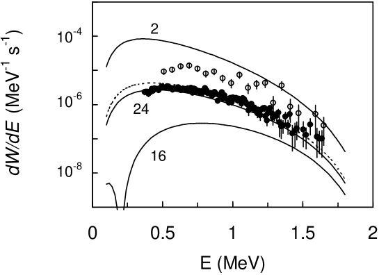
Figure 6: Transition probability per time and energy units $dW/dE$ of the ⁶He $\beta$ decay into the $\alpha+d$ continuum calculated with the $\alpha+d$ potential $V_{a}$ and $R_{\rm max}=30$ fm for several values of $K_{\rm max}$. Experimental data are from Refs. bor93 (open dots) and ABB02 (full dots). The dotted line corresponds to the $\alpha+N$ potential of Ref. KKN79 for the ⁶He wave function.

Before comparing transition probabilities with experiment, we discuss convergence aspects. To study the convergence with respect to the value of the maximal hypermomentum $K_{\rm max}$, we display in Fig. 6 the transition probabilities [Eq. (10)] calculated with potential $V_{a}$ for $K_{\rm max}=2$, 16, and 24. In each case the $\alpha+N$ interaction has been renormalized to reproduce the ⁶He binding energy. In a logarithmic scale, the results for $K_{\rm max}=22$ are essentially identical to those for $K_{\rm max}=24$. From Fig. 6, we can see that using large $K_{\rm max}$ values is crucial to obtain a good accuracy. This is analyzed in more detail below.

Additionally, the convergence is faster for the repulsive potential $V_{r}$ and for the folding potentials $V_{f1}$ and $V_{f2}$. In the case of $V_{r}$, the transition probabilities for $K_{\rm max}=16$ and $K_{\rm max}=24$ show almost the same features but have a larger value than for $V_{a}$. However, even in this case, the choice $K_{\rm max}=2$ in Ref. zhu93 is not realistic.

A calculation with $K_{\rm max}=24$ performed with the original wave function of Ref. DDB03 , i.e. with the $\alpha+n$ potential of Kanada et al KKN79 , and the $\alpha+d$ potential $V_{a}$ is displayed as a dotted line. The results are somewhat larger and in less good agreement with experiment at low energies but they nicely reproduce both the shape and order of magnitude of the data. This indicates that the present model is not much sensitive to details of the model describing the ⁶He wave function and confirms that convergence and an appropriate $\alpha+d$ potential are the crucial elements.

Table 1: Components $I_{E}^{(K)}(\infty)$ as a function of $K$ and $K_{\rm max}$ at $E=1$ MeV

$K$	$K_{\rm max}=2$	$K_{\rm max}=16$	$K_{\rm max}=18$	$K_{\rm max}=20$	$K_{\rm max}=22$	$K_{\rm max}=24$
$0$	$3.67\times 10^{-2}$	$2.84\times 10^{-3}$	$4.02\times 10^{-3}$	$5.21\times 10^{-3}$	$5.43\times 10^{-3}$	$5.74\times 10^{-3}$
$2$	$1.49\times 10^{-1}$	$-2.58\times 10^{-2}$	$-2.09\times 10^{-2}$	$-1.34\times 10^{-2}$	$-1.17\times 10^{-2}$	$-9.45\times 10^{-3}$
$4$		$4.99\times 10^{-3}$	$5.27\times 10^{-3}$	$4.75\times 10^{-3}$	$4.90\times 10^{-3}$	$4.78\times 10^{-3}$
$6$		$1.14\times 10^{-3}$	$1.13\times 10^{-3}$	$1.56\times 10^{-4}$	$5.12\times 10^{-5}$	$-3.06\times 10^{-4}$
$8$		$2.58\times 10^{-2}$	$2.66\times 10^{-2}$	$2.79\times 10^{-2}$	$2.84\times 10^{-2}$	$2.90\times 10^{-2}$
$10$		$8.64\times 10^{-3}$	$8.90\times 10^{-3}$	$9.37\times 10^{-3}$	$9.55\times 10^{-3}$	$9.78\times 10^{-3}$
$12$		$4.32\times 10^{-4}$	$4.15\times 10^{-4}$	$7.32\times 10^{-5}$	$8.38\times 10^{-6}$	$-1.50\times 10^{-4}$
$14$		$2.03\times 10^{-3}$	$2.14\times 10^{-3}$	$2.21\times 10^{-3}$	$2.26\times 10^{-3}$	$2.30\times 10^{-3}$
$16$		$2.01\times 10^{-3}$	$2.11\times 10^{-3}$	$2.33\times 10^{-3}$	$2.42\times 10^{-3}$	$2.53\times 10^{-3}$
$18$			$4.82\times 10^{-4}$	$4.70\times 10^{-4}$	$4.71\times 10^{-4}$	$4.62\times 10^{-4}$
$20$				$1.49\times 10^{-4}$	$1.45\times 10^{-4}$	$1.22\times 10^{-4}$
$22$					$3.26\times 10^{-4}$	$3.49\times 10^{-4}$
$24$						$1.59\times 10^{-4}$
sum	$1.86\times 10^{-1}$	$2.21\times 10^{-2}$	$3.01\times 10^{-2}$	$3.92\times 10^{-2}$	$4.23\times 10^{-2}$	$4.53\times 10^{-2}$

The low value of $dW/dE$ results from different cancellation effects which themselves are sensitive to the convergence of the different components of the three-body wave function. The final order of magnitude implies an accurate treatment of the convergence of the wave function and in particular of its halo part. In order to illustrate this mechanism, we display in Table 1 the numerical values of the components $I_{E}^{(K)}(\infty)$ of the Gamow-Teller integral for different values of the parameter $K_{\rm max}$ at 1 MeV. Let us start with $K_{\rm max}\geq 16$. For each value of $K_{\rm max}$, one observes that the dominant components are indeed $K=2$ and $K=8$. Components beyond $K=16$ become rather small. However, when $K_{\rm max}$ is increased, all components $I_{E}^{(K)}(\infty)$ of the matrix element are modified. As emphasized in Ref. DDB03 , increasing $K_{\rm max}$ in the three-body model does not only mean adding components but, even more, improving the convergence of lower $K$ components. This is illustrated when following a row in Table 1. The value of each component slowly converges when $K_{\rm max}$ is increased. If the experimental data were much more accurate, higher values of $K_{\rm max}$ should probably be considered.

The dominant $K=2$ and $K=8$ components have opposite signs. This effect adds another level of cancellation in the matrix element. It increases the role of the other components and especially the collective role of high-$K$ components. Finally a comparison with the first column shows why a calculation restricted to $K_{\rm max}=2$ has little meaning: the $K=2$ component is too large, has a wrong sign, and is not counterbalanced by other components.

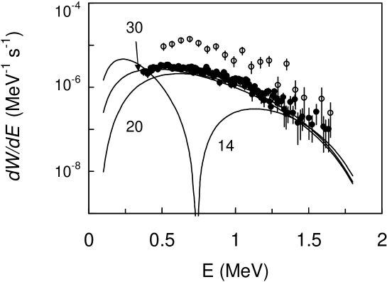
Figure 7: Transition probability per time and energy units $dW/dE$ of the ⁶He $\beta$ decay into the $\alpha+d$ continuum calculated with the $\alpha+d$ potential $V_{a}$ and $K_{\rm max}=24$ for several values of $R_{\rm max}$. Experimental data are from Refs. bor93 (open dots) and ABB02 (full dots).

In Fig. 7, the transition probability $dW/dE$ obtained with potential $V_{a}$ for a fixed $K_{\rm max}=24$ is presented for different values of $R_{\rm max}$, i.e., 14 fm, 20 fm, and 30 fm. Calculations for $R_{\rm max}=35$ fm show that convergent results are obtained at $R_{\rm max}\approx 30$ fm. Taking properly account of the halo extension is very important in a correct treatment of the very small transition probability $dW/dE$ of the ⁶He $\beta$ decay into $\alpha+d$.

In Fig. 8, we display the transition probability for different potentials, calculated with $K_{\rm max}=24$ and $R_{\rm max}=30$ fm. The best description of the experimental data of Ref. ABB02 is obtained with the attractive potential $V_{a}$. The worst results correspond to the repulsive potential $V_{r}$, which has no bound state and for which the description of the $s$-wave phase shift at low energies is poor. With potential $V_{r}$, the location of the nodes in the scattering wave does not lead to a cancellation (see Fig. 5). The folding potentials $V_{f1}$ and $V_{f2}$ have intermediate behaviors. Potential $V_{f1}$ overestimates the recent data while potential $V_{f2}$ provides a better order of magnitude but its energy dependence disagrees with the experimental one.

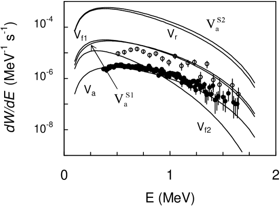
Figure 8: Transition probability per time and energy units $dW/dE$ of the ⁶He $\beta$ decay into the $\alpha+d$ continuum calculated with different $\alpha+d$ potentials for $K_{\rm max}=24$ and $R_{\rm max}=30$ fm. Experimental data are from Refs. bor93 (open dots) and ABB02 (full dots).

We have also performed a calculation with the original wave function of Ref. DDB03 and with a folding potential based on the $\alpha+n$ potential of Kanada et al KKN79 of $V_{f2}$ type, i.e. multiplied by 1.30 in order to fairly reproduce the phase shift. The results are indistinguishable from the curve labeled $V_{f2}$ at the scale of the figure. The shape of this curve is thus mostly due to the node locations of the $\alpha+d$ wave function.

The success of the deep Gaussian potential could be attributed to the fact that it simultaneously reproduces both the ⁶Li ground state binding energy and the $s$-wave phase shift at low energies. However the discussion of Figs. 2-4 indicates that an important ingredient is the existence of two nodes in $u_{\rm eff}$. In order to test this assumption, we remove the non-physical ground state of $V_{a}$ by using a pair of supersymmetric transformations Ba-87 . The resulting phase-equivalent potential $V_{a}^{S1}$ has exactly the same ⁶Li ground-state energy and the same $s$-wave phase shift as $V_{a}$ but its scattering wave functions have one node less at small distances. The resulting $dW/dE$ is about one order of magnitude larger and resembles the one obtained with the folding potential $V_{f1}$ (see Fig. 8). Notice however that $V_{f1}$ has two bound states but does not well reproduce the phase shifts. A second phase-equivalent potential $V_{a}^{S2}$ is obtained by removing the ⁶Li ground state from $V_{a}^{S1}$ with another pair of transformations. This repulsive potential has still exactly the same phase shifts as $V_{a}$ but no bound state. Its scattering wave functions have no node near the origin. As expected, the corresponding transition probability $dW/dE$ is now very close to the one obtained with potential $V_{r}$. The comparison emphasizes the crucial role played by the forbidden bound state, in addition to the physical ⁶Li ground state, for reproducing the order of magnitude of the experimental data.

The total transition probabilities for different potentials are given in the first row of Table 2. The second row contains results corresponding to the experimental cutoff ABB02 . The values in the last columns are derived from experimental branching ratios and from the ⁶He half life ABB02 . As expected from the previous discussion, the result obtained with the Gaussian potential $V_{a}$ falls within the experimental error bars of Ref. ABB02 . The other results are too large, especially with the repulsive potential.

Table 2: Total transition probability per second $W$ (in $10^{-6}$ s^-1) for the $\beta$ decay of ⁶He into $\alpha+d$.

	$V_{a}$	$V_{f1}$	$V_{f2}$	$V_{r}$	Exp. bor93	Exp. ABB02
$E>0$ MeV	$1.95$	$25.1$	$5.80$	$340$		$2.2\pm 1.1$
$E>0.37$ MeV	$1.54$	$18.2$	$3.32$	$246$	$7.6\pm 0.6$	$1.5\pm 0.8$

IV A comment on $R$-matrix fits

The $R$-matrix method has been extended by Barker bar94 to the $\beta$ delayed deuteron emission. It has been applied to analyze recent experimental results ABB02 . Like in other models, it is crucial in the $R$-matrix method to take care of the large extension of the halo. Without entering into details which are explained in Refs. bar94 ; ABB02 , this is achieved by introducing external corrections proportional to the integral

$$\mathcal{I}_{E}(a)=\int_{a}^{\infty}\frac{u_{i}(R)}{u_{i}(a)}u_{E}(R)dR,$$ (20)

where $a$ is the $R$-matrix channel radius and $u_{E}$ is replaced by its asymptotic expression (7). The factor $u_{i}(a)$ eliminates the problem of normalizing the approximation for the initial wave function $u_{i}(R)$. In Ref. bar94 , the notation $E_{i}(R)$ is used for $u_{i}(R)/u_{i}(a)$.

In the model of Ref. bar94 , the asymptotic form of the two-body $\alpha+$dineutron system is employed for $u_{i}$,

$$u_{i}^{\alpha+2n}(R)=\exp[-(2\mu_{(12)3}m_{N}|E_{B}|/\hbar^{2})^{1/2}R],$$ (21)

where $E_{B}=-0.975$ MeV. However, three-body asymptotics are rather different from this expression. In Eq. (15), this role is played by the effective radial wave function $u_{\rm eff}$ defined by Eq. (19). In order to avoid the knowledge of three-body wave functions, we suggest here an expression,

$$u_{i}^{\alpha+n+n}(R)=R\int_{0}^{\infty}\rho^{-5/2}\exp[-(2m_{N}|E_{B}|/\hbar^{2})^{1/2}\rho]ru_{d}(r)dr,$$ (22)

which is the projection of three-body asymptotics Me-74 ; DDB03 on the deuteron wave function. For a pointlike deuteron described with $u_{d}(r)\propto r^{-1}\delta(r)$, this function becomes

$$u_{i}^{\alpha+2n,{\rm cor.}}(R)=R^{-3/2}\exp[-(2\mu_{(12)3}m_{N}|E_{B}|/\hbar^{2})^{1/2}R].$$ (23)

It differs from Eq. (21) by the power factor $R^{-3/2}$. This simple expression also deserves being evaluated.

In Table 3, we present the integral (20) calculated with $u_{i}^{\alpha+2n}$, $u_{i}^{\alpha+n+n}$, $u_{i}^{\alpha+2n,{\rm cor.}}$, and $u_{\rm eff}$ at two typical energies for different values of the channel radius $a$.

Table 3: External integrals [Eq. (20)] in $R$-matrix fits: $\mathcal{I}_{E}^{\alpha+2n}$, $\mathcal{I}_{E}^{\alpha+2n,{\rm cor.}}$, $\mathcal{I}_{E}^{\alpha+n+n}$, and $\mathcal{I}_{E}^{\rm eff}$ are calculated with $u_{i}^{\alpha+2n}$ [Eq. (21)], $u_{i}^{\alpha+2n,{\rm cor.}}$ [Eq. (23)], $u_{i}^{\alpha+n+n}$ [Eq. (22)], and $u_{\rm eff}$ [Eq. (19)], respectively, for different values of the channel radius $a$ (in fm) and the relative energy $E$ (in MeV).

$E$	$a$	$\mathcal{I}_{E}^{\alpha+2n}$	$\mathcal{I}_{E}^{\alpha+2n,{\rm cor.}}$	$\mathcal{I}_{E}^{\alpha+n+n}$	$\mathcal{I}_{E}^{\rm eff}$
0.5	4.0	1.162	0.224	0.470	0.598
	4.5	1.391	0.384	0.651	0.751
	5.0	1.616	0.552	0.834	0.913
	5.5	1.834	0.726	1.018	1.082
	6.0	2.046	0.903	1.201	1.432
1.0	4.0	1.464	0.367	0.698	0.882
	4.5	1.754	0.601	0.952	1.091
	5.0	2.024	0.839	1.200	1.307
	5.5	2.172	1.075	1.437	1.522
	6.0	2.496	1.303	1.660	1.732

One observes that the results obtained with the two-body asymptotic expression (21) are rather far from the realistic values obtained with $u_{\rm eff}$, even for $a=6$ fm. A much better approximation is given by the three-body asymptotic expression (22), especially at higher relative energies. The corrected two-body approximation is smaller than the three-body approximation and not really close to the reference results.

In $R$-matrix theory however, because parameters are fitted, the absolute normalization of the integrals displayed in Table 3 is not important. It can be absorbed in a renormalization of the constants. The crucial property is their energy dependence. The four types of external integrals are shown in Fig. 9 as a function of energy for the typical value $a=5$ fm. One observes that $\mathcal{I}_{E}^{\alpha+2n,{\rm cor.}}$, $\mathcal{I}_{E}^{\alpha+n+n}$, and $\mathcal{I}_{E}^{\rm eff}$ have very similar energy dependences. On the contrary, $\mathcal{I}_{E}^{\alpha+2n}$ displays a different shape. Hence, using this approximation in $R$-matrix fits may significantly distort the energy shape of the $\beta$ delayed deuteron spectrum. The $\alpha+n+n$ approximation offers a very good approximation of the model results. Nevertheless, the corrected two-body expression provides the simplest significant improvement for $R$-matrix calculations.

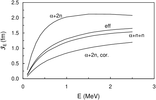
Figure 9: External integrals $\mathcal{I}_{E}^{\alpha+2n}$, $\mathcal{I}_{E}^{\alpha+2n,{\rm cor.}}$, $\mathcal{I}_{E}^{\alpha+n+n}$, and $\mathcal{I}_{E}^{\rm eff}$ as a function of the relative energy $E$ for $a=5$ fm.

V Conclusions

In the present work, we studied the $\beta$-decay process of the ⁶He halo nucleus into the $\alpha+d$ continuum in the framework of a three-body model. Three-body hyperspherical bound-state wave functions on a Lagrange mesh and two-body $\alpha+d$ scattering wave functions have been used. For the calculation of the $\beta$-decay transition probabilities per time and energy units, several $\alpha+d$ potentials were tested: an attractive Gaussian potential dub94 with a deep forbidden bound state, folding potentials derived from the $\alpha+N$ $p$-wave potential of Ref. vor95 , and a repulsive potential zhu93 .

We confirm that the low experimental values result from a strong cancellation in the Gamow-Teller matrix element describing the transition to the continuum BSD94 . This cancellation occurs between the internal and halo parts of the matrix element and is thus very sensitive to the halo description. Reaching convergence is not easy: the two-body and three-body wave functions must extend up to about 30 fm. From the analysis of the theoretical results, we have found that converged results require large values of the maximal hypermomentum $K_{\rm max}$. The dominant contributions to the transition probability come from the $K=2$, $K=8$, and $K=10$ components of the three-body hyperspherical wave function. The $K=0$ contribution is small due to an almost perfect cancellation of its internal and external parts in the Gamow-Teller matrix element. The $K=2$ and $K=8$ components have opposite signs which enhances the importance of other, and especially high-$K$, components.

The experimental transition probabilities per time and energy units of Ref. ABB02 are well described with the deep Gaussian potential of Ref. dub94 which fairly reproduces the ⁶Li binding energy and the $\alpha+d$ $s$-wave phase shifts. The quality of the agreement arises from the node structure of the initial and final wave functions in the internal part. With the help of phase-equivalent potentials derived with supersymmetric transformations, we have shown that the role of the forbidden state is also essential. We realize that the efficiency of the deep potential may be somewhat fortuitous since the nodes of the scattering wave function have to be at very precise locations. The fact that the data can be reproduced does not mean that the present model or the simple Gaussian potential are perfect. However the reasonable agreement with the data obtained with the same $\alpha+d$ potential but another ⁶He wave function indicates that the present model interpretation should be trustable. Most importantly the existence of a good agreement with experiment points toward the ingredients that are crucial in the interpretation of the $\beta$ delayed deuteron decay of ⁶He. One can expect a completely different behavior for this $\beta$-decay mode in the case of ¹¹Li. Indeed the ⁶He-case cancellations require precise numbers of nodes and precise locations of these nodes and it is very unlikely that this could occur so perfectly in another case.

Our results allow testing the validity of external corrections necessary in the $R$-matrix method bar94 . We have shown that, in order to reduce a systematic bias in the integrals over the external region, the two-body asymptotics can usefully be replaced by three-body asymptotics or, more simply, be corrected by a factor $R^{-3/2}$.

Further progress on this $\beta$-decay mode must come from consistent fully microscopic descriptions of the bound and scattering states. The results obtained with a microscopic cluster model cso94 still agree qualitatively with the most recent data ABB02 but overestimate them by about a factor of two. Progress may be expected from the possibility of calculating ⁶He wave functions ab initio PWC04 from realistic two- and three-body forces. However the present study shows that a successfull description of the $\beta$ delayed deuteron emission will require very accurate bound-state wave functions up to distances as large as 30 fm and a development of consistent scattering wave functions. The accidental cancellation occurring in this process will make a fully ab initio description particularly difficult.

References

- (1) I. Tanihata, J. Phys. G 22, 157 (1996).
- (2) P.G. Hansen and B. Jonson, Europhys. Lett. 4, 409 (1987).
- (3) M.V. Zhukov, D.V. Fedorov, B.V. Danilin, J.S. Vaagen, and J.M. Bang, Nucl. Phys. A529, 53 (1991).
- (4) K. Riisager, M.J.G. Borge, H. Gabelmann, P.G. Hansen, L. Johannsen, B. Jonson, W. Kurcewicz, G. Nyman, A. Richter, O. Tengblad, K. Wilhelmsen, and ISOLDE Collaboration, Phys. Lett. B235, 30 (1990).
- (5) M.J.G. Borge, L. Johannsen, B. Jonson, T. Nilsson, G. Nyman, K. Riisager, O. Tengblad, and K. Wilhelmsen Rolander, Nucl. Phys. A560, 664 (1993).
- (6) D. Anthony, L. Buchmann, P. Bergbusch, J.M. D’Auria, M. Dombsky, U. Giesen, K.P. Jackson, J.D. King, J. Powell, and F.C. Barker, Phys. Rev. C 65, 034310 (2002).
- (7) P. Descouvemont and C. Leclercq-Willain, J. Phys. G 18, L99 (1992).
- (8) M.V. Zhukov, B.V. Danilin, L.V. Grigorenko, and N.B. Shul’gina, Phys. Rev. C 47, 2937 (1993).
- (9) D. Baye, Y. Suzuki, and P. Descouvemont, Prog. Theor. Phys. 91, 271 (1994).
- (10) K. Varga, Y. Suzuki, and Y. Ohbayasi, Phys. Rev. C 50, 189 (1994).
- (11) F.C. Barker, Phys. Lett. B322, 17 (1994).
- (12) A. Csótó and D. Baye, Phys. Rev. C 49, 818 (1994).
- (13) P. Descouvemont, C. Daniel, and D. Baye, Phys. Rev. C 67, 044309 (2003).
- (14) D. Baye and P.-H. Heenen, J. Phys. A 19, 2041 (1986).
- (15) S.B. Dubovichenko and A.V. Dzhazairov-Kakhramanov, Phys. Atom. Nucl. 57, 733 (1994).
- (16) V.T. Voronchev, V.I. Kukulin, V.N. Pomerantsev, and G.G. Ryzhikh, Few-Body Syst. 18, 191 (1995).
- (17) D. Baye and P. Descouvemont, Nucl. Phys. A481, 445 (1988).
- (18) D.H. Wilkinson, Nucl. Phys. A377, 474 (1982).
- (19) D. Dubbers, W. Mampe, and J. Dohner, Europhys. Lett. 11, 195 (1990).
- (20) M.C. Abramowitz and I.A. Stegun, Handbook of Mathematical Functions (Dover, New York, 1970).
- (21) D.R. Thompson, M. LeMere, and Y.C. Tang, Nucl. Phys. A286, 53 (1977).
- (22) H. Kanada, T. Kaneko, S. Nagata, and M. Nomoto, Prog. Theor. Phys. 61, 1327 (1979).
- (23) W. Grüebler, P.A. Schmelzbach, V. König, R. Risler, and D. Boerma, Nucl. Phys. A242, 265 (1975).
- (24) B. Jenny, W. Grüebler, V. König, P.A. Schmelzbach, and C. Schweizer, Nucl. Phys. A397, 61 (1983).
- (25) D. Baye, Phys. Rev. Lett. 58, 2738 (1987); J. Phys. A 20, 5529 (1987).
- (26) S.P. Merkur’ev, Yad. Fiz. 19, 447 (1974) [Sov. J. Nucl. Phys. 19, 222 (1974)].
- (27) S.C. Pieper, R.B. Wiringa, and J. Carlson, Phys. Rev. C 70, 054325 (2004).