Inhomogeneous freeze-out in relativistic heavy-ion collisions

Abstract

A QCD phase transition may reflect in a inhomogeneous decoupling surface of hadrons produced in relativistic heavy-ion collisions. We show that due to the non-linear dependence of the particle densities on the temperature and baryon-chemical potential such inhomogeneities should be visible even in the integrated, inclusive abundances. We analyze experimental data from Pb+Pb collisions at CERN-SPS and Au+Au collisions at BNL-RHIC to determine the amplitude of inhomogeneities.

I Introduction

Collisions of heavy nuclei at relativistic energies produce very hot and baryon-dense QCD matter HI . The entropy per net baryon in the central region increases monotonically with beam energy, i.e. the maximum temperature increases, while the baryon-chemical potential decreases. Hence, by varying the energy as well as the mass number of the nuclei etc., one can explore various regimes of the phase diagram of QCD. In particular, it is expected that at sufficiently high energies a transient state of deconfined matter with broken $Z(3)$ center symmetry and/or with (approximately) restored chiral symmetry is produced.

Lattice QCD simulations Fodor:2001pe indicate that a second-order critical point exists, which was predicted by effective chiral Lagrangians SRS ; present estimates locate it at $T\approx 160$ MeV, $\mu_{B}\approx 360$ MeV. This point, where the $\sigma$-field is massless, is commonly assumed to be the endpoint of a line of first-order phase transitions in the $(\mu_{B},T)$ plane.

There is an ongoing experimental effort to detect the line of first-order phase transitions at high baryon density, and its possible endpoint, in heavy-ion collisions. It is hoped that by varying the beam energy, for example, one can “switch” between the regimes of first-order phase transition and cross over, respectively. If the particles decouple shortly after the expansion trajectory crosses the line of first order transitions one may expect a rather inhomogeneous (energy-) density distribution on the freeze-out surface Bower:2001fq ; Paech:2003fe (similar, say, to the CMB photon decoupling surface observed by WMAP wmap ). On the other hand, if the low-temperature and high-temperature regimes are smoothly connected, pressure gradients tend to wash out density inhomogeneities. Similarly, in the absence of phase-transition induced non-equilibrium effects, the predicted initial-state density inhomogeneities iniflucs ; spherio should be strongly damped.

Here, we investigate the properties of an inhomogeneous fireball at (chemical) decoupling. Note that if the scale of these inhomogeneities is much smaller than the decoupling volume then they can not be resolved individually, nor will they give rise to large event-by-event fluctuations. Because of the nonlinear dependence of the hadron densities on $T$ and $\mu_{B}$, they should nevertheless reflect in the average abundances. Our goal is to check whether the experimental data shows any signs of inhomogeneities on the freeze-out surface.

Our basic assumption is that as the fireball expands and cools, at some stage the abundances of hadrons “freeze”, keeping memory of the last instant of chemical equilibrium. This stage is refered to as chemical freeze-out. By definition, only processes that conserve particle number for each species individually, or decays of unstable particles may occur later on.

The simplest model is to treat the gas of hadrons within the grand canonical ensemble, assuming a homogeneous decoupling volume. The abundances are then determined by two parameters, the temperature $T$ and the baryonic chemical potential $\mu_{B}$; the chemical potential for strangeness is fixed by the condition for overall strangeness neutrality, and other conserved charges shall be neglected. Fits of hadronic ratios were performed extensively Pbm05 ; thermo within this model, sometimes also including a strangeness ($\gamma_{s}$) or light quark ($\gamma_{q}$) supression factor thermo_gammas ; Becc05 or interactions with the chiral condensate thermo_int .

The purpose of the present paper is to analyze the experimental data on relative abundances of hadrons with respect to the presence of inhomogeneities on the decoupling surface. To that end, we propose a very simple and rather schematic extension of the common grand canonical freeze-out model, i.e. a superposition of such ensembles with different temperatures and baryon-chemical potentials. Each ensemble is supposed to describe the local freeze-out on the scale of the correlation length $\sim 1/T\sim 1-2$ fm. Even if freeze-out occurs near the critical point, the correlation length of the chiral condensate is bound from above by finite size and finite time effects, effectively resulting in similar numbers corr_length . On the other hand, for small chemical potential, far from the region where the $\sigma$-field is critical, the relevant scale might be set by the correlation length for Polyakov loops, which is of comparable magnitude loop_corlength . Classical nucleation theory for strong first-order phase transitions predicts even larger “bubbles” nucleation but is unlikely to apply to small, rapidly expanding systems encountered in heavy-ion collisions Paech:2003fe ; Scavenius:2000bb . Another (classical) model for the formation of small droplets in rapidly expanding QCD matter has been introduced in Mishustin:1998eq .

The entire decoupling surface contains many such “domains”, even if a cut on mid-rapidity is performed. We therefore expect that the distributions of temperature and chemical potential are approximately Gaussian. Besides simplicity, another goal of the present analysis is to avoid reference to a particular dynamical model for the formation or for the distribution of density perturbations. In fact, we presently aim merely at checking whether any statistically significant signal for the presence of inhomogeneities is found in the data. If so, more sophisticated dynamical models could be employed in the future to understand the evolution of inhomogeneities from their possible formation in a phase transition until decoupling.

Rate equations for nuclear fusion and dissociation processes (and neutron diffusion) have been used for inhomogeneous big bang nucleosynthesis in the early universe iBBN . Similarly, hadronic cascade models could be used for heavy-ion reactions HydroCascade . This would remove reference to the grand-canonical ensemble and to a thin decoupling surface in space-time. In fact, hadronic binary rescattering models do predict a rather thick freeze-out layer HydroCascade ; sorge , where matter expands non-ideally. On the other hand, the steep drop of multi-particle collision rates with temperature should narrow the freeze-out again BSW . In either case, we do not expect a strong energy dependence of the width of freeze-out (see also ceres ).

At chemical freeze-out, matter is in a state of expansion. However, such flow effects do not affect the relative abundances of the particles (in full phase space) if their densities are homogeneous throughout the decoupling volume. The total number of particles of species $i$, integrated over a solid angle of $4\pi$, is given by an integral of the current $N_{i}^{\mu}=\rho_{i}\,u^{\mu}$, with $u^{\mu}$ the four-velocity of the expanding fluid, over a given freeze-out hypersurface $\sigma^{\mu}=(t^{\rm fo},\vec{x}^{\rm\,fo})$:

$$N_{i}=\int d\sigma_{\mu}N_{i}^{\mu}=\rho_{i}(T^{\rm fo},\mu_{B}^{\rm fo})\int u^{\mu}d\sigma_{\mu}~{}.$$ (1)

The second factor on the r.h.s. is nothing but the three-volume $V_{3}$ of the decoupling hypersurface as seen by the observer. This volume is common to all species and drops out of multiplicity ratios: $N_{i}/N_{j}=\rho_{i}^{\rm fo}/\rho_{j}^{\rm fo}$. It is clear that the argument holds even when cuts in momentum space are performed, provided that the differential distributions of all particles do not depend on that particular momentum-space variable (for example, rapidity cuts for boostinvariant expansion CleyRed99 ).

When the intensive variables $T$ and $\mu_{B}$ vary, then the integration measure $(\int u\cdot d\sigma)/V_{3}$ will, in general, depend on the assumed distribution and amplitude of inhomogeneities, as well as on the hydrodynamic flow profile etc. Nevertheless, it is still the same for all particle species and so can be written in the form

$${1\over V_{3}}\int u\cdot d\sigma\longrightarrow\int dTd\mu_{B}\,P(T,\mu_{B})~{},$$ (2)

with $P(T,\mu_{B})$ some distribution for $T$ and $\mu_{B}$. For simplicity, and for lack of an obvious motivation for assuming otherwise, we shall take $P(T,\mu_{B})$ to factorize into a distribution for $T$, times one for $\mu_{B}$. These distributions could, in principle, be obtained from the real-time evolution of the phase transition Bower:2001fq ; Paech:2003fe .

II The model

With these qualifications aside, we now proceed to introduce our model and to analyze the available data from heavy-ion collisions at high energies. The hadron abundances are determined by four parameters: the arithmetic means of the temperatures and chemical potentials of all domains, $\overline{T}$ and $\overline{\mu}_{B}$, and the widths of their Gaussian distributions, $\delta T$ and $\delta\mu_{B}$. Then, the average density of species $i$ is computed as

$$\overline{\rho}_{i}\;(\overline{T},\overline{\mu}_{B},\delta T,\delta\mu_{B})=$$ (3)

$$\int\limits_{0}^{\infty}dT\;P(T;\overline{T},\delta T)\int\limits_{-\infty}^{\infty}d\mu_{B}\;P(\mu_{B};\overline{\mu}_{B},\delta\mu_{B})~{}\rho_{i}(T,\mu_{B})~{},$$

with $\rho_{i}(T,\mu_{B})$ the actual “local” density of species $i$, and with $P(x;\overline{x},\delta x)\sim\exp[-{\left(x-\overline{x}\right)^{2}}/{2\,\delta x^{2}}]$ the distribution of temperatures and chemical potentials within the decoupling three-volume (the proportionality constants normalize the distributions over the intervals where they are defined). In the limit $\delta T$, $\delta\mu_{B}\to 0$ the Gaussian distributions are replaced by $\delta$-functions and the conventional homogeneous freeze-out scenario is recovered: $\overline{\rho}_{i}\;(\overline{T},\overline{\mu}_{B},0,0)=\rho_{i}(\overline{T},\overline{\mu}_{B})$. In other words, in that limit the average densities are uniquely determined by the first moments of $T$ and $\mu_{B}$.

For the present analysis we compute the densities $\rho_{i}(T,\mu_{B})$ in the ideal gas approximation, supplemented by an “excluded volume” correction:

$$\rho_{i}(T,\mu_{B})=\frac{\rho_{i}^{\rm id-gas}(T,\mu_{B})}{1+v_{i}\sum_{j}\rho_{j}^{\rm id-gas}}~{}.$$ (4)

This schematic correction models repulsive interactions among the hadrons at high densities. $v_{i}$ denotes the volume occupied by a hadron of species $i$; we employ $v=\frac{4}{3}\pi{R_{0}}^{3}$ with $R_{0}=0.3$ fm for all species ExclVol . Therefore, for the homogeneous model the denominator in (4) drops out of multiplicity ratios. This is not the case for an inhomogeneous decoupling surface, where the distributions of various species differ.

The densities of strange particles depend also on the strangeness-chemical potential $\mu_{S}$, which we determine by imposing local strangeness neutrality. Strictly speaking, this condition is not mandatory, of course. The effect of independent fluctuations of $\mu_{S}$ should be looked at in the future, in particular for collisions at low and intermediate energies ($\surd s_{NN}\mbox{\raisebox{-2.58334pt}{$\stackrel{{\scriptstyle<}}{{\sim}}$}}\>15$ GeV). This may help to reproduce the $\overline{\Lambda}$ to $\overline{p}$ ratio, which was found to be larger than one inh_mus and the $K^{+}/\pi^{+}$ enhancement around $E_{\rm{Lab}}/A=30$ GeV Na49_data . For all fits over the full solid angle, we fixed the isospin chemical potential by equating the total charge in the initial and final states; for the mid-rapidity fits at high energies, we fixed $\mu_{I}=0$.

To illustrate the effect of inhomogeneities on the distributions of various hadrons within the decoupling volume we introduce

$$D_{i}(T;\overline{T},\overline{\mu}_{B},\delta T,\delta\mu_{B})=P(T;\overline{T},\delta T)$$

$$\hskip 28.45274pt\times\frac{\int\limits_{-\infty}^{\infty}d\mu_{B}\;P(\mu_{B};\overline{\mu}_{B},\delta\mu_{B})~{}\rho_{i}(T,\mu_{B})~{}}{\overline{\rho}_{i}\;(\overline{T},\overline{\mu}_{B},\delta T,\delta\mu_{B})}~{},$$ (5)

$$D_{i}(\mu_{B};\overline{T},\overline{\mu}_{B},\delta T,\delta\mu_{B})=P(\mu_{B};\overline{\mu}_{B},\delta\mu_{B})$$

$$\hskip 28.45274pt\times\frac{\int\limits_{0}^{\infty}dT\;P(T;\overline{T},\delta T)~{}\rho_{i}(T,\mu_{B})~{}}{\overline{\rho}_{i}\;(\overline{T},\overline{\mu}_{B},\delta T,\delta\mu_{B})}~{}.$$ (6)

$D_{i}(T)$, for example, is the probability that a particle of type $i$ was emitted from a domain of temperature $T$. The main contribution to the integrals in (3) is not from $\overline{T}$ and $\overline{\mu}_{B}$ since hot spots shine brighter than “voids”. Rather, they are dominated by the stationary points of the distributions defined in eqs. (5,6) above. Hence, the average emission temperature $\langle T\rangle_{i}$ and baryon-chemical potential $\langle\mu_{B}\rangle_{i}$ in general depend on the particle species $i$, unless $\delta T=\delta\mu_{B}=0$. They can be evaluated as

$$\langle T\rangle_{i} = \int\limits_{0}^{\infty}dT\;T\;D_{i}(T;\overline{T},\overline{\mu}_{B},\delta T,\delta\mu_{B})~{},$$

$$\langle\mu_{B}\rangle_{i} = \int\limits_{-\infty}^{\infty}d\mu_{B}\;\mu_{B}\;D_{i}(\mu_{B};\overline{T},\overline{\mu}_{B},\delta T,\delta\mu_{B})~{}.$$ (7)

Physically, this means that for non-zero widths of the temperature and chemical potential distributions the freeze-out volume is not perfectly “stirred”, in that the relative concentrations of the particles vary.

For some limiting cases one can estimate the effect analytically. Consider first massless particles without chemical potential ($\approx$ direct pions):

$$D(T;\overline{T},\delta T)\sim\exp\left(3\log\frac{T}{\overline{T}}-\frac{\left(T-\overline{T}\right)^{2}}{2\;\delta T^{2}}\right)~{}.$$ (8)

To leading order in $\delta T/\overline{T}$ the stationary point of the exponential is

$$\frac{T^{*}}{\overline{T}}=1+3\frac{\delta T^{2}}{\overline{T}^{2}}+\cdots$$ (9)

Hence, massless particles are not very sensitive to small fluctuations in temperature. They are typically emitted from regions with temperature $\approx\overline{T}$, up to quadratic corrections in ${\delta T}/{\overline{T}}$. In other words, the “particle emission distribution” $D(T)$ is shifted (and skewed) only slightly from the “temperature distribution” $P(T)$. This, of course, is simply due to the $\rho\sim T^{3}$ power-law form of the local density of massless particles. The convolution of a (narrow) Gaussian with a power-law does not lead to a large shift of the peak.

Next, we consider the more interesting case of massive particles with chemical potential equal to $\mu_{B}$ (for anti-baryons replace $\overline{\mu}_{B}\to-\overline{\mu}_{B}$ etc.). We assume that $\exp[(\mu_{B}-m)/T]\ll 1$ and $m/T\gg 1$ such that quantum statistical and relativistic corrections can be neglected, but allow that $x\equiv(m/\overline{T})(\delta T^{2}/\overline{T}^{2})={\cal O}(1)$. The integral over $\mu_{B}$ is then straightforward, leading to the particle distribution

$$D(T)\;\sim\;$$

$$\exp\left(\frac{3}{2}\log(T/\overline{T})+\frac{\mu_{B}-m}{T}+\frac{{\delta\mu_{B}}^{2}}{2{\overline{T}}^{2}}-\frac{\left(T-\overline{T}\right)^{2}}{2\;\delta T^{2}}\right)~{}.$$ (10)

Again, we look for the stationary point of the exponential. To leading order in the Gaussian width,

$$\frac{T^{*}}{\overline{T}} = 1+\frac{{\delta T}^{2}}{{\overline{T}}^{2}}\left(\frac{m}{\overline{T}}-\frac{\mu_{B}}{\overline{T}}+\frac{3}{2}\right)$$ (11)

$$= 1+\frac{{\delta T}^{2}}{{\overline{T}}^{2}}\left(\frac{m}{\overline{T}}+O(1)\right)\simeq 1+x~{}.$$

In the second step, we have used the fact that in the Boltzmann limit ${\mu_{B}}/{\overline{T}}$ is of order 1 (i.e., not parametrically large). Hence, for massive particles the distribution is shifted by a large amount $x={\cal O}(1)$. Their emission is dominated by the tails of the Gaussian distribution or, in physical terms, by rare “hot spots”.

To estimate the increase of the average density relative to the homogeneous case we plug the expression for $T^{*}$ into $D(T)$ from eq. (10), which gives

$$\frac{\overline{\rho}(\overline{T},\delta T,\overline{\mu}_{B},\delta\mu_{B})}{\rho(\overline{T},\overline{\mu}_{B})}=$$

$$\hskip 28.45274ptf\,\exp\left(\frac{1}{(1+x)^{2}}\,\frac{{\delta\mu_{B}}^{2}}{2\,{\overline{T}}^{2}}+\frac{x}{1+x}\,\frac{m-\overline{\mu}_{B}}{\overline{T}}\right)~{}.$$ (12)

The non-exponential prefactor $f$ arises due to the changing width of the integration measure when the temperature is inhomogeneous and can not be estimated by a saddle-point integration ($f=1$ for $\delta T=0$). Regardless, the main issue here is that this ratio increases exponentially with $(\delta\mu_{B}/\overline{T})^{2}$. Hence, we conclude that small fluctuations in the chemical potential are sufficient to raise the number of heavy particles significantly. Note that what matters is the magnitude of $\delta\mu_{B}$ relative to $\overline{T}$, not $\overline{\mu}_{B}$.

Similarly, temperature inhomogeneities also increase the density exponentially. That is, for $\delta T\rightarrow 0$, $x/(1+x)\approx x$. However, the growth saturates when $x\sim 1$. The enhancement factor from $x=0$ to $x\sim 1$ is very large, $\sim\surd\exp\left({(m-\overline{\mu}_{B})}/{\overline{T}}\right)$.

III Data analysis

To determine the four parameters of the model we minimize

$$\chi^{2}=\sum_{i}{\left(r_{i}^{exp}-r_{i}^{model}\right)^{2}}/{\sigma_{i}^{2}}$$ (13)

in the space of $\overline{T}$, $\overline{\mu}_{B}$, $\delta T$, and $\delta\mu_{B}$. That is, we obtain least-square estimates for the parameters, assuming that they are independent. In (13), $r_{i}^{exp}$ and $r_{i}^{model}$ denote the experimentally measured and the calculated particle ratios, respectively, and $\sigma_{i}^{2}$ is set by the uncertainty of the measurement. Wherever available, we sum systematic and statistical errors in quadrature.

The data used in our analysis are the particle multiplicities measured by the NA49 collaboration for central Pb+Pb collisions at beam energy $E_{\rm Lab}/A=20$, 30, 40, 80 and 158 GeV Na49_data , and those measured by STAR for central Au+Au collisions at BNL-RHIC, ref. RHIC130_data ($\surd{s_{NN}}=130$ GeV, compiled in RHIC_130_comp ) and ref. RHIC_data (200 GeV). At RHIC energies, we analyze the midrapidity data; at top SPS energy, both, midrapidity and $4\pi$ data. At all other energies, we restrict ourselves to the $4\pi$ solid angle data by NA49 in order to avoid biases arising from differing acceptance windows of various experiments. Furthermore, our checks showed that the fit results can depend somewhat on the actual selection of experimental ratios. Hence, where possible, we have opted for the least bias by choosing $r_{i}^{exp}=N^{exp}_{i}/N^{exp}_{\pi}$, i.e. the multiplicity of species $i$ relative to that of pions. This represents the maximal set of independent data points, as it is equivalent to fitting absolute multiplicities with an additional overall three-volume parameter, $N_{i}=V_{3}\rho_{i}$.

Specifically, at $E_{\rm Lab}/A=20$, 30, and 80 GeV the multiplicities of $\pi^{+}$, $\pi^{-}$, $K^{+}$, $K^{-}$, $B-\overline{B}$, $\Lambda$, $\overline{\Lambda}$, and $\phi$ are available. For the (in-)homogeneous model, this leaves five (three) degrees of freedom. At 40 GeV, we can add the $\Xi^{-}$ and $\Omega+\overline{\Omega}$. The data sets for top SPS energies include yet a few more species: $p$, $\overline{p}$ (only midrapidity), $K^{0}_{S}$ (only $4\pi$), $\overline{\Xi}^{+}$ and $\Omega$, $\overline{\Omega}$ seperately. For RHIC-130, we fitted to the $K^{+}/K^{-}$, $\overline{p}/p$, $\overline{\Lambda}/\Lambda$, $\Xi^{+}/\Xi^{-}$, $\overline{\Omega}/\Omega$, $K^{-}/\pi^{-}$, $K^{0}_{S}/\pi^{-}$, $\overline{p}/\pi^{-}$, $\Lambda/\pi^{-}$, $K_{0}^{\ast}/\pi^{-}$, $\phi/\pi^{-}$, $\Xi^{-}/\pi^{-}$ and $\Omega/\pi^{-}$ ratios. Finally, at RHIC-200 the $K^{+}/K^{-}$, $\overline{p}/p$, $\overline{\Omega}/\Omega$, $K^{-}/\pi^{-}$, $\overline{p}/\pi^{-}$, $\Lambda/\pi^{-}$, $\overline{\Lambda}/\pi^{-}$, $\Xi^{-}/\pi^{-}$, $\Xi^{+}/\pi^{-}$, $\Omega/\pi^{-}$, $\phi/K^{-}$ and $K_{0}^{\ast}/K^{-}$ ratios were used. The first three ratios are close to unity and essentially just set the chemical potentials to zero; they do not help to fix $\overline{T}$, $\delta T$ and $\delta\mu_{B}$.

Where appropriate, feeding from strong and electromagnetic decays has been included in $r^{model}_{i}$ by replacing ${\rho}_{i}\rightarrow{\rho}_{i}+B_{ij}\;{\rho}_{j}.$ The implicit sum over $j\neq i$ runs over all unstable hadron species, with $B_{ij}$ the branching ratio for the decay $j\to i$, which were taken from PDG . From all the resonances listed by the Particle Data Group PDG , mesons up to a mass of 1.5 GeV and baryons up to a mass of 2 GeV were included, respectively. The finite widths of the resonances were not taken into account, and unknown branching ratios were excluded from the feeding. These details are irrelevant for the qualitative behavior of $\delta T$ and $\delta\mu_{B}$ but do, of course, matter for quantitative results. For SPS energies, feeding from weak decays was included only for the ${\Xi}\to\Lambda$ and $\Omega\to\Lambda$ channels (and the corresponding decays of the anti-baryons) at $E_{\rm Lab}/A=20$ and 30 GeV. All other experimental yields were already corrected by NA49 for feed-down from weak decays Na49_data . At RHIC energies, feeding from weak decays has to be taken into account for a variety of particle species, c.f. RHIC130_data ; RHIC_data .

Technically, our fits use a four-dimensional lookup table for $\overline{\rho}_{i}$ with 1 MeV steps in $T$ and $\delta T$ and $10$ MeV steps in $\mu$ and $\delta\mu$ for the inhomogeneous fits, and 1 MeV steps for both $T$ and $\mu$ for the homogeneous fits. The finite grid of course limits our ability to determe the best fit. However, the effect was checked to be small, so that the accuracy should be sufficient to investigate the qualitative behavior of inhomogeneities, and whether they can improve the agreement with the experimental data significantly.

IV Results

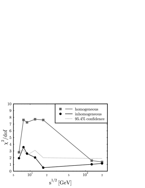
Figure 1: $\chi^{2}/dof$ versus $\surd{s_{NN}}$ for the homogeneous ($\delta T=\delta\mu=0$, squares) and the inhomogeneous fit ($\delta T$ and $\delta\mu$ free parameters, circles). The full and dashed lines are meant to guide the eye. Furthermore, the $\chi^{2}/dof$ corresponding to the $95.4\%$ confidence interval is shown by the dotted line.

Fig. 1 shows the minimal $\chi^{2}$ per degree of freedom (taken as the number of data points minus the number of parameters) for the homogeneous and the inhomogeneous approach, respectively. At $E_{\rm Lab}/A=20$ GeV and at RHIC energies, $\chi^{2}/dof$ is similar for both models. Thus, the inhomogeneous model does not provide a statistically significant improvement of the description of the measured particle ratios. Hence, the assumption of a nearly homogeneous decoupling surface can not be rejected for low SPS and RHIC energies.

On the other hand, for intermediate SPS energies, $E_{\rm Lab}/A\simeq 30-160$ GeV, $\chi^{2}/dof$ is considerably smaller for the inhomogeneous freeze-out surface than for the homogeneous case, which is far outside the 95.4% confidence interval spsfits . This indicates that the parameters of the inhomogeneous model are well determined and have reasonably small error bars. It is worth noting that, in general, the improvement is not driven by one single species; rather, the inhomogeneous model describes nearly all multiplicities better than a homogeneous decoupling surface Bormio . We also stress that our fits with $\delta T=\delta\mu_{B}=0$ reproduce results from the literature thermo ; thermo_gammas ; RHIC_data if the same input ratios are selected.

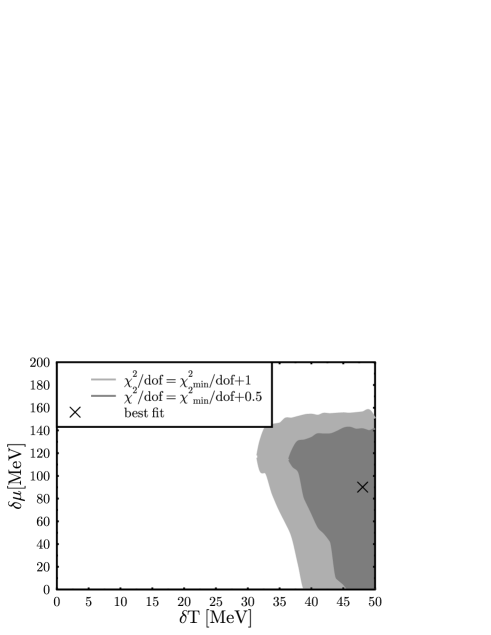
Figure 2: $\chi^{2}/dof$ contours in the $\delta T$, $\delta\mu_{B}$ plane for top SPS energy, $E_{\rm Lab}=158$ GeV. The other two parameters ($\bar{T}$, $\bar{\mu}_{B}$) are allowed to vary freely. The $\chi^{2}/dof$ minimum is indicated by the cross.

To illustrate the significance of inhomogeneities differently, we show contours of $\chi^{2}/dof$ in the plane of $\delta T$, $\delta\mu_{B}$ in figs. 2 and 3. Here, $\overline{T}$ and $\bar{\mu}_{B}$ were allowed to vary freely such as to minimize $\chi^{2}$ at each point. Fig. 2 shows that $\chi^{2}$ is relatively flat along the $\delta\mu_{B}$ direction, while $\delta T$ is determined more accurately and is clearly non-zero. In general we find that there is little correlation between $\delta T$ and $\delta\mu_{B}$ and that about the minimum, $\chi^{2}$ is rather flat in $\delta\mu_{B}$ direction.

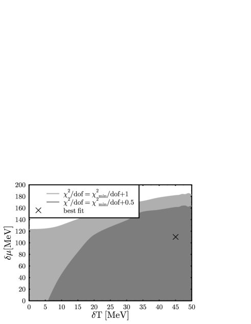
Figure 3: Same as fig. 2 for RHIC energy ($\surd{s_{NN}}=200$ GeV).

On the other hand, Fig. 3 shows that at RHIC energy, $\chi^{2}$ is very flat in both directions. With the present data points, a homogeneous freeze-out model appears to be a reasonable approximation at high energies. We have traced the origin of the very flat $\chi^{2}(\delta T)$ at RHIC energy to a strong anti-correlation between $\delta T$ and $\overline{T}$. This degeneracy appears, in the regime of small chemical potentials, when the data is dominated by particles of similar mass (including contributions from resonance decays). There is then no distinguishing feature which would fix both $\delta T$ and $\overline{T}$ independently, i.e. larger $\delta T$ can be traded for smaller $\overline{T}$ and vice versa. Eq. (12) indicates that the model requires several species whose densities are dominated by significantly different mass scales.

We now proceed to analyze the energy dependence of the freeze-out conditions. As already mentioned above, the fit parameters $\overline{T}$, $\overline{\mu}_{B}$, $\delta T$ and $\delta\mu_{B}$ do not acquire a direct physical meaning; for example, $\overline{T}$ is simply the arithmetic mean of the temperature within the entire volume, but particle production is dominated by “hot spots”. Similarly, the RMS variation of the temperature within the decoupling volume, $\delta T$, is not a direct measure for the different emission temperatures of various particles, since the latter are given by a convolution of the Gaussian temperature distribution with the respective particle densities $\rho_{i}$, and so depend also on the particle masses, the chemical potentials etc.

Hence, rather than discussing the energy dependence of the above technical parameters, we instead focus on the particle emission temperatures $\langle T\rangle_{i}$ and baryon-chemical potentials $\langle\mu_{B}\rangle_{i}$ introduced in (7). For each energy, we define an average particle emission temperature by summing over all species $i$ (after resonance decays):

$$\overline{\langle T\rangle}=\frac{\sum_{i}\langle T\rangle_{i}\,\overline{\rho}_{i}}{\sum_{i}\overline{\rho}_{i}}~{},$$ (14)

and similarly for $\overline{\langle\mu_{B}\rangle}$.

Along the same lines, we can determine the variance of the emission temperatures (and chemical potentials) of various particle species as

$$\delta\langle T\rangle=\sqrt{\frac{\sum_{i}\left(\langle T\rangle_{i}-\overline{\langle T\rangle}\right)^{2}\,\overline{\rho}_{i}}{\sum_{i}\overline{\rho}_{i}}}~{}.$$ (15)

We repeat that all of these quantities are entirely determined by the parameters $\overline{T}$, $\overline{\mu}_{B}$, $\delta T$ and $\delta\mu_{B}$ characterizing the Gaussian distributions of temperature and baryon-chemical potential; they do not represent additional fit parameters. In particular, when $\delta T=\delta\mu_{B}=0$, the homogeneous model is recovered: $\overline{\langle T\rangle}=T^{fo}$, $\delta\langle T\rangle=0$ etc.

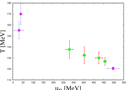
Figure 4: Average particle emission temperature $\overline{\langle T\rangle}$ and chemical potential $\overline{\langle\mu_{B}\rangle}$ at $E_{\rm Lab}/A=20$, 30, 40, 80, 158 GeV (CERN-SPS) and $\surd s_{NN}=130$ and 200 GeV (BNL-RHIC), from right to left (symbols). The “error bars” indicate the RMS deviations over particle species (i.e. $\delta\langle T\rangle$ and $\delta\langle\mu_{B}\rangle$). For SPS-20 and RHIC, these are depicted by dotted lines since the inhomogeneities are not statistically significant.

Fig. 4 depicts the energy dependence of the average freeze-out temperature and chemical potential, as defined in eq. (14). The general trend is the same as in the homogeneous model: $\overline{\langle T\rangle}$ increases with energy, while $\overline{\langle\mu_{B}\rangle}$ decreases. Their values agree to within $\sim 15\%$ with those for a homogeneous system obtained previously by others (cf. for example fig. 3 in Redlich et al. or fig. 27 in Braun-Munzinger et al. thermo ). The inhomogeneous model, however, predicts sizeable variations of the emission temperatures of different particle species: this is indicated in fig. 4 by the “error bars”, which correspond to $\delta\langle T\rangle$ and $\delta\langle\mu_{B}\rangle$ as defined in eq. (15). They were obtained from the best fit at each energy, i.e. using the parameters corresponding to the lowest $\chi^{2}/dof$ from the inhomogeneous model. We repeat, however, that at the lowest and highest energies the inhomogeneous fit has no statistical significance, in that $\chi^{2}/dof$ is only marginally better than for the homogeneous model. Hence, at these energies, the resulting $\delta\langle T\rangle$ and $\delta\langle\mu_{B}\rangle$ (dotted lines) should be taken with $\sim 100\%$ error.

At intermediate and high SPS energies, however, the variance of the temperature can be determined reasonably well and is significantly larger than zero. $\delta\langle T\rangle$ appears to be rather large already at $E_{\rm Lab}/A=30$ GeV, and increases further towards higher SPS energies. As already stated, $\chi^{2}(\delta\mu_{B})$ is rather flat for all energies, so that $\delta\langle\mu_{B}\rangle$ should also be taken with some uncertainty.

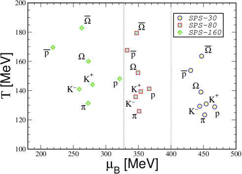
Figure 5: Freeze-out temperatures $\langle T\rangle_{i}$ and chemical potentials $\langle\mu_{B}\rangle_{i}$ of various particle species at $E_{\rm Lab}/A=30$, 80, 158 GeV.

Fig. 5 shows the freeze-out temperatures and chemical potentials for individual particle species at selected energies in the CERN-SPS range. The effect of the inhomogeneities is evident. For example, anti-protons are typically emitted from regions with lower baryon-chemical potential than protons; also, heavy particles are concentrated in “hot spots” while light pions are distributed more evenly throughout the decoupling volume etc. The temperatures of rare particle species can deviate much more from $\overline{\langle T\rangle}$ than $\delta\langle T\rangle$ from fig. 4 might suggest. This is, of course, due to their small weight in eq. (15). Finally, we note that the rather high temperatures of the hot spots from which the heavy particles emerge might indicate the need for a better treatment of interactions thermo_int than the simple excluded-volume model employed here.

V Summary and Outlook

We have shown that inhomogeneities on the freeze-out hypersurface do not average out but reflect in the 4$\pi$ (or midrapidity), single-inclusive abundances of various particle species. This is due to the non-linear dependence of the hadron densities $\rho_{i}(T,\mu_{B})$ on the local temperature and baryon-chemical potential. Consequently, even the average $\overline{\rho}_{i}$ probe higher moments of the $T$ and $\mu_{B}$ distributions. Searching for such inhomogeneities could represent a promising observable for a first-order phase transition.

We introduced a simple model for the statistical description of chemical freeze-out, extending the commonly used grand-canonical ensemble to the case of inhomogeneous decoupling surfaces. If freeze-out occurs shortly after a first-order phase transition, hydrodynamic flow and diffusion Bower:2001fq ; diff may not completely wash out inhomogeneities produced in the course of the phase transition. Given that the number of such “domains” is expected to be large, the inclusive distribution of temperature and baryon-chemical potential on the decoupling surface should be approximately Gaussian.

The model improves the fits of the measured particle ratios in the CERN-SPS energy regime $E_{\rm Lab}/A\simeq 30-160$ GeV significantly. Homogeneous freeze-out is well outside the 95.4% confidence interval. This suggests that at intermediate energies the freeze-out surface is not well “stirred”. Future studies could perhaps shed more light on whether these inhomogeneities can indeed be interpreted as fingerprints of a first-order phase transition. Eventually, one would want to establish more quantitative relations between the amplitudes of the $T$, $\mu_{B}$ inhomogeneities and the properties of the phase transition, e.g. its latent heat and interface tension. Furthermore, the role of inhomogeneities in the net-strangeness distribution should be studied. On the other hand, within the present model, no statistically significant improvement over homogeneous freeze-out was observed at lower (SPS-20) and higher (RHIC) energies.

Inhomogeneities could also affect the coalescence probabilities of (anti-) nucleons to light (anti-) nuclei, which are also sensitive to density perturbations ioffe . Other signals, such as two-particle correlations spherio ; bubble , could also be analyzed in this regard.

To improve the quality of the statistical fits, more data on hadron multiplicities would be helpful, in particular at the lower end of the CERN-SPS energy spectrum and at RHIC. This includes estimates of multiplicities of unstable resonances ($\rho$, $K^{*}$, $\omega$, $\Delta$ …) at chemical freeze-out reson . Data from GSI-FAIR and CERN-LHC will provide additional constraints for the evolution of chemical freeze-out with energy.

Note added: While we finished this manuscript, the superstatistics approach SuperStat was brought to our attention. It considers non-equilibrium systems in stationary states with fluctuating intensive quantities, which are described by a superposition of Boltzmann ensembles. Although our approach emerged from a different physical picture, it can nevertheless be viewed as an application of “superstatistics” to particle freeze-out in heavy-ion collisions.

Acknowledgements

We thank C. Greiner for fruitful remarks concerning the model, C. Blume and M. Gazdzicki for helpful discussions about the NA49 data and A. Grunfeld for helping with the construction of the resonance table. L.P. thanks CAPES for supporting a one-year stay at ITP, Goethe University. A.D. and D.Z. acknowledge the hospitality of the Nuclear Theory group during a stay at UFRJ sponsored by DAAD (PROBRAL program), where this work was completed. This work used computational resources provided by the Center for Scientific Computing (CSC) of Goethe University, Frankfurt.

References

- (1) H. Stöcker et al., Nucl. Phys. A 566 (1994) 15c; Nucl. Phys. A 590 (1995) 271c;
- (2) Z. Fodor and S. D. Katz, JHEP 0404 (2004) 050.
- (3) M. Stephanov, K. Rajagopal and E. V. Shuryak, Phys. Rev. Lett. 81, (1998) 4816.
- (4) D. Bower and S. Gavin, Phys. Rev. C 64 (2001) 051902.
- (5) K. Paech and A. Dumitru, Phys. Lett. B 623 (2005) 200; K. Paech, H. Stöcker and A. Dumitru, Phys. Rev. C 68 (2003) 044907; O. Scavenius, A. Dumitru and A. D. Jackson, arXiv:hep-ph/0103219, figs. 5,6.
-
(6)
http://map.gsfc.nasa.gov/m_mm.html
- (7) M. Gyulassy, D. H. Rischke and B. Zhang, Nucl. Phys. A 613 (1997) 397; M. Bleicher et al., Nucl. Phys. A 638 (1998) 391; H. J. Drescher, S. Ostapchenko, T. Pierog and K. Werner, Phys. Rev. C 65 (2002) 054902.
- (8) O. J. Socolowski, F. Grassi, Y. Hama and T. Kodama, Phys. Rev. Lett. 93 (2004) 182301.
- (9) A. Andronic, P. Braun-Munzinger and J. Stachel, arXiv:nucl-th/0511071.
- (10) see for example K. Redlich, J. Cleymans, H. Oeschler and A. Tounsi, Acta Phys. Polon. B 33 (2002) 1609; P. Braun-Munzinger, K. Redlich and J. Stachel, arXiv:nucl-th/0304013; M. Michalec, arXiv:nucl-th/0112044; and references therein.
- (11) J. Rafelski, Phys. Lett. B 262 (1991) 333; J. Rafelski, J. Letessier and A. Tounsi, Acta Phys. Polon. B 27 (1996) 1037; F. Becattini, J. Cleymans, A. Keranen, E. Suhonen and K. Redlich, Phys. Rev. C 64 (2001) 024901; F. Becattini, M. Gazdzicki, A. Keranen, J. Manninen and R. Stock, Phys. Rev. C 69 (2004) 024905; G. Torrieri, S. Steinke, W. Broniowski, W. Florkowski, J. Letessier and J. Rafelski, arXiv:nucl-th/0404083; S. Wheaton and J. Cleymans, arXiv:hep-ph/0412031; J. Letessier and J. Rafelski, arXiv:nucl-th/0504028.
- (12) F. Becattini, J. Manninen and M. Gazdzicki, arXiv:hep-ph/0511092.
- (13) D. Zschiesche, S. Schramm, J. Schaffner-Bielich, H. Stöcker and W. Greiner, Phys. Lett. B 547 (2002) 7; W. Florkowski, W. Broniowski and M. Michalec, Acta Phys. Polon. B 33 (2002) 761; D. Zschiesche, G. Zeeb, K. Paech, H. Stöcker and S. Schramm, J. Phys. G 30 (2004) S381; K. Paech et al., Acta Phys. Hung. A 21, 151 (2004).
- (14) B. Berdnikov and K. Rajagopal, Phys. Rev. D 61 (2000) 105017; K. Paech, Eur. Phys. J. C 33 (2004) S627.
- (15) A. Dumitru and R. D. Pisarski, Phys. Lett. B 504 (2001) 282; Nucl. Phys. A 698 (2002) 444.
- (16) L. Van Hove, Z. Phys. C 21 (1983) 93; M. Gyulassy, K. Kajantie, H. Kurki-Suonio and L. D. McLerran, Nucl. Phys. B 237 (1984) 477; L. P. Csernai and J. I. Kapusta, Phys. Rev. D 46 (1992) 1379.
- (17) O. Scavenius, A. Dumitru, E. S. Fraga, J. T. Lenaghan and A. D. Jackson, Phys. Rev. D 63 (2001) 116003; E. S. Fraga and R. Venugopalan, PhysicaA 345 (2004) 121; Braz. J. Phys. 34 (2004) 315.
- (18) I. N. Mishustin, Phys. Rev. Lett. 82 (1999) 4779.
- (19) see, for example, J. F. Lara, Phys. Rev. D 72 (2005) 023509 for a recent discussion of BBN in an inhomogeneous early universe, and for links to earlier literature.
- (20) S. A. Bass et al., Phys. Rev. C 60 (1999) 021902; Phys. Rev. C 61 (2000) 064909; Phys. Lett. B 460 (1999) 411; S. Soff, S. A. Bass and A. Dumitru, Phys. Rev. Lett. 86 (2001) 3981; D. Teaney, J. Lauret and E. V. Shuryak, arXiv:nucl-th/0110037; C. Nonaka and S. A. Bass, arXiv:nucl-th/0510038; T. Hirano, U. W. Heinz, D. Kharzeev, R. Lacey and Y. Nara, arXiv:nucl-th/0511046.
- (21) H. Sorge, Phys. Lett. B 373 (1996) 16.
- (22) P. Braun-Munzinger, J. Stachel and C. Wetterich, Phys. Lett. B 596 (2004) 61.
- (23) D. Adamova et al. [CERES Collaboration], Phys. Rev. Lett. 90 (2003) 022301.
- (24) section II in J. Cleymans and K. Redlich, Phys. Rev. C 60 (1999) 054908; for the general argument for ratios see e.g. eqs. (1-3) in M. Bleicher et al., Phys. Rev. C 59 (1999) 1844.
- (25) P. Braun-Munzinger, I. Heppe, J. Stachel, Phys. Lett. B 465 (1999) 15.
- (26) C. Höhne (for the NA49 collaboration), nucl-ex/0510049. Our present best fit (of the ratios) for the inhomogeneous model without independent fluctuations of yields at GeV, for example, versus 0.76 for (without contributions from weak decays).
- (27) M. Gazdzicki et al. [NA49 Collaboration], J. Phys. G 30 (2004) S701 [arXiv:nucl-ex/0403023]; A. Richard [NA49 Collaboration], J. Phys. G 31, S155 (2005); C. Blume [NA49 Collaboration], J. Phys. G 31, S685 (2005) [arXiv:nucl-ex/0411039]; C. Alt et al. [The NA49 Collaboration], J. Phys. G 30, S119 (2004) [arXiv:nucl-ex/0305017]; S. V. Afanasiev et al. [The NA49 Collaboration], Phys. Rev. C 66, 054902 (2002) [arXiv:nucl-ex/0205002]; T. Anticic et al., Phys. Rev. C 69, 024902 (2004); S. V. Afanasiev et al., Nucl. Phys. A 715 (2003) 161 [arXiv:nucl-ex/0208014]; T. Anticic et al. [NA49 Collaboration], Phys. Rev. Lett. 93, 022302 (2004) [arXiv:nucl-ex/0311024]; C. Meurer [NA49 Collaboration], J. Phys. G 30, S1325 (2004) [arXiv:nucl-ex/0406016]; M. Mitrovski [NA49 Collaboration], arXiv:nucl-ex/0406011; C. Alt et al. [NA49 Collaboration], Phys. Rev. Lett. 94, 192301 (2005) [arXiv:nucl-ex/0409004]; S. V. Afanasev et al. [NA49 Collaboration], Phys. Lett. B 491, 59 (2000); A. Mischke et al., Nucl. Phys. A 715, 453 (2003) [arXiv:nucl-ex/0209002]; V. Friese [NA49 Collaboration], Nucl. Phys. A 698, 487 (2002); S. V. Afanasiev et al. [NA49 Collaboration], Phys. Lett. B 538, 275 (2002) [arXiv:hep-ex/0202037]; S. V. Afanasiev et al. [NA49 Collaboration], Phys. Lett. B 538, 275 (2002) [arXiv:hep-ex/0202037].
- (28) J. Adams et al. [STAR Collaboration], arXiv:nucl-ex/0311017; M. Calderon de la Barca Sanchez, arXiv:nucl-ex/0111004; C. Adler et al. [STAR Collaboration], Phys. Rev. Lett. 89 (2002) 092301 [arXiv:nucl-ex/0203016]; C. Adler et al. [STAR Collaboration], Phys. Lett. B 595 (2004) 143 [arXiv:nucl-ex/0206008]; C. Adler et al. [STAR Collaboration], Phys. Rev. C 66 (2002) 061901 [arXiv:nucl-ex/0205015]; C. Adler et al. [STAR Collaboration], Phys. Rev. Lett. 87 (2001) 262302 [arXiv:nucl-ex/0110009]; C. Adler et al. [the STAR Collaboration], Phys. Rev. Lett. 86 (2001) 4778 [Erratum-ibid. 90 (2003) 119903] [arXiv:nucl-ex/0104022]; C. Adler et al., Phys. Rev. C 65 (2002) 041901. J. Castillo [STAR Collaboration], Nucl. Phys. A 715 (2003) 518 [arXiv:nucl-ex/0210032]; J. Adams et al. [STAR Collaboration], Phys. Rev. Lett. 92 (2004) 182301 [arXiv:nucl-ex/0307024]; J. Adams et al. [STAR Collaboration], Phys. Lett. B 567 (2003) 167 [arXiv:nucl-ex/0211024]; C. Suire [STAR Collaboration], Nucl. Phys. A 715 (2003) 470 [arXiv:nucl-ex/0211017].
- (29) J. Cleymans, B. Kämpfer, M. Kaneta, S. Wheaton and N. Xu, Phys. Rev. C 71 (2005) 054901.
- (30) O. Barannikova [STAR Collaboration], arXiv:nucl-ex/0403014; J. Adams et al. [STAR Collaboration], arXiv:nucl-ex/0501009; J. Adams et al. [STAR Collaboration], Phys. Rev. Lett. 92 (2004) 112301 [arXiv:nucl-ex/0310004];
- (31) S. Eidelman et al. [Particle Data Group Collaboration], Phys. Lett. B 592 (2004) 1.
- (32) For SPS-158 only the fit is shown; restricting the homogeneous fit to the mid-rapidity data gives smaller , but still significantly higher than in the inhomogeneous approach. is smaller if other particle ratios are considered, as for example instead of Pbm05 or if finite widths of resonances are taken into account Becc05 . However, the increase of at SPS energies is generic if Na49 -data are fitted.
- (33) D. Zschiesche, arXiv:nucl-th/0505054, fig. 7.
- (34) E. V. Shuryak and M. A. Stephanov, Phys. Rev. C 63 (2001) 064903; M. Abdel-Aziz and S. Gavin, Phys. Rev. C 70 (2004) 034905.
- (35) see e.g. eq. (30) in B. L. Ioffe, I. A. Shushpanov and K. N. Zyablyuk, Int. J. Mod. Phys. E 13 (2004) 1157;
- (36) H. Heiselberg and A. D. Jackson, arXiv:nucl-th/9809013; S. J. Lindanbaum, R. S. Longacre and M. Kramer, arXiv:nucl-th/0304082; W. N. Zhang, S. X. Li, C. Y. Wong and M. J. Efaaf, Phys. Rev. C 71 (2005) 064908.
- (37) C. Markert, J. Phys. G 31 (2005) S169.
- (38) C. Beck, Phys. Rev. Lett. 87 (2001) 180601; C. Beck and E. G. D. Cohen, Physica A 322 (2003) 267; H. Touchette and C. Beck, Phys. Rev. E 71 (2005) 016131.