Neutron structure effects in the deuteron and one neutron halos

Abstract

Although the neutron ($n$) does not carry a total electric charge, its charge and magnetization distributions represented in momentum space by the electromagnetic form factors, $F_{1}^{(n)}(q^{2})$ and $F_{2}^{(n)}(q^{2})$, lead to an electromagnetic potential of the neutron. Using this fact, we calculate the electromagnetic corrections to the binding energy, $B_{d}$, of the deuteron and a one neutron halo nucleus (¹¹Be), by evaluating the neutron-proton and the neutron-charged core (¹⁰Be) potential, respectively. The correction to $B_{d}$ ($\sim 9$ keV) is comparable to that arising due to the inclusion of the $\Delta$-isobar component in the deuteron wave function. In the case of the more loosely bound halo nucleus, ¹¹Be, the correction is close to about $2$ keV.

I Introduction

Studying the sub-structures of nuclei and nucleons, encoded either in elastic electromagnetic form factors or deep inelastic structure functions, has been a field of continued interest in nuclear and particle physics. In this paper we shall focus on the aspect of nucleon substructure in connection with the appearance and relevance of electromagnetic form factors in nuclear physics. We shall calculate the electromagnetic contributions to the binding energies of loosely bound neutron-nucleus systems, arising due to the neutron form factors. Such systems are realized by the deuteron and the one-neutron halo nuclei. Recently, the availability of radioactive beams opened up the possibility to study the structure of unstable nuclei. Such experiments tani revealed neutron rich nuclei whose spatial extensions are very large as compared to the range of the nuclear force. These so-called “halo” nuclei consist of very loosely bound valence neutrons which tunnel to distances far from the remaining set of nucleons. Such nuclei can be viewed as a system of a “core” with normal nuclear density and a low density halo of one or more neutrons. Thus one expects that the neutrons in the halo do not experience the strong force due to individual nucleons in the core but rather interact with the core as a whole. Based on this understanding, many few body models have been constructed and elaborately refined over the past few years filo ; others in order to explain a variety of experimental data.

It is well known by now that the neutron does have structure and hence an electric charge distribution which can be measured in elastic electron-nucleon scattering experiments. The interest in this field was revived due to the new experimental results on the nucleon form factor from the Jefferson laboratory jone . Considering the recent interest in nucleon form factors along with the experimental advances being made in halo nuclear studies, we found it timely to investigate the role of the neutron structure in the deuteron and one-neutron halo nuclei. In what follows, we shall derive an expression for the electromagnetic potential between the neutron and a charged particle (generalizing hereby the Breit equation by adding to it the finite size corrections) and then apply it to determine the perturbative corrections to the binding energy of nuclei.

II The neutron electromagnetic potential

There exists a well known prescription for obtaining a potential from quantum field theory lali4 ; fein . The method consists of taking the Fourier transform of a non-relativistic scattering amplitude, say $M_{NR}$, for a scattering process of the type $AB\rightarrow AB$. Since the method is completely general, one can handle simple cases with an amplitude which corresponds to one or two particle exchange diagrams or consider more complicated cases where the amplitude needs to be calculated using higher order corrections in the perturbative Feynman-Dyson expansion. If the amplitude depends only on the magnitude of momentum transfer ($Q$) in the process, then the Fourier transform to obtain the potential, $V(r)$, reduces to marek1 :

$$V(r)={1\over(2\pi)^{3}}{1\over r}4\pi\,\int_{0}^{\infty}\,dQ\,Q\,\,M_{NR}(Q^{2})\,\sin(Qr)\,.$$ (1)

Obviously, if $M_{NR}(Q^{2})\propto 1/Q^{2}$ (non-relativistic propagator of a massless particle), the potential is proportional to $1/r$. Some examples of exotic potentials derived from quantum field theory can be found in fein ; marek1 ; casi .

The aim of the present work is to study the role of the neutron structure in neutron - charged particle interactions. Hence we shall be interested in obtaining an electromagnetic potential which describes the interaction between the charged particle and the neutron. To obtain this potential, we shall start with the scattering amplitude for the process $n+A\rightarrow n+A$, where $A$ can be any charged particle with charge $Ze$ (with $Z$ a positive integer). We shall consider two cases: the neutron (spin 1/2) + A (spin 1/2) and neutron (spin 1/2) + A (spin 0) case with the former being relevant for the neutron-proton system (deuteron) and the latter for the one-neutron halo ¹¹Be taken as a neutron plus a ¹⁰Be core in the $s$-state.

Mathematically, the complete spin-$1/2$ fermion vertex (fermion-photon-fermion) is given as marek3 :

$${\cal O}^{\mu} = F_{1}(q^{2})\,\gamma^{\mu}\,+\,{i\sigma_{\mu\nu}\over 2m_{f}}\,q_{\nu}\,F_{2}(q^{2})\,+i\epsilon^{\mu\nu\alpha\beta}{\sigma_{\alpha\beta}\over 4m_{f}}\,q_{\nu}\,F_{3}(q^{2})$$ (2)

$$+ {1\over 2m_{f}}\,\biggl{(}q^{\mu}\,-\,{q^{2}\over 2m_{f}}\gamma^{\mu}\biggr{)}\,\gamma_{5}\,F_{4}(q^{2})~{},$$

where the sub-structure of the fermion is contained in the various form factors, $F_{i}$ ($i=1,2,3,4$). $q_{\mu}$ is the four-momentum carried by the photon ($q^{2}=q^{\mu}q_{\mu}$), $m_{f}$ is the mass of the fermion and the $\gamma$’s are the usual Dirac matrices bjor . The four-momentum squared, $q^{2}=\omega^{2}-\vec{Q}^{2}$ (where $\omega$ is the energy and $\vec{Q}$ the three momentum), reduces in the non-relativistic limit ($\omega\sim 0$) to $q^{2}=-\vec{Q}^{2}$. The above four form factors appear in the expression for the cross section for electron-nucleon elastic scattering and the nucleon form factors are thus extracted from such scattering experiments. The first form factor, $F_{1}$ is connected to the charge distribution inside the nucleon and $F_{1}(0)=$ the total charge of the nucleon. The form factors $F_{2}$, $F_{3}$ and $F_{4}$ are related to the anomalous magnetic moment, electric dipole and Zeldovich anapole moment, respectively. In what follows, we shall obtain the electromagnetic potential for the spin-1/2 - spin-1/2 and the spin-1/2 - spin-0 case in terms of the nucleon electromagnetic form factors $F_{1}(q^{2})$ and $F_{2}(q^{2})$ as the other form factors ($F_{3}(q^{2})$ and $F_{4}(q^{2})$) are related to the weak interaction and their effects are small.

II.1 The neutron proton case

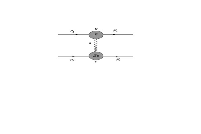
Figure 1: Feynman diagram for neutron scattering from a nucleus with $Z$ being the number of protons.

In order to perform a complete calculation of the potential, we turn to the task of expanding the amplitude in $1/c^{2}$ terms, thereby generalizing the Breit equation lali4 by the inclusion of two electromagnetic form factors. This will lead to non-local and spin-dependent terms in the potential whose contributions to the binding energies are not negligible as will be seen later. Starting with the Feynman diagram of Fig. 1, the nucleon-photon-nucleon vertices in terms of the nucleon form factors $F_{1}$ and $F_{2}$ can be written as,

$$\Gamma_{X}^{\mu} = F_{1}^{X}\,\gamma^{\mu}\,\,-\,\,{\sigma^{\mu\nu}\over 2M_{X}\,c}\,q_{\nu}\,F_{2}^{X}$$ (3)

$$\Gamma_{Y}^{\mu} = F_{1}^{Y}\,\gamma^{\mu}\,\,+\,\,{\sigma^{\mu\nu}\over 2M_{Y}\,c}\,q_{\nu}\,F_{2}^{Y}\,.$$

The photon momentum, $q=P_{1}^{\prime}-P_{1}=P_{2}-P_{2}^{\prime}$. In the non-relativistic limit ($q^{0}=0$), $q^{2}=-\vec{Q}^{2}$, where, $\vec{Q}=\vec{p}_{1}^{\,\,\prime}-\vec{p}_{1}=\vec{p}_{2}-\vec{p}_{2}^{\,\,\prime}$. The amplitude for the process $N+N\rightarrow N+N$ is then given by lali4 ,

$$M_{fi}=e_{X}\,e_{Y}\,\biggl{[}\,\biggl{(}\bar{u}(\vec{p}_{1}^{\,\,\prime})\,\Gamma_{X}^{\mu}\,u(\vec{p}_{1})\biggr{)}\,\,D_{\mu\nu}(\vec{Q})\,\,\biggl{(}\bar{u}(\vec{p}_{2}^{\,\,\prime})\,\Gamma_{Y}^{\nu}\,u(\vec{p}_{2})\biggr{)}\,\biggr{]}\,\,,$$ (4)

where, $D_{\mu\nu}(\vec{Q})$ is the photon propagator and $u(\vec{p}_{1})$, $u(\vec{p}_{2})$ etc., the usual Dirac spinors given as,

$$u\,=\,\sqrt{2M}\left[\begin{array}[]{c}{\displaystyle\biggl{(}1-{\vec{p}^{\,2}\over 8M^{2}c^{2}}\biggr{)}\,w}\\[5.0pt] {\displaystyle{\vec{\sigma}\cdot\vec{p}\over 2Mc}\,w}\end{array}\right]\,.$$ (5)

Substituting for the $u(\vec{p})$’s and the vertex factors given above, the amplitude is evaluated and then rearranged to be written in the following form:

$$M_{fi}=-2\,M_{X}\,\cdot\,2\,M_{Y}\,[w_{1}^{\prime*}\,w_{2}^{\prime*}\,\,U(\vec{p}_{1},\vec{p}_{2},\vec{Q})\,w_{1}\,w_{2}\,]\,,$$ (6)

thus obtaining the potential $U(\vec{p}_{1},\vec{p}_{2},\vec{Q})$ in momentum space. The potential in $r$-space is obtained simply from a Fourier transform of the potential in momentum space, namely,

$$V(\vec{r})\,=\,\int\,e^{i\vec{Q}\cdot\vec{r}}\,\,U(\vec{p}_{1},\vec{p}_{2},\vec{Q})\,\,{d^{3}q\over(2\,\pi)^{3}}\,\,.$$ (7)

The electromagnetic neutron-proton potential in momentum space, using the above procedure is found to be,

$$U^{np}(\vec{p}_{1},\vec{p}_{2},\vec{Q})=4\pi e^{2}\,\biggl{\{}\,F_{1}^{n}\,F_{1}^{p}\,\biggl{[}\,{1\over\vec{Q}^{2}}\,-\,{1\over 8\,M_{n}^{2}\,c^{2}}\,-\,{1\over 8\,M_{p}^{2}\,c^{2}}\,-\,{\vec{\sigma}_{1}\cdot\vec{\sigma}_{2}\over 4\,M_{n}\,M_{p}\,c^{2}}$$

$$+\,\,{(\vec{\sigma}_{1}\cdot\vec{Q})(\vec{\sigma}_{2}\cdot\vec{Q})\over 4\,M_{n}\,M_{p}\,c^{2}\vec{Q}^{2}}+\,{i\vec{\sigma}_{1}\cdot(\vec{Q}\times\vec{p}_{1})\over 4\,M_{n}^{2}\,c^{2}\,\vec{Q}^{2}}\,-\,{i\vec{\sigma}_{2}\cdot(\vec{Q}\times\vec{p}_{2})\over 4\,M_{p}^{2}\,c^{2}\,\vec{Q}^{2}}\,+\,{i\vec{\sigma}_{2}\cdot(\vec{Q}\times\vec{p}_{1})\over 2\,M_{p}\,M_{n}\,c^{2}\,\vec{Q}^{2}}\,-\,{i\vec{\sigma}_{1}\cdot(\vec{Q}\times\vec{p}_{2})\over 2\,M_{p}\,M_{n}\,c^{2}\,\vec{Q}^{2}}$$

$$-\,{\vec{p}_{1}\cdot\vec{p}_{2}\over M_{n}\,M_{p}\,c^{2}\,\vec{Q}^{2}}\,+\,{(\vec{p}_{1}\cdot\vec{Q})\,(\vec{p}_{2}\cdot\vec{Q})\over M_{n}\,M_{p}\,c^{2}\,\vec{Q}^{4}}\,\biggr{]}$$

$$+\,F_{1}^{n}\,F_{2}^{p}\,\biggl{[}\,-\,{1\over 4\,M_{p}^{2}\,c^{2}}\,-\,{\vec{\sigma}_{1}\cdot\vec{\sigma}_{2}\over 4\,M_{n}\,M_{p}\,c^{2}}\,+\,\,{(\vec{\sigma}_{1}\cdot\vec{Q})(\vec{\sigma}_{2}\cdot\vec{Q})\over 4\,M_{n}\,M_{p}\,c^{2}\vec{Q}^{2}}\,+\,{i\vec{\sigma}_{2}\cdot(\vec{Q}\times\vec{p}_{1})\over 2\,M_{p}\,M_{n}\,c^{2}\,\vec{Q}^{2}}\,-\,{i\vec{\sigma}_{2}\cdot(\vec{Q}\times\vec{p}_{2})\over 2\,M_{p}^{2}\,c^{2}\,\vec{Q}^{2}}\,\biggr{]}$$

$$+\,F_{2}^{n}\,F_{1}^{p}\,\biggl{[}\,-\,{1\over 4\,M_{n}^{2}\,c^{2}}\,-\,{\vec{\sigma}_{1}\cdot\vec{\sigma}_{2}\over 4\,M_{n}\,M_{p}\,c^{2}}\,+\,\,{(\vec{\sigma}_{1}\cdot\vec{Q})(\vec{\sigma}_{2}\cdot\vec{Q})\over 4\,M_{n}\,M_{p}\,c^{2}\vec{Q}^{2}}\,-\,{i\vec{\sigma}_{1}\cdot(\vec{Q}\times\vec{p}_{2})\over 2\,M_{p}\,M_{n}\,c^{2}\,\vec{Q}^{2}}\,+\,{i\vec{\sigma}_{1}\cdot(\vec{Q}\times\vec{p}_{1})\over 2\,M_{n}^{2}\,c^{2}\,\vec{Q}^{2}}\,\biggr{]}$$

$$+\,F_{2}^{n}\,F_{2}^{p}\,\biggl{[}\,-\,{\vec{\sigma}_{1}\cdot\vec{\sigma}_{2}\over 4\,M_{n}\,M_{p}\,c^{2}}\,+\,\,{(\vec{\sigma}_{1}\cdot\vec{Q})(\vec{\sigma}_{2}\cdot\vec{Q})\over 4\,M_{n}\,M_{p}\,c^{2}\vec{Q}^{2}}\,\biggr{]}\,\,\biggr{\}}\,.$$ (8)

In obtaining the above expression, we have dropped terms of order higher than ($1/c^{2}$). The above expression involves a separate $1/c^{2}$ expansion corresponding to each of the form factor combinations. This is to say, the term proportional to $F_{1}^{n}F_{1}^{p}/Q^{2}$ is the leading term of the coupling constants combination $F_{1}^{n}F_{1}^{p}$, whereas the other terms proportional to this combination are $1/c^{2}$ suppressed. However, we cannot say that just like the ($1/c^{2}$) terms in $F_{1}^{n}F_{1}^{p}$, those in the other combinations like $F_{1}^{n}F_{2}^{p}$, $F_{2}^{n}F_{1}^{p}$ and $F_{2}^{n}F_{2}^{p}$ are also suppressed, as the latter represent different combinations of coupling constants. Indeed, all combinations different from $F_{1}^{n}F_{1}^{p}$ are displayed also in the leading order albeit they appear with the $1/c^{2}$ factor which does not imply that they are smaller than $F_{1}^{n}F_{1}^{p}/Q^{2}$. We will see later how this works in practice. The constant $e$ in the above is defined such that $e^{2}=\alpha$, the fine structure constant. Since the experimental form factors for the neutron as well as the proton are normalized in a similar way, we have a vertex factor of $\sqrt{4\pi\alpha}$ at the neutron-photon-neutron vertex too, in order to remove the extra factor by which the experimental neutron form factor was divided.

The detailed calculation of the Fourier transforms of the terms in (II.1) and the corresponding potential in $r$-space is given in the appendix. The terms which appear with cross products of momenta in (II.1), do not contribute to the binding energy correction for the deuteron, as shown in the appendix.

II.2 The neutron spin-zero-nucleus case

To evaluate the electromagnetic potential between the neutron and a spin-zero nucleus, we repeat a very similar procedure as above, with the vertex $Y$ in Fig. 1 replaced in this case by,

$$\Gamma_{Y}^{\nu}=F^{Y}(q^{2})\,(P_{2}+P_{2}^{\prime})^{\nu}\,,$$ (9)

where, $F^{Y}(q^{2})$ is the form factor of the nucleus ($A$) in momentum space. We also replace the appropriate normalization for the spin zero particles. The potential in momentum space is found to be,

$$U^{nA}(\vec{p}_{1},\vec{p}_{2},\vec{Q})=4\pi e^{2}\,\biggl{\{}\,F_{1}^{n}\,F^{Y}\,\biggl{[}\,{1\over\vec{Q}^{2}}\,-\,{1\over 8\,M_{n}^{2}\,c^{2}}\,-\,{\vec{p}_{1}\cdot\vec{p}_{2}\over M_{n}\,M_{A}\,c^{2}\,\vec{Q}^{2}}+\,{(\vec{p}_{1}\cdot\vec{Q})\,(\vec{p}_{2}\cdot\vec{Q})\over M_{n}\,M_{A}\,c^{2}\,\vec{Q}^{4}}$$

$$+\,{i\vec{\sigma}_{1}\cdot(\vec{Q}\times\vec{p}_{1})\over 4\,M_{n}^{2}\,c^{2}\,\vec{Q}^{2}}\,-\,{i\vec{\sigma}_{1}\cdot(\vec{Q}\times\vec{p}_{2})\over 2\,M_{A}\,M_{n}\,c^{2}\,\vec{Q}^{2}}\biggr{]}$$

$$+\,F_{2}^{n}\,F^{Y}\,\biggl{[}-\,{1\over 4\,M_{n}^{2}\,c^{2}}\,+\,{i\vec{\sigma}_{1}\cdot(\vec{Q}\times\vec{p}_{1})\over 2\,M_{n}^{2}\,c^{2}\,\vec{Q}^{2}}\,-\,{i\vec{\sigma}_{1}\cdot(\vec{Q}\times\vec{p}_{2})\over 2\,M_{A}\,M_{n}\,c^{2}\,\vec{Q}^{2}}\biggr{]}\,\biggr{\}}\,.$$ (10)

This potential will be used in the present work to evaluate the correction to the binding energy of the one-neutron halo nucleus, ¹¹Be, taken as a neutron plus ¹⁰Be core. The evaluation of the ¹¹Be wave function is usually done in a neutron plus ¹⁰Be core model where the ground state (spin zero) and an excited state (spin 2) of the core are considered. We shall restrict to assuming the core to be a spin zero nucleus since the calculation of a spin 1/2 - spin 2 electromagnetic potential is beyond the scope of the present work. The contributions of the spin-2 terms to the ¹¹Be wave function are in any case small and would have only a small overlap with the electromagnetic potential which is not long-ranged.

In the next sub-section, we shall describe the various parameterizations of the form factors which will be used to evaluate the above potentials.

II.3 The electromagnetic form factors $F_{1}(q^{2})$ and $F_{2}(q^{2})$

The form factors $F_{1}$ and $F_{2}$ have been extracted from several experiments and parameterized in different forms in the past gasi . However, a discrepancy between the old results and new experiments which extract the two form factors through polarization measurements was recently reported jone . It was found, however, that this discrepancy could be resolved by taking into account the two photon contribution chen . Therefore, in the following, we shall make use of the ‘standard’ parameterization of the form factors. Considering the renewed debate on the nucleon form factors, in the present work we shall also perform the calculations with different parameterizations available in the literature. The Sachs form factors $G_{E}$ and $G_{M}$ which appear in the expressions for the electron-nucleon elastic cross sections are related to the structure functions $F_{1}$ and $F_{2}$. The nucleon form factors $F_{1}^{N}(q^{2})$ and $F_{2}^{N}(q^{2})$ are thus given as

$$F_{1}^{N}(q^{2})={4M^{2}\,G_{E}^{N}(q^{2})\,-\,q^{2}\,G_{M}^{N}(q^{2})\over 4M^{2}\,-\,q^{2}}~{},$$ (11)

$$F_{2}^{N}(q^{2})={4M^{2}[\,G_{M}^{N}(q^{2})\,-\,G_{E}^{N}(q^{2})]\over 4M^{2}\,-\,q^{2}}$$

where $M$ is the mass of the nucleon and $q^{2}=\omega^{2}-\vec{Q}^{2}$ is the four momentum of the virtual photon as mentioned before. A large body of experiments starting from the sixties until now has been dedicated to the extraction of $G_{E}^{n}(q^{2})$ and $G_{M}^{n}(q^{2})$. Though the newer experiments have smaller statistical errors, there still exist uncertainties arising from the theoretical description of the deuteron. Hence, in the case of the neutron, we shall use different parameterizations available in literature.

II.3.1 The dipole form factor and the neutron electric potential

We shall use the following form for $G_{E}^{n}(q^{2})$ plat with different sets of parameters ‘$a$’ and ‘$b$’ obtained in literature:

$$G_{E}^{n}(q^{2})={a\,\mu_{n}\,(q^{2}/4M^{2})\over 1\,-\,b\,(q^{2}/4M^{2})}\,G_{D}(q^{2})~{},$$ (12)

where $\mu_{n}$ is the neutron magnetic moment and $G_{D}(q^{2})$ is the standard “dipole fit” which is generally used in summarizing the electron-nucleon elastic scattering data. With $G_{D}(q^{2})$ defined as

$$G_{D}(q^{2})={1\over(1\,-\,q^{2}/m^{2})^{2}}~{},$$ (13)

it was observed that

$$G_{E}^{p}(q^{2})\simeq{G_{M}^{p}(q^{2})\over\mu_{p}}\simeq{G_{M}^{n}(q^{2})\over\mu_{n}}\simeq G_{D}(q^{2})~{},$$ (14)

where the magnetic moments $\mu_{p}$ and $\mu_{n}$ of the proton and neutron (in nuclear magneton) are 2.79 and $-1.91$, respectively. Using the above definitions of $G_{E}^{n}(q^{2})$ and $G_{M}^{n}(q^{2})$ in (11), we obtain the following non-relativistic expression (i.e. with $q^{2}\simeq-\vec{Q}^{2}$) for the form factor $F_{1}^{n}(Q^{2})$:

$$F_{1}^{n}(Q^{2})=|\mu_{n}|\,Q^{2}\left[{4M^{2}\,(a-1)\,-\,Q^{2}b\over 4M^{2}\,+\,bQ^{2}}\right]\,\,{1\over 4M^{2}+Q^{2}}\,\,{1\over(1+Q^{2}/m^{2})^{2}}\,.$$ (15)

At this point, it is nice to note that using the dipole form factors, the potential between the structured neutron and an electron can be derived analytically and is given by,

$$V^{n}(r)={-Z\alpha\,|\mu_{n}|\over(1-b)}\,{1\over r}\,\,\biggl{[}\,(a-1)\,H_{1}^{n}\,-b\,H_{2}^{n}\,\biggr{]}~{},$$ (16)

where

$$H_{1}^{n}={1\over(\kappa^{2}-1)^{2}}\,e^{-\kappa mr}\,-\,{1\over(\kappa^{\prime 2}-1)^{2}}\,e^{-\kappa^{\prime}mr}$$ (17)

$$+ \left[{1\over(\kappa^{\prime 2}-1)^{2}}\,-\,{1\over(\kappa^{2}-1)^{2}}\right]\,e^{-mr}\,+\,{1\over 2}\,\left[{m\over(\kappa^{2}-1)}\,-\,{m\over(\kappa^{\prime 2}-1)}\right]\,r\,e^{-mr}$$

and

$$H_{2}^{n} = -{1\over(\kappa^{2}-1)^{2}}\,e^{-\kappa mr}\,+\,{1\over(\kappa^{\prime 2}-1)^{2}}\,\biggl{(}{\kappa^{\prime}\over\kappa}\biggr{)}^{2}\,e^{-\kappa^{\prime}mr}$$ (18)

$$- \,\left[{1\over(\kappa^{\prime 2}-1)^{2}}\,-\,{1\over(\kappa^{2}-1)^{2}}\right]\,{1\over\kappa^{2}}\,e^{-mr}\,$$

$$- \,\left[{1\over(\kappa^{2}-1)}\,-\,{1\over(\kappa^{\prime 2}-1)}\right]\,{1\over\kappa^{2}}\,e^{-mr}\biggl{(}{mr\over 2}-1\biggr{)}~{},$$

where $\kappa=2M/m$, $\kappa^{\prime}=\kappa/\sqrt{b}$ and typically $m^{2}=0.71$ GeV² gasi ; bosted .

In bosted , the neutron magnetic form factor was also fitted with the form

$${G_{M}^{n}(Q^{2})\over\mu_{n}}={1\over 1\,-\,1.74Q\,+\,9.29Q^{2}\,-\,7.63Q^{3}\,+\,4.63Q^{4}}~{},$$ (19)

and was shown to reproduce the existing data quite well. We shall perform calculations using this form of $G_{M}^{n}(Q^{2})$ and the dipole form of $G_{E}^{n}(Q^{2})$. In this case however, we evaluate the potential numerically and use it to evaluate the binding energy as explained in the next section.

II.3.2 The bump tail model

All new and old data of the electric and magnetic form factors of the proton and the neutron were recently re-analyzed by a fit walch based on a pion cloud model. A common feature (a bump) was noticed in the data at low momentum transfer, which the authors attributed to the existence of a pion cloud around a bare nucleon. The form factors were parameterized in terms of a bump on top of a large smooth part. Purely phenomenologically, the smooth part was parameterized with a superposition of two dipoles:

$$G_{S}(Q^{2})={a_{10}\over(1+Q^{2}/a_{11})^{2}}\,+\,{a_{20}\over(1+Q^{2}/a_{21})^{2}}$$ (20)

and the bump as a superposition of two Gaussians:

$$G_{b}(Q^{2})=\exp\biggl{[}-{1\over 2}\,\biggl{(}{Q-Q_{b}\over\sigma_{b}}\biggr{)}^{2}\,\biggr{]}\,\,+\exp\biggl{[}-{1\over 2}\,\biggl{(}{Q+Q_{b}\over\sigma_{b}}\biggr{)}^{2}\,\biggr{]}\,.$$ (21)

The neutron and proton, electric and magnetic form factors are then given by the ansatz,

$$G_{N}(Q^{2})=G_{S}(Q^{2})+a_{b}\,Q^{2}\,G_{b}(Q^{2})$$ (22)

where the parameter $a_{b}$ is essentially the amplitude of the bump. The parameters for the proton form factors are taken from Table II of walch and those for the neutron are taken from a more recent work glazier where the authors use a similar phenomenological fit. The neutron parameters fitted in glazier are within the error bars of those quoted in Table II of walch for the neutron.

II.4 The nuclear form factor

The form factor of ¹⁰Be is evaluated by taking the Fourier transform of a semiphenomenological nuclear charge density given in gambhir . Though the actual density of ¹⁰Be may have a complicated structure, the following form provided by the authors in gambhir is in very good agreement with experimental data on nuclear form factors. The charge density distribution is given as,

$$\rho(r)={\rho^{0}\over 1+[(1+(r/R)^{2})/2]^{\alpha}[e^{(r-R)/a}+e^{-(r+R)/a}]}\,,$$ (23)

where, $\rho^{0}$ is determined from the normalization condition:

$$4\pi\,\int\,\,\rho(r)\,r^{2}\,dr\,=\,Z\,,$$ (24)

with $Z$ being the total number of protons in the nucleus. The parameters for ¹⁰Be can be found in Table 1 of gambhir .

III Corrections to nuclear binding energies

As mentioned in the previous section, we evaluate the correction $\Delta E$ to the binding energy of the deuteron and the one-neutron halo nucleus ${}^{11}{\rm Be}$.

$$\Delta E=\int\,\Psi^{*}({\bf r})V^{n}(r)\Psi({\bf r})d{\bf r}\,,$$ (25)

where $\Psi$ is the wave function corresponding to the unperturbed Hamiltonian, $H_{0}$ (the total $H=H_{0}+V$).

III.1 The deuteron

In the deuteron case, we perform the calculation for the dominant $s$-state of the wave function obtained using the neutron-proton strong interaction. When the potential, $V^{n}(r)$, depends only on the magnitude of ${\bf r}$ and is spin-independent, the above equation reduces to the simple form:

$$\Delta E\,=\,\int_{0}^{\infty}\,r^{2}\,u^{2}(r)\,V^{n}(r)\,dr$$ (26)

where $u(r)$ is the radial part of the deuteron wave function. We use a parameterization of this wave function using the Paris nucleon-nucleon potential as given in paris . Since the Paris potential itself is written as a discrete superposition of Yukawa type terms, the wave function is parameterized in a similar way as:

$$u(r)=\sum_{j=1}^{13}C_{j}\,\exp(-m_{j}r)\,/\,r\,.$$ (27)

The coefficients $C_{j}$ with dimensions of [fm^-1/2] are listed in Table 1 of paris and the masses $m_{j}$ are given as $m_{j}=\alpha+(j-1)m_{0}$, with $m_{0}=1$ fm^-1 and $\alpha=0.2316$ fm^-1. In Table I, we list the corrections to the deuteron binding energy due to each of the terms in (II.1) using the most recent parameterization of Refs. walch and glazier . It can be seen that with the $F_{1}^{n}F_{1}^{p}$ combination of form factors, all terms other than the leading one are one or two orders of magnitude smaller as expected from the ($1/c^{2}$) expansion. The contributions of the terms involving $F_{2}^{n}(Q^{2})$ are large as compared to those with $F_{1}^{n}(Q^{2})$ simply due to the fact that unlike $F_{1}^{n}(Q^{2})$, $F_{2}^{n}(Q^{2})$ does not vanish as $Q^{2}\to 0$. Table I has been arranged according to the different form factor combinations to display in a clear way, the theoretical expectations discussed below Eq. (II.1). First, one should note that the entry corresponding to the $F_{1}^{n}F_{1}^{p}$ form factor combination has a leading term followed by ($1/c^{2}$) suppressed next-to-leading order terms. We have done this to display in this particular case, the significance of the next-to-leading order terms. In the next three combinations, only the leading terms of these particular combinations are listed. These terms contain a ($1/c^{2}$) factor which, however, does not make them always suppressed as compared to the leading term of the first combination $F_{1}^{n}F_{1}^{p}$, bearing in mind that we introduce a new momentum dependent coupling constant $F_{2}$. This is to say that one should not expect terms with different form factor combinations to give similar results. This is in agreement with the remarks we made regarding the $1/c$ expansion in section II.1.

Table 1: Corrections due to individual terms in the neutron-proton electromagnetic potential, to the deuteron binding energy in keV, using the parameterizations of form factors in walch ; glazier . The corrections assuming a point proton are listed in the last column.

Form factor	Term in $U^{np}(\vec{p}_{1},\vec{p}_{2},\vec{Q})$	$\Delta E$ (keV)	$\Delta E$ (keV)(with $F_{1}^{p}=1,F_{2}^{p}=\kappa_{p}$)
combination
$F_{1}^{n}\,F_{1}^{p}$	${\displaystyle{1\over\vec{q}^{\,2}}}$	$-1.25$	$-0.923$
	${\displaystyle-\,{1\over 8\,M_{n}^{2}\,c^{2}}\,-\,{1\over 8\,M_{p}^{2}\,c^{2}}}$	$-0.016$	$-0.049$
	${\displaystyle-\,{\vec{\sigma}_{1}\cdot\vec{\sigma}_{2}\over 4\,M_{n}\,M_{p}\,c^{2}}}$	$-0.016$	$-0.049$
	${\displaystyle{(\vec{\sigma}_{1}\cdot\vec{q})(\vec{\sigma}_{2}\cdot\vec{q})\over 4\,M_{n}\,M_{p}\,c^{2}\vec{q}^{\,2}}}$	$-0.028$	$-0.063$
	${\displaystyle-\,{\vec{p}_{1}\cdot\vec{p}_{2}\over M_{n}\,M_{p}\,c^{2}\,\vec{q}^{\,2}}}$	$-0.02$	0.053
	${\displaystyle{(\vec{p}_{1}\cdot\vec{q})\,(\vec{p}_{2}\cdot\vec{q})\over M_{n}\,M_{p}\,c^{2}\,\vec{q}^{\,4}}}$	$-0.05$	$-0.155$
$F_{1}^{n}\,F_{2}^{p}$	${\displaystyle-\,{1\over 4\,M_{p}^{2}\,c^{2}}}$	$-0.034$	$-0.177$
	${\displaystyle-\,{\vec{\sigma}_{1}\cdot\vec{\sigma}_{2}\over 4\,M_{n}\,M_{p}\,c^{2}}}$	$-0.034$	$-0.177$
	${\displaystyle{(\vec{\sigma}_{1}\cdot\vec{q})(\vec{\sigma}_{2}\cdot\vec{q})\over 4\,M_{n}\,M_{p}\,c^{2}\vec{q}^{\,2}}}$	$-0.039$	$-0.1135$
$F_{2}^{n}\,F_{1}^{p}$	${\displaystyle-\,{1\over 4\,M_{n}^{2}\,c^{2}}}$	3.54	2.986
	${\displaystyle-\,{\vec{\sigma}_{1}\cdot\vec{\sigma}_{2}\over 4\,M_{n}\,M_{p}\,c^{2}}}$	3.54	2.986
	${\displaystyle{(\vec{\sigma}_{1}\cdot\vec{q})(\vec{\sigma}_{2}\cdot\vec{q})\over 4\,M_{n}\,M_{p}\,c^{2}\vec{q}^{\,2}}}$	$-1.32$	$-2.273$
$F_{2}^{n}\,F_{2}^{p}$	${\displaystyle-\,{\vec{\sigma}_{1}\cdot\vec{\sigma}_{2}\over 4\,M_{n}\,M_{p}\,c^{2}}}$	6.56	5.355
	${\displaystyle{(\vec{\sigma}_{1}\cdot\vec{q})(\vec{\sigma}_{2}\cdot\vec{q})\over 4\,M_{n}\,M_{p}\,c^{2}\vec{q}^{\,2}}}$	$-2.02$	$-4.076$
	Total:	8.81	3.3735

In the last column of Table I, we list the corrections assuming the structured neutron and point proton interaction. The potential in this case increases a lot in magnitude (for example, the depth of the potential in the leading term is about $-270$ keV assuming a point like proton as compared to the $-60$ keV in the structured proton case), however, the overlap of the deuteron wave function and the potential does not change drastically.

In order to demonstrate the typical form of the neutron-proton electromagnetic potential, in Fig. 2, we plot $V^{n}(r)$ as a function of $r$ for two terms which contribute to the binding energy correction with opposite signs. The solid line corresponds to the attractive potential of the $F_{1}^{n}(Q^{2})\,\,F_{1}^{p}(Q^{2})$ leading term and the dashed line to the spin-independent $F_{2}^{n}(Q^{2})\,\,F_{1}^{p}(Q^{2})$ term. The other major contributors to the total correction $\Delta E$ are spin-dependent and contain operators. However, if one evaluates the effective potentials corresponding to these terms as mentioned in the appendix, these potentials are seen to have a similar form and range as the ones shown in the figure. The effective potential corresponding to the biggest contribution coming from the $F_{2}^{n}(Q^{2})\,\,F_{2}^{n}(Q^{2})$ is repulsive with $V^{n}(r\to 0)\sim 220$ keV.

Figure 2: (a) The $l=0$ radial wave function squared of the deuteron using the Paris potential and (b) two different terms of the electromagnetic potential between the neutron and the proton evaluated using the parameterization in walch ; glazier .

In Table II, we list the total $\Delta E$ due to all terms using the parameterization of Ref. bosted with different choices of the parameters $a$ and $b$ in (12). The first parameter set in this table, with $a=0$ corresponds to the option $G_{E}^{n}(Q^{2})=0$ footnote . The second set with $a=1$, $b=5.6$ is the well-known Galster parameterization gals . The values in the next two rows lie within error bars of the best fit values obtained in plat , namely, $a=1.25\pm 0.13$ and $b=18.3\pm 3.4$. The next two rows lie within the error bars of $a=0.94$ and $b=10.4\pm 0.6$ which were obtained by constraining the slope of $G_{E}^{n}$ to match the thermal neutron data bosted . Finally, the last value corresponds to the one used in buchman in connection with the electromagnetic $N\to\Delta$ transition.

Table 2: Corrections to the deuteron binding energy, $\Delta E$ in keV, using the parameterization of form factors as in bosted . $G_{E,M}^{p}(q^{2})$ is taken as in Eqs (4), (5) and $G_{M}^{n}(q^{2})$ as in Eq. (7) in bosted . The parameters $a$ and $b$ appear in $G_{E}^{n}(Q^{2})$.

$a$	$b$	$\Delta E$ (keV)
		(Total)
0	-	7.9
1	5.6	11.24
1.25	18.3	11.8
1.12	21.7	11.39
0.94	10.4	11.01
0.94	11	11
0.9	1.75	10.83

It is interesting to note that these corrections to the deuteron binding energy are comparable in order of magnitude to those due to the presence of a $\Delta$-isobar component in the deuteron. In holinde , the corrections due to the $\Delta$ were found to be around 3 keV. The deuteron is a precision tool of nuclear physics, both experimentally (the binding energy is precisely known greene ) and theoretically (as it is a two body problem). The level of accuracy demands even to discuss and agree upon corrections of the order of eV. For example, in doppler , the so called “Doppler broadening of the $\gamma$ ray” arising basically due to the kinetic energy of the neutron in the ¹H(n,$\gamma$)²H reaction (used to extract the deuteron binding energy) is found to introduce an error of $25$ eV, maximally. This correction is considered by the authors in doppler , to be a large one as compared to the $2.3$ eV error which comes from the $\gamma$-ray detector itself. The $10$ keV electromagnetic correction is then quite large as compared to the above corrections. To obtain more accurate estimates of the electromagnetic corrections, it is therefore clear that there is a need to know the neutron form factors to a better precision and for a larger range of the momentum transfers than what we know today.

There is a non-zero, albeit small effect of this electromagnetic correction to the physics of nucleosynthesis. Assuming that some fundamental constants, among them the fine structure constant $\alpha$, change with the cosmological epoch changingalp , this variation can affect the abundances of primordial light nuclei. In laplata such an analysis for the deuteron gives

$$\frac{\delta Y_{d}}{Y_{d}}=2.320\frac{\delta\alpha}{\alpha}+...$$ (28)

where the dots indicate the contributions of the variations of other constants. The numerical value 2.320 above includes all sources of the $\alpha$ dependence of the deuteron abundance, except for the direct dependence of the binding energy $B_{d}$ on $\alpha$. To estimate this effect on $\delta Y_{d}/Y_{d}$ we make use of the equilibrium solution arnett for the deuteron abundance given by $Y_{d}\propto\exp[{-B_{d}/k_{B}T}]$ and write $B_{d}=B_{d}^{0}+\alpha B_{em}^{\prime}=B_{d}^{0}+B_{em}$, to obtain

$$\left(\frac{\delta Y_{d}}{Y_{d}}\right)_{\rm direct}=\frac{\delta\alpha}{\alpha}\,\,\biggl{(}-\,\frac{B_{em}}{k_{B}T}\biggr{)}\,.$$ (29)

As an estimate we take, $k_{B}T\sim 5\times 10^{-2}$ MeV, corresponding to the point where the equilibrium solution deviates from the numerical one due to the depletion of the deuteron in the production of heavier nuclei. Note however, that the final abundance does not differ much from the equilibrium solution. This gives $B_{d}/k_{B}T\sim 0.2$ which changes the coefficient 2.320 in (28) to 2.120. The analysis of $\delta Y_{d}/Y_{d}$ helps in searching for positive signals of the variation of fundamental constants.

III.2 One neutron halo - ${}^{11}{\rm Be}$

Table 3: Corrections to the ¹¹Be binding energy, $\Delta E$ in keV, using the parameterization of neutron form factors as in bosted . $G_{M}^{n}(q^{2})$ is as in Eq. (7) in bosted . The parameters $a$ and $b$ appear in $G_{E}^{n}(Q^{2})$.

$a$	$b$	$\Delta E\,$ (keV)	$\Delta E\,$ (keV)	$\Delta E\,$ (keV) (Total)
		due to the	due to the
		term containing	term containing
		$F_{1}^{n}(Q^{2})$	$F_{2}^{n}(Q^{2})$
0	-	-3.52	3.53	0.01
1	5.6	-0.54	3.55	3.01
1.25	18.3	-0.12	3.56	3.44
1.12	21.7	-0.54	3.55	3.01
0.94	10.4	-0.82	3.55	2.73
0.94	11	-0.83	3.55	2.72
0.9	1.75	-0.74	3.55	2.81
	Ref.walch ; glazier	-1.32	3.17	1.85
	Ref.walch ; glazier ($F_{{}^{10}{\rm Be}}=4$)	$-3.93$	17.93	14

The wave function for ${}^{11}{\rm Be}$ is taken from a coupled channel calculation filo performed for one neutron halo nuclei. A deformed Woods-Saxon potential for the neutron-core interaction is used to take into account the excitation of the ${}^{10}{\rm Be}$ core. The coupling of the neutron to the ${}^{10}{\rm Be}$ core (taken as $0^{+}$ or $2^{+}$) gives rise to the three components, $2s_{1/2}$, $1d_{3/2}$ and $1d_{5/2}$ of the ${}^{11}{\rm Be}$ wave function. The notation used is $nl_{j}$ with $l$ and $j$ being the orbital and total angular momenta, respectively. The normalization of the radial wave functions is such that $\int[u(r)]^{2}dr=0.85,0.02$ and $0.13$ for the $2s_{1/2}$, $1d_{3/2}$ and $1d_{5/2}$ waves, respectively. The total wave function for ${}^{11}{\rm Be}$ as given in filo is expressed as a sum over spins written in terms of the rotational matrices. However, since we have evaluated the potential for the spin-1/2 spin 0 case of a neutron and nucleus, we shall be presenting results only due to the $s$-wave component. All components of the wave function are however plotted in Fig. 3, where one can see that at least for the leading spin-independent term, the $d$-waves would have a much smaller overlap with the potential as compared to the $s$-wave.

For a detailed comparison of this neutron-¹⁰Be core model with the shell model for ¹¹Be as well as experiments, we refer the reader to the work of F. M. Nunes et al filo .

In Table III, we list the corrections to the ¹¹Be binding energy of $500$ keV using different parameterizations of the nucleon form factors as in the case of the deuteron. We also list the results in the parameterization of walch ; glazier for the case assuming a point like charged nucleus. One can see that the binding energy correction turns out to be an order of magnitude larger than the one which takes the nuclear structure into account. This big difference (as compared to the not so large one in the deuteron case with point like proton) can be understood in terms of the fact that the nuclear form factor falls more rapidly with momentum and the wave function of the halo nucleus has a different behavior as compared to that of the deuteron. Thus, if the nuclear form factor is not included, even the order of magnitude of the resulting corrections is incorrect.

Note that in performing the calculation of the electromagnetic correction for the one-neutron halo, we assumed the same approach as taken for the strong interaction part, i.e., we treat the neutron to be interacting with the rest of the nucleus as a whole.

Figure 3: (a) The radial wave function components squared for ¹¹Be within the neutron-¹⁰Be-core model filo . (b) the electromagnetic potential between the neutron and the ¹⁰Be core, evaluated using the parameterization in walch ; glazier .

IV Summary

To summarize the findings of the present work, we can say that we have adopted a new approach to the problem of calculating electromagnetic corrections to the binding energies of loosely bound neutron systems encountered in the deuteron and one-neutron halo nuclei. The relevance of such corrections for the deuteron lies in the realm of precision nuclear physics as $B_{d}$ is an accurately known number. A small correction to the analysis of the variation of primordial deuteron abundances with respect to the change of fundamental constants can also be found. To be able to perform the calculation with a reasonable accuracy we generalized the Breit equation by allowing the couplings constants to vary with momentum transfer (form factors). To compare the result with other loosely bound systems, we calculated the electromagnetic correction for the one-neutron halo nucleus too. This calculation derives its relevance also from the exotic nature of the halo nuclei. Given the low binding energies of the one-neutron halos and the fact that in the standard picture, the valence neutron resides far from the remaining core, one could naturally ask the question, does the electromagnetic interaction play some role apart from the strong interaction which is not so strong as in normal nuclei? The answer is that the electromagnetic corrections viewed as a ratio to the corresponding binding energies are of the same order of magnitude in the case of the deuteron and the one-neutron halo provided we treat the latter as a neutron interacting with the rest of the nucleus (we mentioned already that this is in the same spirit as the calculation done for the strong interaction part). The strength of the electromagnetic potential between the neutron and the core depends on the number of protons in the core. Hence, such a correction in the case of the one-neutron halo ¹⁹C would be larger; more so due to the fact that the binding energy of the ¹⁹C can be smaller $\sim 240$ MeV rid .

All this also shows that we ought to know the electromagnetic form factors of the neutron more precisely.

Acknowledgment
The authors are grateful to Filomena Nunes for providing the ${}^{11}{\rm Be}$ wave functions required for the calculations of the present work. T.M. acknowledges the support from the Faculty of Mathematics and Sciences, UI, as well as from the Hibah Pascasarjana.

Appendix A The potential in coordinate space

As mentioned in the main text, the potential in $r$-space is evaluated as a Fourier transform (FT) of $U(\vec{p}_{1},\vec{p}_{2},\vec{Q})$. In what follows, we shall enumerate the terms in the order in which they occur in (II.1). The FT of the first three spin-independent terms in (II.1) is trivial and gives,

$$V_{1}(r) = {2\,e^{2}\over\pi r}\,\int_{0}^{\infty}\,\,F_{1}^{n}(Q^{2})\,\,F_{1}^{p}(Q^{2})\,\,{\sin(Qr)\over Q}\,\,dQ$$ (30)

$$V_{2(3)}(r) = {2\,e^{2}\over\pi r}\,\biggl{(}-\,{1\over 8\,M_{n(p)}^{2}\,c^{2}}\biggr{)}\,\int_{0}^{\infty}\,F_{1}^{n}(Q^{2})\,F_{1}^{p}(Q^{2})\,Q\,\sin(Qr)\,dQ\,.$$

The fourth term which is spin-dependent is evaluated using the relation, $\vec{S}=(1/2)\,(\vec{\sigma}_{1}\,+\,\vec{\sigma}_{2})$, leading to $\vec{\sigma}_{1}\cdot\vec{\sigma}_{2}=2\,\vec{S}^{2}\,-\,3$. Hence,

$$V_{4}(r)={2\,e^{2}\over\pi r}\,\biggl{(}-{1\over 4\,M_{n}\,M_{p}\,c^{2}}\biggr{)}\,\int_{0}^{\infty}\,F_{1}^{n}(Q^{2})\,F_{1}^{p}(Q^{2})\,Q\,\sin(Qr)\,dQ\,(2\,\vec{S}^{2}\,-\,3)\,.$$ (31)

The spin operator $\vec{S}^{2}$ operates on the deuteron spin function when one evaluates the binding energy correction as in (25). Since the deuteron spin is, $S=1$, $(2\,\vec{S}^{2}\,-\,3)\,\chi_{d}=+1\,\chi_{d}$ and the potential $V_{4}$ gives a contribution similar to $V_{2,3}$ up to a factor of about 2. The evaluation of $V_{5}(r)$ involves a small mathematical trick as described in lali4 . The FT of this term is written as,

$$V_{5}(r)=\int\,e^{i\vec{Q}\cdot\vec{r}}\,f(Q^{2})\,{4\pi\over Q^{2}}\,(\vec{\sigma}_{1}\cdot\vec{Q})\,(\vec{\sigma}_{2}\cdot\vec{Q})\,{d^{3}Q\over(2\pi)^{3}}\,,$$ (32)

where $f(Q^{2})=F_{1}^{n}(Q^{2})\,F_{1}^{p}(Q^{2})\,e^{2}/(4\,M_{n}\,M_{p}\,c^{2})$. Now,

$$V_{5}(r)=-i\,\sigma_{1}\cdot\vec{\nabla}\,\tilde{F}(\vec{r})\,,$$ (33)

with

$$\tilde{F}(\vec{r})=\int\,e^{i\vec{Q}\cdot\vec{r}}\,f(Q^{2})\,{4\pi\over Q^{2}}\,(\vec{\sigma}_{2}\cdot\vec{Q})\,{d^{3}Q\over(2\pi)^{3}}\,.$$ (34)

Repeating the same trick again, we can write $V_{5}(r)$ as,

$$V_{5}(r)=-\,(\vec{\sigma}_{1}\cdot\vec{\nabla})\,(\vec{\sigma}_{2}\cdot\vec{\nabla})\,\int\,e^{i\vec{Q}\cdot\vec{r}}\,f(Q^{2})\,{4\pi\over Q^{2}}\,{d^{3}Q\over(2\pi)^{3}}\,.$$ (35)

If we use the relation, $2(\vec{S}\cdot\vec{\nabla})^{2}\,-\,\vec{\nabla}^{2}=(\vec{\sigma}_{1}\cdot\vec{\nabla})\,(\vec{\sigma}_{2}\cdot\vec{\nabla})$, and we choose, $\vec{r}=r\,\hat{z}$, then the potential involves the operator $S_{z}^{2}$, which in the case of the deuteron again acts on the spin-1 wave function. We can then write an effective potential (which can be used as in Eq. (26) for evaluating $\Delta E$) as,

$$V_{5}^{eff}(r)={2\over 3\pi}\,\int_{0}^{\infty}\,\,dQ\,\,f(Q^{2})\,\,\biggl{[}\,\sin(Qr)\,\biggl{(}-{Q\over r}+{2\over Qr^{3}}\,\biggr{)}\,-\,{2\over r^{2}}\,\,\cos(Qr)\,\biggr{]}\,.$$ (36)

The next four terms which involve cross products do not contribute to the binding energy correction. For example, writing the sixth term as,

$$V_{6}(r)=-4\pi e^{2}\,i\,\int\,e^{i\vec{Q}\cdot\vec{r}}\,{F_{1}^{n}(Q^{2})\,F_{1}^{p}(Q^{2})\over 4\vec{Q}^{2}\,M_{n}^{2}\,c^{2}}\,\vec{Q}\cdot(\vec{\sigma}_{1}\times\vec{p}_{1})\,\,{d^{3}Q\over(2\pi)^{3}}\,,$$ (37)

and defining,

$$f(\vec{r})=\int\,e^{i\vec{Q}\cdot\vec{r}}\,{F_{1}^{n}(Q^{2})\,F_{1}^{p}(Q^{2})\over 4\vec{Q}^{2}\,M_{n}^{2}\,c^{2}}{d^{3}Q\over(2\pi)^{3}}\,,$$ (38)

$V_{6}(r)$ can be expressed as,

$$V_{6}(r)=-4\pi e^{2}\,[\,\vec{\nabla}f(\vec{r})\cdot(\vec{\sigma}_{1}\times\vec{p}_{1})\,]\,,$$ (39)

where,

$$\vec{\nabla}f(\vec{r})\cdot(\vec{\sigma}_{1}\times\vec{p}_{1})\,=\,{\partial\over\partial r}f(r)\,\,{x_{i}\over r}\,\,\epsilon_{ijk}\,\,\sigma_{ij}\,\,p_{1k}\,.$$ (40)

Writing

$$p_{1k}\propto{\partial\over\partial x_{k}}={\partial\over\partial r}\,{\partial r\over\partial x_{k}}={x_{k}\over r}{\partial\over\partial r}\,,$$

and the deuteron wave function with its spatial and spin parts as, $\Psi=R(r)\,Y_{00}(\theta,\phi)\,\chi$, the energy correction as in (25) for $s$-waves becomes,

$$\Delta E=-4\pi e^{2}\int\,d^{3}r\,{\partial f(r)\over\partial r}\,\,{1\over r^{2}}\,\,R^{*}(r){\partial\over\partial r}R(r)\,\,\chi^{*}\,\sigma_{ij}\,\chi\,\,\epsilon_{ijk}\,x_{i}\,x_{j}\,=0\,.$$ (41)

The factor $\vec{p}_{1}\cdot\vec{p}_{2}$ in the next term is given in the center of mass system of the two nucleons as, $\vec{p}_{1}\cdot\vec{p}_{2}\,=\,-\vec{p}^{\,2}\,=\,\hbar^{2}\vec{\nabla}^{2}$, and acts on the deuteron wave function in the evaluation of $\Delta E$. Thus,

$$V_{10}(r)=-{2\,e^{2}\over\pi\,r}\,{1\over M_{n}\,M_{p}\,c^{2}}\,\int_{0}^{\infty}\,F_{1}^{n}(Q^{2})\,F_{1}^{p}(Q^{2})\,{\sin(Qr)\over Q}\,dQ\,\,{\partial^{2}\over\partial r^{2}}\,.$$ (42)

The last of the $F_{1}^{n}(Q^{2})\,F_{1}^{p}(Q^{2})$ terms is evaluated using a similar mathematical trick as was used for $V_{5}(r)$. Here again, working in the center of mass system,

$$V_{11}(r) = -(\vec{p}_{1}\cdot\vec{\nabla})\,(\vec{p}_{2}\cdot\vec{\nabla})\,\,\int\,e^{i\vec{Q}\cdot\vec{r}}\,\,\biggl{[}\,{F_{1}^{n}(Q^{2})\,F_{1}^{p}(Q^{2})\,e^{2}\over M_{n}\,M_{p}\,c^{2}\,\vec{Q}^{2}}\,\biggr{]}\,\,{4\pi\over\vec{Q}^{2}}\,\,{d^{3}Q\over(2\pi)^{3}}$$ (43)

$$= (\vec{p}\cdot\vec{\nabla})^{2}\,\int\,e^{i\vec{Q}\cdot\vec{r}}\,\,\biggl{[}\,{F_{1}^{n}(Q^{2})\,F_{1}^{p}(Q^{2})\,e^{2}\over M_{n}\,M_{p}\,c^{2}\,\vec{Q}^{2}}\,\biggr{]}\,\,{4\pi\over\vec{Q}^{2}}\,\,{d^{3}Q\over(2\pi)^{3}}\,.$$

Here, the momentum operator $\vec{p}=-i\hbar\vec{\nabla}$ acts on the wave function lali4 while evaluating $\Delta E$. The remaining terms in (II.1) differ only in the form factor combinations and can be evaluated as above.

References

• (1) I. Tanihata et al., Phys. Rev. Lett. 55 (1985) 2676; P. G. Hansen, J. Phys. G: Nucl. Part. Phys. 25 (1999) 727; A. Shrivastava et al., Phys. Lett. B596 (2004) 54; R. F. Casten and B. M. Sherrill, Prog. Nucl. Part Phys. 45 (2000) 5171.
• (2) F. M. Nunes, I. J. Thompson and R. C. Johnson, Nucl. Phys. A596 (1996) 171; F. M. Nunes, J. A. Christley, I. J. Thompson, R. C. Johnson and V. D. Efros, Nucl. Phys. A609 (1996) 43.
• (3) M. V. Zhukov et al., Phys. Rep. 231 (1995) 151; A. S. Jensen, K. Riisager, D. V. Fedorov and E. Garrido, Rev. Mod. Phys. 76 (2004) 215; I. J. Thompson and M. V. Zhukov, Phys. Rev. C 53 (1996) 708.
• (4) M. K. Jones et al., Phys. Rev. Lett. 84 (2000) 1398; O. Gayou et al., Phys. Rev. Lett. 88 (2002) 092301; J. Arrington, Phys. Rev. C 69 (2004) 022201.
• (5) V. B. Berestetskii, E. M. Lifshitz and L. P. Pitaevskii, Quantum Electrodynamics, Landau-Lifshitz Course on Theoretical Physics Vol. 4, 2nd edition, Oxford: Butterworth-Heinemann.
• (6) G. Feinberg, J. Sucher and C.-K. Au, Phys. Rep. 180 (1989) 83.
• (7) F. Ferrer and M. Nowakowski, Phys. Rev. D 59 (1999) 075009.
• (8) H. B. G. Casimir and P. Polder, Phys. Rev. 73 (1948) 360; G. Feinberg and J. Sucher, Phys. Rev. 160 (1968) 1628; E. G. Adelberger, E. Fischbach, D. E. Krause and R. D. Newman, Phys. Rev. D 68 (2003) 062002; M . Nowakowski, Long Range Forces from Quantum Field Theory at Zero and Finite Temperature, hep-ph/0009157; F. Ferrer, J. A. Grifols and M. Nowakowski, Phys. Lett. B446 111 (1999); F. Ferrer, J. A. Grifols and M. Nowakowski, Phys. Rev. D 61 057304 (2000).
• (9) For a recent review see M Nowakowski, E. A. Paschos and J. M. Rodriguez, Eur. J. Phys. 26 (2005) 545.
• (10) J. D. Bjorken and S. D. Drell, Relativistic Quantum Fields, McGraw-Hill 1965.
• (11) S. Gasiorowicz, Elementary Particle Physics, Wiley 1966.
• (12) Y. C. Chen, Phys. Rev. Lett. 93 (2004) 122301; P. A. M. Guichon and M. Vanderhaeghen, Phys. Rev. Lett. 91 (2003) 142304.
• (13) S. Platchkov et al., Nucl. Phys. A510 (1990) 740.
• (14) P. E. Bosted, Phys. Rev. C 51 (1995) 409.
• (15) J. Friedrich and Th. Walcher, Eur. Phys. J A 17 (2003) 607.
• (16) D. I. Glazier et al., Eur. Phys. J A 24 (2005) 101.
• (17) A. Bhagwat, Y. K. Gambhir and S. H. Patil, Eur. Phys. J. A 8 (2000) 511; Y. K. Gambhir and S. H. Patil, Z. Phys. A321 (1985) 161; ibid Z. Phys. A 324 (1986) 9.
• (18) M. Lacombe et al., Phys. Lett. B101 (1981) 139.
• (19) The possibility of $G_{E}^{n}=0$ was earlier considered as a realistic description of the neutron and we use it here to display the variation of our results with the different parameterizations.
• (20) S. Galster et al., Nucl. Phys. B32 (1971) 221.
• (21) A. J. Buchmann, Phys. Rev. Lett. 93 (2004) 212301.
• (22) K. Holinde and R. Machleidt, Nucl. Phys. A280 (1977) 429.
• (23) G. L. Greene et al., Phys. Rev. Lett. 56 (1986) 819.
• (24) Yongkyu Ko, M. K. Cheoun and Il-Tong Cheon, Phys. Rev. C 59 (1998) 3473.
• (25) J. D. Barrow, talk delivered at the Royal Society meeting on β€˜The Fundamental Constants of Physics, Precision Measurements and the base unit of SI’, London, Feb. 14-15, 2005, Phil. Trans. Roy. Soc. Lond. A 363 (2005) 2139; e-Print Archive: astro-ph/0511440; P. Tzanavaris et al., Phys. Rev. Lett. 95 (2005) 041301 (and references therein).
• (26) N. Chamoun et al., β€˜Helium and deuterium abundances as a test for the time variation of the fine structure constant and the higgs vacuum expectation value’, e-Print Archive: astro-ph/0508378; S. J. Landau, M. E. Mosquera and H. Vucetich, Astrophys. J. 637 (2006) 38; e-Print Archive: astro-ph/0411150.
• (27) D. Arnett, Supernovae and Nucleosynthesis, An investigation of the History of Matter, from the Big Bang to the Present, Princeton Univ. Press, Princeton, New Jersey (1996).
• (28) The wave functions for such a system are calculated in D. Ridikas, M. H. Smedberg, J. S. Vaagen and M . V. Zhukov, Nucl. Phys. A28 (1998) 363.