Pair condensation and bound states in fermionic systems

Abstract

We study the finite temperature-density phase diagram of an attractive fermionic system that supports two-body (dimer) and three-body (trimer) bound states in free space. Using interactions characteristic for nuclear systems, we obtain the critical temperature $T_{c2}$ for the superfluid phase transition and the limiting temperature $T_{c3}$ for the extinction of trimers. The phase diagram features a Cooper-pair condensate in the high-density, low-temperature domain which, with decreasing density, crosses over to a Bose condensate of strongly bound dimers. The high-temperature, low-density domain is populated by trimers whose binding energy decreases toward the density-temperature domain occupied by the superfluid and vanishes at a critical temperature $T_{c3}>T_{c2}$.

I Introduction

Pairing correlations and three-body bound states are universal properties of attractive fermions that are of considerable interest in a number of fields. Recent progress achieved in trapping and manipulating cold fermionic atoms has opened a new window on the many-body properties of dilute Fermi systems GASES . The possibility of manipulating the strength of the interactions in these system by tuning a Feshbach resonance allows one to explore the phase diagram in different regimes, and in particular the crossover from strong to weak coupling in a controlled manner GASES_CROSSOVER ; GASES_BEC_BCS_THEORY .

The properties of dilute nuclear matter play key roles in supernova and neutron-star physics, especially through its composition and equation of state at relevant temperatures and pressures EOS_SUP . An understanding of few-body correlations in infinite nuclear matter is also important to the study of less tractable finite systems, notably nuclei far from the valley of beta stability RIA . In this work we shall focus attention on phenomena arising from two types of correlations in dilute isospin-symmetric nuclear matter, namely the formation of a condensate of Cooper pairs due to “pairing correlations,” and the appearance of bound three-body clusters. Our primary goal is to identify the regions in the temperature-density phase diagram where pair condensation, two-body bound states (dimers), and three-body bound states (trimers) are important. The actual phase diagram of dilute nuclear matter is likely to be much more complex, since in addition one must anticipate the formation, in the nuclear medium, of bound alpha-particle clusters (mass number $A=4$) and higher-$A$ clusters EOS_SUP . However, the physics of pairing and three-body clusters and their interplay is of interest in its own right, so we shall not consider clustering with $A>3$. Another problem domain in which pairing and bound-state formation are of interest is the high-density QCD of deconfined quark matter, which could be realized in the interiors of massive compact stars QCD_COMPSTAR .

Since the binding force is different in the diverse systems mentioned above, the dependence of the binding energy on the number of bound fermions is non-universal. For example, in nuclear systems the binding energy increases with the number of nucleons $A$ up to $A=4$. This is followed by a gap in the binding energy at $A=5$, followed by another gap at $A=8$. In contrast, for the QCD problem the three-quark states dominate the low-energy limit of the theory, while higher quark-number states are extremely rare.

In the cold, dilute systems of fermionic atoms, a three-body bound state can be created if three different atoms or three different hyperfine states of the same atom are trapped.

Partial-wave analysis of the nucleon-nucleon scattering data yields information on the dominant pairing channel in nuclear- and neutron-matter problems in a given range of density. At high densities, corresponding to laboratory energies above 250 MeV, the most attractive pairing channel is the tensor-coupled $3P2-3F2$ channel TRIPLET_P ; SEPARABLE_SOLUTION , provided the isospin-symmetry is slightly broken; for perfectly symmetric systems the most attractive pairing interaction is in the $3D2$-wave D_WAVE . At low density, isospin-symmetric nuclear matter exhibits pairing due to the attractive interaction in the $3S1$-$3D1$ partial wave SD_SYMMETRIC , a tensor component of the force again being responsible for the coupling of $S$ and $D$ waves. This interaction channel is distinguished by the fact that it supports a two-body bound state in free space – the deuteron. Since a Cooper pair at finite chemical potential carries the same quantum numbers as the deuteron in free space, one anticipates a crossover from BCS pairing of neutrons and protons at high densities to clustering into deuterons and their Bose-Einstein condensation at low densities BCS_BEC1 ; BCS_BEC2 ; SD_SYMMETRIC . The neutron-proton condensate is fragile in dense nuclear matter, since the ratio of the gap to the chemical potential is small (of order 0.1), and a small isospin asymmetry, reflected in a mismatch of the chemical potentials of neutrons and protons, disrupts the coherent superfluid state SD_ASYMMETRIC1 ; SD_ASYMMETRIC2 . While pairing still exists in other channels ($1S0$ at low and $3P2$ at high densities), there are no bound states associated with these channels in free space S10_PAIRING . The evidence for neutron-proton pairing in finite nuclei is seen in the excess binding of nuclei with $N=Z$ SD_PAIRING_NUCLEI .

Going one step further in the hierarchy of clusters requires treating three-body bound states in the nuclear medium. As is well known, the non-relativistic three-body problem admits exact solution in free space SKORNYAKOV ; FADDEEV . Faddeev equations sum the perturbation series to all orders with a driving term corresponding to the two-body scattering $T$-matrix embedded in the Hilbert space of three-body states. The counterparts of these equations in many-body theory were first formulated by Bethe BETHE to gain access to the three-hole-line contributions to the nucleon self-energy and the binding of nuclear matter. In this approach, the Brueckner $G$-matrix is employed as the driving term in the three-body equations  BBG . More recently, alternative forms of the three-body equations in a background medium have been developed that either (i) use an alternative driving force (the particle-hole interaction or scattering $T$-matrix) SCHUCK ; SEDRAKIAN_ROEPKE ; BLANKLEIDER or/and (ii) adopt an alternative version of the free-space three-body equations, known as the Alt-Grassberger-Sandhas form AGS ; BEYER . Our initial task will be to derive the homogeneous integral equations that determine the in-matter bound-state wave-function and the corresponding eigenstates using the real-time Green’s functions formulation of the in-matter three-body equations SEDRAKIAN_ROEPKE .

The paper is organized as follows. In Sec. II we study pairing in the isospin-singlet spin-triplet state in dilute finite-temperature nuclear matter. In Sec. III the three-body Faddeev-type equations for the bound-state problem at finite temperature and density are obtained. These equations are solved for a Malfliet-Tjon TJON potential, and the density and temperature dependence of the bound-state energy and the three-body wave function are explored. Section IV combines and summarizes the results of Secs. II and III in a phase diagram of dilute nuclear matter that supports pair correlations and three-body bound states.

II Pairing

This section begins with a brief description of the theory of nuclear superfluidity at finite temperature. Our aim here is to clarify the approximations entering the equations to be solved numerically. Readers familiar with the formalism can proceed to Subsec. II.2 for specification of the interactions adopted in computations, and to Subsec. II.3 for the numerical methods, the results, and their analysis.

II.1 Formalism

We shall work within the real-time Green’s function formalism, in which the propagators are assumed to be ordered on the Schwinger-Keldysh real-time contour SERENE_REINER . Such an ordering is equivalent to arranging the correlation functions and self-energies in $2\times 2$ matrices. The one-body Green’s function matrix is defined in terms of the fermionic fields $\psi(x)$ as

$${\bm{G}}_{\alpha,\beta}(x,x^{\prime})=\left(\begin{array}[]{cc}G^{c}_{\alpha\beta}(x,x^{\prime})&G^{<}_{\alpha\beta}(x,x^{\prime})\\ G^{>}_{\alpha\beta}(x,x^{\prime})&G^{a}_{\alpha\beta}(x,x^{\prime})\\ \end{array}\right)=\left(\begin{array}[]{cc}\langle T^{c}\psi_{\alpha}^{\dagger}(x)\psi_{\beta}(x^{\prime})\rangle&\langle\psi_{\alpha}^{\dagger}(x)\psi_{\beta}(x^{\prime})\rangle\\ \langle\psi_{\alpha}^{\dagger}(x)\psi_{\beta}^{\dagger}(x^{\prime})\rangle&\langle T^{a}\psi_{\alpha}^{\dagger}(x)\psi_{\beta}(x^{\prime})\rangle\\ \end{array}\right),$$ (5)

where $T^{c/a}$ are the time-ordering and anti-ordering operators, $\langle\dots\rangle$ stands for statistical averaging over the equilibrium grand-canonical ensemble and $x$ is the space-time four-vector, while the Greek indices stand for discrete quantum numbers (spin, isospin). In equilibrium, the physical properties of the system are described by the retarded propagator

$$G^{R}_{\alpha\beta}(x,x^{\prime})=\theta(t-t^{\prime})\left[G^{>}_{\alpha\beta}(x,x^{\prime})-G^{<}_{\alpha\beta}(x,x^{\prime})\right],$$ (6)

where $\theta(t)$ is the step function. (The retarded and advanced propagators are also related to the elements of the Schwinger-Keldysh matrix (5) through a rotation in the matrix space by the unitary operator $U=(1+i\sigma_{y})/\sqrt{2}$, where $\sigma_{y}$ is the $y$ component of the vector of Pauli matrices.) The one-body propagator in the superfluid state is a $2\times 2$ matrix in Gor’kov space,

$${\underline{G}}(x,x^{\prime})=\left(\begin{array}[]{cc}{\bm{G}}_{\alpha\beta}(x,x^{\prime})&{\bm{F}}_{\alpha\beta}(x,x^{\prime})\\ -{\bm{F}}^{\dagger}_{\alpha\beta}(x,x^{\prime})&\tilde{\bm{G}}_{\alpha\beta}(x,x^{\prime})\\ \end{array}\right)=\left(\begin{array}[]{cc}-i\langle T\psi_{\alpha}(x)\psi_{\beta}^{\dagger}(x^{\prime})\rangle&\langle\psi_{\alpha}(x)\psi_{\beta}(x^{\prime})\rangle\\ \langle\psi_{\alpha}^{\dagger}(x)\psi_{\beta}^{\dagger}(x^{\prime})\rangle&-i\langle\tilde{T}\psi_{\alpha}(x)\psi_{\beta}^{\dagger}(x^{\prime})\rangle\\ \end{array}\right),$$ (11)

where ${\bm{G}}_{\alpha\beta}(x,x^{\prime})$ and ${\bm{F}}^{\dagger}_{\alpha\beta}(x,x^{\prime})$ are referred to as the normal and anomalous propagators. The $4\times 4$ matrix Green’s function satisfies the familiar Dyson equation

$${\underline{G}}_{\alpha\beta}(x,x^{\prime})={\underline{G}}^{0}_{\alpha\beta}(x,x^{\prime})+\sum_{\gamma,\delta}\int\!\!d^{4}x^{\prime\prime}d^{4}x^{\prime\prime\prime}{\underline{G}}^{0}_{\alpha\gamma}(x,x^{\prime\prime\prime}){\underline{\Sigma}}_{\gamma\delta}(x^{\prime\prime\prime},x^{\prime\prime}){\underline{G}}_{\delta\beta}(x^{\prime\prime},x^{\prime}),$$ (12)

where the free propagators ${\underline{G}}^{0}_{\alpha\beta}(x,x^{\prime})$ are diagonal in the Gor’kov space; the underline indicates that the propagators and self-energies are matrices in this space. We are restricting considerations to uniform fermionic systems, so that the propagators depend only on the difference of their arguments by translational symmetry. A Fourier transformation of Eq. (12) with respect to the difference of the space arguments of the two-point correlation functions leads to on- and off-diagonal Dyson equations

$${\bm{G}}_{\alpha\beta}(p) = {\bm{G}}_{0\alpha\beta}(p)+{\bm{G}}_{0\alpha\gamma}(p)\left[{\bm{\Sigma}}_{\gamma\delta}(p){\bm{G}}_{\delta\beta}(p)+{\bm{\Delta}}_{\gamma\delta}(p){\bm{F}}d_{\delta\beta}(p)\right],$$ (13)

$${\bm{F^{\dagger}}}_{\alpha\beta}(p) = {\bm{G}}_{0\alpha\gamma}(-p)\left[{\bm{\Delta}}^{\dagger}_{\gamma\delta}(p){\bm{G}}_{\delta\beta}(p)+{\bm{\Sigma}}_{\gamma\delta}(-p){\bm{F}}{\bm{\Delta}}_{\delta\beta}(p)\right],$$ (14)

where $p$ is the four-momentum, ${\bm{G}}_{0\alpha\beta}(p)$ is the free normal propagator, and ${\bm{\Sigma}}_{\alpha\beta}(p)$ and ${\bm{\Delta}}_{\alpha\beta}(p)$ are the normal and anomalous self-energies. Summation over repeated indices is understood. The Dyson equations for the components $\tilde{\bm{G}}_{\alpha\beta}(p)$ and ${\bm{F}}_{\alpha\beta}(p)$ follow from Eqs. (13) and (14) through the time-reversal operation. Specifying the self-energies in terms of the propagators closes the set of equations consisting of (13) and (14) and their time-reversed counterparts. Before doing so, we can find the quasiparticle excitation spectrum of the superconducting phase in terms of yet unspecified self-energies. The spectrum is determined by the poles of the retarded propagators ${G}^{R}_{\alpha\beta}(p)$ and ${F}^{R}_{\alpha\beta}(p)$. Below we consider spin triplet, isospin singlet (neutron-proton) pairing in the tensor $3S1-3D1$ channel, which implies ${\bm{F^{\dagger}}}_{\alpha\beta}={\bf 1}\otimes i\tau_{y}\,{\bm{F^{\dagger}}}$, where ${\bf 1}$ is a unit matrix in spin space and $i\tau_{y}$ is the component of the Pauli matrix in the isospin space. For a spin-isospin conserving interaction, ${\bm{G}}_{\alpha\beta}=\delta_{\alpha\beta}{\bm{G}}$ and ${\bm{\Sigma}}_{\alpha\beta}=\delta_{\alpha\beta}{\bm{\Sigma}}$. The solutions of Eqs. (13) and (14) in the quasiparticle approximation, which keeps only the pole part of the propagators, are

$$G^{R}_{\pm} = u_{p}^{2}~{}(\omega-\omega_{\pm}+i\eta)^{-1}+v_{p}^{2}(\omega-\omega_{\mp}+i\eta)^{-1},$$ (15)

$$F^{R} = F^{\dagger}=u_{p}v_{p}\left[(\omega-\omega_{+}+i\eta)^{-1}-(\omega-\omega_{-}+i\eta)^{-1}\right],$$ (16)

$$\tilde{G}^{R}_{\pm} = v_{p}^{2}~{}(\omega-\omega_{\pm}+i\eta)^{-1}+u_{p}^{2}(\omega-\omega_{\mp}+i\eta)^{-1},$$ (17)

when expressed in terms of the quasiparticle spectrum $\omega_{\pm}=\pm\sqrt{E(p)^{2}+\Delta^{2}(p)}$ and the Bogolyubov amplitudes $u_{p}$ and $v_{p}$ normalized by $u_{p}^{2}=1/2+E(p)/2\omega_{+}$ and $u_{p}^{2}+v_{p}^{2}=1$. The advanced propagators follow from the retarded ones via the replacement $+i\eta\to-i\eta$. In equilibrium, the elements of the $2\times 2$ matrix appearing in Eq. (5) are determined from the retarded and advanced propagators as

$$G^{<}(p)=[G^{A}(p)-G^{R}(p)]f(\omega),\quad G^{>}(p)=G^{R}(p)+G^{<}(p),$$ (19)

$$G^{c}(p)=G^{<}(p)+G^{R}(p),\quad G^{a}(p)=G^{<}(p)-G^{A}(p),$$

where $f(\omega)$ is the Fermi distribution function. For time-local interactions, both the pairing interaction (which we shall approximate by a two-body potential $V(\bm{p},\bm{p}^{\prime})$) and the pairing gap are energy independent. The mean-field approximation to the anomalous self-energy (the gap function) is then

$$\Delta^{R}(\bm{p})=2\int\frac{d\omega d\bm{p}^{\prime}}{(2\pi)^{4}}V(\bm{p},\bm{p}^{\prime}){\rm Im}F^{R}(\omega,\bm{p}^{\prime})f(\omega).$$ (20)

Substituting Eq. (16), we arrive at the quasiparticle gap equation. Further progress requires partial-wave expansion of the interaction. We keep the interaction in the coupled $3S1-3D1$ channels to obtain two coupled integral equations for the gap $(l=0,2)$,

$$\Delta_{l}(p) = -\int\frac{dp^{\prime}p^{\prime 2}}{(2\pi)^{2}}\sum_{l}V_{ll^{\prime}}^{3SD1}(p,p^{\prime})$$

$$\times\frac{\Delta_{l^{\prime}}(p^{\prime})}{\sqrt{E(p)^{2}+D(p^{\prime})^{2}}}\left[f(\omega_{+})-f(\omega_{-})\right],\quad(l,l^{\prime}=0,2),$$

where $D^{2}(k)\equiv(3/8\pi)[\Delta_{0}^{2}(k)+\Delta_{2}^{2}(k)]$ is the angle-averaged neutron-proton gap function and $V^{3SD1}(p,p^{\prime})$ is the interaction in the $3S1-3D1$ channel (the dominant attractive channel in dilute and isospin-symmetric nuclear matter). Below we shall work at constant temperature and density. The chemical potential is then determined self-consistently from the gap equation (II.1) and the expression for the density,

$$n = -8\int\frac{d\bm{p}\,d\omega}{(2\pi)^{4}}{\rm Im}G^{R}_{+}(\omega,\bm{p})f(\omega)$$ (22)

$$= 4\int\frac{d^{3}p}{(2\pi)^{3}}\left[u_{p}^{2}f(\omega_{+})+v_{p}^{2}f(\omega_{-})\right].$$

The factor 4 comes from the sum over the two projections of spin and of isospin.

II.2 Interactions

The gap equation and the three-body bound states have been studied for the Malfliet-Tjon (MF) potentials, whose simple form facilitates numerical solution of the three-body equations. These potentials fit basic properties of few-nucleon systems, including the $S$-wave phase shifts and the binding energies of the deuteron and triton. The MF potentials, central and local in $r$-space, consist of a sum of attractive and repulsive Yukawa potentials,

$$V(r)=\sum_{i=1}^{2}g_{i}\frac{e^{\lambda_{i}r}}{r}.$$ (23)

Their $p$-space Fourier transform for $l=0$ partial waves has the form

$$\tilde{V}(p,p^{\prime})=\frac{1}{\pi pp^{\prime}}\sum_{i=1}^{2}{g_{i}}~{}{\rm ln}\frac{(p+p^{\prime})^{2}+\lambda_{i}^{2}}{(p-p^{\prime})^{2}+\lambda_{i}^{2}}.$$ (24)

Specifically, the driving term $V^{3S1}(p,p^{\prime})$ in the gap equation was taken as the MF-III parameterization of the potential (24), which reproduces the phase-shifts in the $3S1$ channel and the binding energy of the deuteron, $E_{d}=-2.23$ MeV. (Since the MF potentials do not contain a tensor component, $S$ and $D$ states are not coupled, and the deuteron quadrupole moment is not reproduced.) The MF-III parameter values are: $g_{1}=-3.22$, $\lambda_{1}=1.55$ fm^-1, $g_{2}=7.39$, $\lambda_{2}=3.11$ fm^-1. We also used the MF-V parametrization, which differs from MF-III in the strength of its attractive interaction, $g_{1}=-2.93$.

II.3 Solving the gap equation

A number of algorithms exist for solution of the gap equation. If the potential is in separable form (or, being local, is approximated by a separable form), the original integral equation reduces to a set of algebraic equations SEPARABLE_SOLUTION . Alternatives available for nonseparable potentials include the eigenvalue method KROTSCHECK , the separation method KHODEL , and the method of successive iterations HJORTH_JENSEN . Direct iteration of the gap equation may not converge for a potential with a strongly repulsive core, as is the case with the MF-III. We employ a modified iterative procedure, which we now describe.

The starting point is the gap equation with an ultraviolet momentum cutoff $\Lambda\ll\Lambda_{P}$, where $\Lambda_{P}$ is of the order of the natural (soft) cutoff of the potential. Successive iterations, which generate approximant $\Delta_{i}$ to the gap function from approximant $\Delta^{(i-1)}$ ($i=1,2,\ldots$), are determined by

$$\Delta^{(i)}(p,\Lambda) = \int^{\Lambda}\frac{dp^{\prime}p^{\prime 2}}{(2\pi)^{3}}V^{3SD1}(p,p^{\prime})$$ (25)

$$\times\frac{\Delta^{(i-1)}(p^{\prime},\Lambda)}{\sqrt{E_{p}^{2}+D^{(i-1)}(p^{\prime},\Lambda)^{2}}}[f(\omega_{+})-f(\omega_{-})].$$

The process is initialized by first solving Eq. (II.1) for $D(p_{F})$, where $p_{F}$ is the Fermi momentum, assuming the gap function to be a constant. This sets the scale of the gap function. The initial approximant for the momentum-dependent gap function is then taken as $\Delta^{(i=0)}(p)=V(p_{F},p)D(p_{F})$.

There are two iteration loops. The internal loop operates at fixed $\Lambda$ and solves the gap equation (25) iteratively for $i=1,2,\dots$. The external loop increments the cutoff $\Lambda$ until the gap becomes insensitive to $\Lambda$, i.e., $d\Delta(p,\Lambda)/d\Lambda=0$. The finite range of the potential guarantees that the external loop converges once the entire momentum range spanned by the potential is covered. Thus, choosing the starting $\Lambda$ small enough that the strong repulsive core of the potential is eliminated, we execute the internal loop by inserting $\Delta^{(i-1)}(p)$ in the r.h. side of Eq. (25) to obtain a new $\Delta_{i}(p)$ on the l.h. side, which in turn is re-inserted in the r.h. side. This procedure converges rapidly to a momentum-dependent solution for the gap equation for $\Delta(p,\Lambda_{j})\theta(\Lambda_{j}-p)$, where $\theta$ is the step function and the integer $j$ counts the iterations in the external loop.

For the next iteration, the cutoff is incremented to $\Lambda_{j}=\Lambda_{j-1}+\delta\Lambda$, where $\delta\Lambda\ll\Lambda_{j}$, and the internal loop is iterated until convergence is reached. The two-loop procedure is continued until $\Lambda_{j}>\Lambda_{P}$, after which the iteration is stopped, a final result for $\Delta(p)$ independent of the cutoff having been achieved. Once this process is complete, the chemical potential must be updated through Eq. (22). Accordingly, a third loop of iterations seeks convergence between the the output gap function and the chemical potential, such that the starting density is reproduced. (This loop is not mandatory, since one may choose to work at fixed chemical potential rather that at fixed density.)

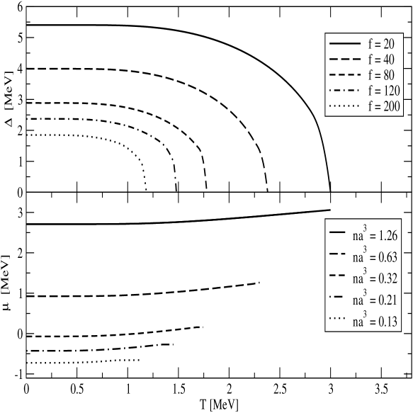
Figure 1: Dependence of the pairing gap (upper panel) and the chemical potential (lower panel) on temperature for fixed values of the ratio $f=n_{0}/n$, where $n$ is the baryon density and $n_{0}=0.16$ fm^-3 is the saturation density of symmetrical nuclear matter. Values of the diluteness parameter $na^{3}$ assume a scattering length $a=5.4$ fm.

The top panel of Fig. 1 shows the dependence of the gap function on temperature for several densities $n$, given in terms of the ratio $f=n_{0}/n$, where $n_{0}=0.16$ fm^-3 is the saturation density of symmetrical nuclear matter. The bottom panel shows the associated chemical potentials $\mu$ computed self-consistently from Eq. (22). The low- and high-temperature asymptotics of the gap function are well described by the BCS relations $\Delta(T\to 0)=\Delta(0)-[2\pi\alpha\Delta(0)T]^{1/2}\,{\rm exp}(-\Delta(0)/T)$ and $\Delta(T\to T_{c2})=3.06\beta[T_{c2}(T_{c2}-T)]^{1/2}$, respectively, where $T_{c2}$ is the critical temperature of the phase transition. However, the BCS weak-coupling values $\alpha=1=\beta$ must be replaced with $\alpha\sim 0.2$ and $\beta\sim 0.9$. As a consequence, the ratio of the gap at zero temperature to the critical temperature deviates from the familiar BCS result $\Delta(0)/T_{c2}=1.76$. The deviations from BCS theory are understandable in that (i) the system is in the strong-coupling regime, and (ii) the pairing is in a spin-triplet state rather than spin-singlet [i.e., $D(p)\neq\Delta(p)]$.

One measure of coupling strength is the ratio $\Delta(0)/|\mu|$ of the zero-temperature energy gap to the magnitude of the chemical potential. It is seen from Fig. 1 that the strong-coupling regime is realized for $f\geq 40$ (i.e. $\Delta\gg\mu$). At $f=20$ the system is in a transitional regime ($\Delta\sim\mu$). Another measure of coupling is the diluteness parameter $n|a|^{3}$, where $a$ is the scattering length. In agreement with the above criterion, the matter is in the dilute (or strong-coupling) regime for $f\geq 40$, since this corresponds to $na^{3}=0.63<1$ when $a$ is taken as the triplet neutron-proton scattering length, 5.4 fm. A signature of the crossover from weak to strong coupling is the change of the sign of the chemical potential, which occurs for $f\approx 80$ (Fig. 1), slightly below the crossover density between weak- and strong-coupling regimes.

In the limit of vanishing density, $f\to\infty$, the value of the chemical potential at $T=0$ tends to $\mu(\infty)=-1.1$ MeV, which is half the binding energy of the deuteron in free space SD_ASYMMETRIC2 . Indeed, in this limit the gap equation reduces to the Schrödinger equation for the two-body bound state, with the chemical potential assuming the role of the energy eigenvalue BCS_BEC1 . Thus, the BCS condensate of Cooper pairs in the $3S1$ state evolves into a Bose-Einstein condensate of deuterons as the system crosses over from the weak- to the strong-coupling regime. The crossover is smooth, taking place without change of symmetry of the many-body wave function.

II.4 Two-body bound states

Next let us consider temperatures above the critical temperature of pair condensation. The two-body $T$-matrix that sums up the particle-particle ladders for a system interacting with the potential $V$ obeys the operator equation

$${\bm{T}}={\bm{V}}+{\bm{V}}{\bm{G}_{0}}{\bm{T}}={\bm{V}}+{\bm{T}}{\bm{G}_{0}}{\bm{V}}.$$ (26)

Since the potential is time-local, the $T$-matrix depends on two time arguments (instead of four in general), and its transformation properties are identical to those of the two-point correlation functions discussed above. The four-momenta $P=(E,\bm{P})$ and $p=(\epsilon,\bm{p})$ in the center-of-mass system are related to their counterparts $k_{1,2}=(\omega_{1,2},\bm{k}_{1,2})$ in the laboratory system through $P=k_{1}+k_{2}$ and $p=(k_{1}-k_{2})/2$.

In the momentum representation, Eq. (26) takes the form

$$T^{R}(\bm{p},\bm{p}^{\prime};\bm{P},E) = V(\bm{p},\bm{p}^{\prime})+\int\frac{d\bm{p}^{\prime\prime}}{(2\pi)^{3}}V(\bm{p},\bm{p}^{\prime\prime})$$ (27)

$$\times G_{0}^{R}(\bm{p}^{\prime\prime},\bm{P},E)T^{R}(\bm{p}^{\prime\prime},\bm{p}^{\prime};\bm{P},E)$$

for the retarded component of the $T$-matrix. The relevant two-body Green’s function is

$$G_{0}^{R}(\bm{k}_{1},\bm{k}_{2},E) = \int_{\omega_{1}\omega_{2}}\!\!\frac{G^{>}(k_{1})G^{>}(k_{2})-G^{<}(k_{1})G^{<}(k_{2})}{E-\omega_{1}-\omega_{2}+i\eta}$$ (28)

$$= \frac{Q_{2}(\bm{k}_{1},\bm{k}_{2})}{E-\epsilon(\bm{k}_{1})-\epsilon(\bm{k}_{2})+i\eta},$$

where the second relation follows in the quasiparticle approximation and we introduce the abbreviation $\int_{\omega}=\int d\omega/(2\pi)$. The two-body phase-space occupation factor $Q_{2}(\bm{k}_{1},\bm{k}_{2})=1-f(\bm{k}_{1})-f(\bm{k}_{2})$, operating in intermediate states, allows for propagation of particles and holes, thereby incorporating time-reversal invariance. The two-body $T^{R}$-matrix has a pole at the energy corresponding to the two-body bound state. If $Q_{2}=1$, the pole is exactly at the binding energy of the deuteron; otherwise the pole on the real energy axis determines the binding energy of a dimer in the background medium of finite density and temperature. Numerical solutions of Eq. (27) will be considered after treating the problem of trimer binding in the next section.

III Three-body bound states

For completeness, we first recapitulate the three-body equations SEDRAKIAN_ROEPKE that are used in Subsec. III.2 at finite density and temperature to obtain an integral equation for the wave function of the three-body bound states. Readers more concerned with the numerical results can go immediately to Subsec. III.2.

III.1 Formalism

A fermionic system supports three-body bound states when there exists a non-trivial negative energy solution to the homogeneous counterpart of the three-body equation

$${\cal T}={\cal V}+{\cal V}\,{\cal G}\,{\cal V}={\cal V}+{\cal V}\,{\cal G}_{0}\,{\cal T},$$ (29)

for the three-body ${\cal T}$-matrix, where ${\cal V}$ is the three-body interaction and ${\cal G}$ and ${\cal G}_{0}$ are the full and free three-body Green’s functions. For compactness Eq. (29) is written in the operator form. If we assume that the particles of the system interact via two-body forces, the three-body interaction between any three particles (123) reduces to a sum of pairwise interactions ${\cal V}={\cal V}_{12}+{\cal V}_{23}+{\cal V}_{13}$, where ${\cal V}_{ij}$ is the interaction potential between particles $i$ and $j$. The kernel of Eq. (29) is not square integrable, since the pair potentials introduce momentum-conserving delta-functions for the spectator non-interacting particle. As a consequence, the iteration series contain singular terms (e.g. of type ${\cal V}_{ij}{\cal G}_{0}{\cal V}_{ij}$ to the lowest order in the interaction). However, a complete resummation of the ladder series in any particular two-body channel $ij$ takes care of this problem.

We decompose the three-body scattering matrix as ${\cal T}={\cal T}^{(1)}+{\cal T}^{(2)}+{\cal T}^{(3)}$, where

$${\cal T}^{(k)}={\cal V}_{ij}+{\cal V}_{ij}{\cal G}_{0}{\cal T}$$ (30)

and $ijk=123,\,231,\,312.$ The channel $ij$ transition operators ${\cal T}_{ij}$ resum the successive iterations with the driving term ${\cal V}_{ij}$, according to

$${\cal T}_{ij}={\cal V}_{ij}+{\cal V}_{ij}{\cal G}_{0}{\cal T}_{ij}.$$ (31)

Eqs. (30) and (31) are combined to eliminate the two-body interactions in favor of the channel matrices and arrive at a systemFADDEEV ; BETHE

$${\cal T}^{(k)} = {\cal T}_{ij}+{\cal T}_{ij}{\cal G}_{0}\left({\cal T}^{(i)}+{\cal T}^{(j)}\right)$$ (32)

$$= {\cal T}_{ij}+\left({\cal T}^{(i)}+{\cal T}^{(j)}\right){\cal G}_{0}{\cal T}_{ij}.$$

of three coupled, nonsingular integral equations of Fredholm type II. The ${\cal T}_{ij}$-matrices are essentially the two-body scattering amplitudes, embedded in the Hilbert space of three-body states. Analysis of the bound-state problem is based on the homogeneous version of Eq. (30).

The medium modifications encoded in the three-body propagator ${\cal G}_{0}$ become apparent when it is written in the momentum representation SEDRAKIAN_ROEPKE ,

$${\cal G}_{0}(\bm{k}_{1},\bm{k}_{2},\bm{k}_{3},\Omega) = \int_{\omega_{1},\omega_{2},\omega_{3}}\!\Bigl{[}G^{>}(k_{1})G^{>}(k_{2})G^{>}(k_{3})$$ (33)

$$-G^{<}(k_{1})G^{<}(k_{2})G^{<}(k_{3})\Bigr{]}$$

$$=\frac{Q_{3}(\bm{k}_{1},\bm{k}_{2},\bm{k}_{3})}{\Omega-\epsilon(\bm{k}_{1})-\epsilon(\bm{k}_{2})-\epsilon(\bm{k}_{3})+i\eta},$$

where the $k_{i}=(\omega_{i},\bm{k}_{i})$ are the particle four-momenta and

$$Q_{3}(\bm{k}_{1},\bm{k}_{2},\bm{k}_{3}) = [1-f(\bm{k}_{1})][1-f(\bm{k}_{2})][1-f(\bm{k}_{3})]$$ (34)

$$- f(\bm{k}_{1})f(\bm{k}_{2})f(\bm{k}_{3})$$

is the intermediate-state phase-space occupation factor for three-particle propagation. In the second line of Eq. (33), the intermediate-state propagation is constrained to the mass shell within the quasiparticle approximation. The momentum space for the three-body problem is spanned by the Jacobi four-momenta $K=k_{i}+k_{j}+k_{k}$, $p_{ij}=(k_{i}-k_{j})/2$, an $q_{k}=(k_{i}+k_{j})/3-2k_{k}/3$. The expressions for particle momenta in terms of Jacobi coordinates, namely $k_{1}={K}/{3}+p_{13}+{q_{2}}/{2}$, $k_{2}={K}/{3}-p_{13}+{q_{2}}/{2}$, and $k_{3}={K}/{3}-{q_{2}}$, are to be substituted into Eq. (33).

To obtain the bound-state energy, it is convenient to work with the wave function components $\psi^{(i)}$ rather than the ${\cal T}^{(i)}$ matrices. The total wave function of the three-body state is given by the sum

$$\Psi=\psi^{(1)}+\psi^{(2)}+\psi^{(3)}$$ (35)

of its three components, which, in analogy to Eq. (30), obey the homogeneous equations

$$\psi^{(k)}={\cal G}_{0}T_{ij}(\psi^{(i)}+\psi^{(j)}).$$ (36)

For identical particles these equations reduce to a single equation

$$\psi^{(1)}={\cal G}_{0}T_{23}(P_{12}P_{23}+P_{13}P_{23})\psi^{(1)}={\cal G}_{0}T_{23}P\psi^{(1)},$$ (37)

where $P=P_{12}P_{23}+P_{13}P_{23}$ and $P_{ij}$ permutes the indices i and j. The total wave function is obtained as $\Psi=(1+P)\psi^{(1)}$.

III.2 Solving for bound states

Eq. (37) can be reduced further to an integral equation in two continuous variables by working with states diagonal in the angular-momentum basis,

$$|pq\alpha\rangle_{i}\equiv|pq(l\lambda)LM(s\frac{1}{2})SM_{S}\rangle_{i},$$ (38)

where $p$ and $q$ are the magnitudes of the relative momenta of the pair $\{kj\}$ (indicated by the complementary index $i$), $l$ and $\lambda$ are their associated relative angular-momentum quantum numbers, $s$ is their total spin, and $LMSM_{S}$ are the orbital and spin quantum numbers of the three-body system. The channel $\cal T$-matrix of the pair $\{kj\}$ in this basis takes the form

$$\langle pq\alpha|{\cal T}_{kj}|p^{\prime}q^{\prime}\alpha^{\prime}\rangle=\delta_{\alpha,\alpha^{\prime}}\frac{\delta(q-q^{\prime})}{q^{2}}T\left(p,p^{\prime},E-q^{2}/2m\right),$$

while, with $\omega\equiv E-q^{2}/2m$, the two-body $T$-matrix in the two-particle space has the structure

$$\langle plm_{l}sm_{s}|T(\omega)|p^{\prime}l^{\prime}m^{\prime}_{l}s^{\prime}m^{\prime}_{s}\rangle=\delta_{ll^{\prime}}\delta_{m_{l}m^{\prime}_{l}}\delta_{ss^{\prime}}\delta_{m_{s}m_{s}^{\prime}}\langle p|T(\omega)|p^{\prime}\rangle.$$

The states are normalized such that $\langle plm_{l}sm_{s}|p^{\prime}l^{\prime}m_{l}^{\prime}s^{\prime}m_{s}^{\prime}\rangle=p^{-2}\delta(p-p^{\prime})\delta_{ll^{\prime}}\delta_{m_{l}m_{l}^{\prime}}\delta_{ss^{\prime}}\delta_{m_{s}m_{s}^{\prime}}.$ The two-body $T$-matrix is governed by Eq. (27), rewritten as

$$\langle p|T(\omega)|p^{\prime}\rangle=\langle p|V|p^{\prime}\rangle+\int\!\!\frac{dp^{\prime\prime}{p^{\prime}}^{\prime 2}}{4\pi^{2}}\langle p^{\prime}|V|p^{\prime\prime}\rangle\frac{Q_{2}(p,q)}{\omega-\epsilon_{+}(q,p)-\epsilon_{-}(q,p)+i\eta}\langle p^{\prime\prime}|T(\omega)|p^{\prime}\rangle,$$ (41)

where $Q_{2}(q,p)=\langle 1-f(\bm{q}/2+\bm{p})-f(\bm{q}/2+\bm{p})\rangle$ and $\epsilon_{\pm}(q,p)=\langle\epsilon(\bm{q}/2\pm\bm{p})\rangle$ are averaged over the angle between the vectors $\bm{q}$ and $\bm{p}$. The three-body propagator in the $|pq\alpha\rangle_{i}$ basis has the form

$$\langle pq\alpha|{\cal G}_{0}(\Omega)|p^{\prime}q^{\prime}\alpha^{\prime}\rangle=\delta_{\alpha\alpha^{\prime}}\frac{\delta(p-p^{\prime})}{p^{2}}\frac{\delta(q-q^{\prime})}{q^{2}}\frac{Q_{3}(q,p)}{\Omega-\epsilon_{+}(q,p)-\epsilon_{-}(q,p)-\epsilon(-q)},$$ (42)

with $Q_{3}(q,p)$ given by the angle average of Eq. (34). Here the propagator is assumed to be independent of the momentum of the three-body system with respect to the background ($\bm{K}=0$). Finally, the required expression for the permutation operator $P$ in the chosen basis is

$$\langle pq\alpha|P|p^{\prime}q^{\prime}\alpha^{\prime}\rangle=\int_{-1}^{1}dx\frac{\delta(\pi_{1}-p)}{p^{l+2}}\frac{\delta(\pi_{2}-p^{\prime})}{(p^{\prime})^{l^{\prime}+2}}{H}_{\alpha\alpha^{\prime}}(q,q^{\prime}x).$$ (43)

In this expression, $\pi_{1}^{2}=q^{\prime 2}+q^{2}/4+qq^{\prime}x$ and $\pi_{2}^{2}=q^{2}+q^{\prime 2}/4+qq^{\prime}x$, where $x$ is the angle formed by $\bm{q}$ and $\bm{q}^{\prime}$, while

$${H}_{\alpha\alpha}(q,\bar{q}^{\prime},x)=\sum_{n=0}^{\infty}P_{n}(x)\sum_{l_{1}+l_{2}=l}\sum_{l^{\prime}_{1}+l^{\prime}_{2}=l^{\prime}}q^{l_{2}+l^{\prime}_{2}}(q^{\prime})^{l_{2}+l^{\prime}_{2}}h_{\alpha\alpha^{\prime}}^{nl_{1}l_{1}^{\prime}l_{2}l^{\prime}_{2}}.$$ (44)

In turn, $P_{n}(x)$ denotes the Legendre polynomial, and the coefficients $h_{\alpha\alpha^{\prime}}^{nl_{1}l_{1}^{\prime}l_{2}l^{\prime}_{2}}$ are combinations of $3j$ and $6j$ symbols GLOECKLE . The resulting integral equations can be solved by iteration TJON .

Compared to the free-space problem, the three-body equations in the background medium now include two- and three-body propagators that account for (i) the suppression of the phase-space available for scattering in intermediate two-body states, encoded in the functions $Q_{2}=1-f(k_{i})-f(k_{j})$, (ii) the phase-space occupation for the intermediate three-body states, encoded in the function $Q_{3}=[1-f(k_{i})][1-f(k_{j})][1-f(k_{k})]-f(k_{i})f(k_{j})f(k_{k})$, (iii) renormalization of the single particle energies $\epsilon(p)$ (although the numerical calculations to be reported are carried out with the free single-particle spectrum). For small temperatures the quantum degeneracy is large and the first two factors significantly reduce the binding energy of a three-body bound state; at a critical temperature $T_{c3}$ corresponding to $E_{t}(\beta)=0$, the bound state enters the continuum.

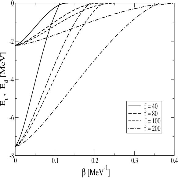
Figure 2: Dependence of the two-body ($E_{d}$) and three-body ($E_{t}$) binding energies on inverse temperature, for fixed values of the ratio $f=n_{0}/n$, where $n$ is the baryon density and $n_{0}=0.16$ fm^-3 is saturation density of nuclear matter. For asymptotically large temperature, $E_{d}(\infty)=-2.23$ MeV and $E_{t}(\infty)=-7.53$ MeV. The ratio $E_{t}(\beta)/E_{d}(\beta)$ is a universal constant independent of temperature.

Figure 3: Wave function of the three-body bound state as a function of the Jacobi momenta $p$ and $q$ defined in the text, for $f=n_{0}/n=60$ and temperatures (top to bottom) $T=60$, 10, and 6.6 MeV.

This feature is illustrated in Fig. 2, which shows the temperature dependence of the two- and three-body bound-state energies in dilute nuclear matter for several values of the density of the environment. The effect of temperature on the two-body bound state is due to the $Q_{2}$ factor only. In analogy to the behavior of the in-medium three-body bound state, the binding energy of the two-body bound state enters the continuum at a critical temperature $T_{c2}$, corresponding to the condition $E_{d}(\beta)=0$.

The solutions obtained exhibit a remarkable feature: the ratio $\eta=E_{t}(\beta)/E_{d}(\beta)$ is a constant independent of temperature. For the chosen potentials, the asymptotic free-space values of the binding energies are $E_{t}(0)=-7.53$ MeV and $E_{d}(0)=-2.23$ MeV; hence $\eta=3.38$. An alternative definition of the critical temperature for trimer extinction is $E_{t}(\beta_{3c}^{\prime})=E_{d}(\beta)$. This definition takes into account the break-up channel $t\to d+n$ of the three-body bound state into the two-body bound state $d$ and a nucleon $n$. The difference between the two definitions is insignificant, because of the property $\eta(\beta)=$ Const. The binding energies of the two and three-body bound states, as well as their ratio, depend on the choice of the interaction. The universality pointed out above applies only to the temperature dependence of these quantities. It should be tested for other interactions in the future.

Fig. 3 depicts the normalized three-body bound-state wave function for three representative temperatures, as a function of the Jacobi momenta $p$ and $q$. (The temperature decreases from top to bottom). As the temperature drops, the wave function becomes increasingly localized around the origin in momentum space. Correspondingly, the radius of the bound state increases in $r$-space, eventually tending to infinity at the transition. The wave-function oscillates near the transition temperature (bottom panel of Fig. 3). This oscillatory behavior is a precursor of the transition to the continuum, which in the absence of a trimer-trimer interaction is characterized by plane-wave states.

IV Summary and outlook

The complexity of the phase diagram of low-density, finite-temperature nuclear matter is twofold: (i) The system supports liquid-gas and superfluid phase transitions. Thus, depending on the temperature and density, nuclear matter can be in the gaseous, fluid, or superfluid state. These features are generic to systems of fermions interacting with “van der Waals type” forces that are repulsive at short range and attractive at large separations. (ii) The attractive component of these forces leads to clustering. The clustering pattern is non-universal and depends on the form of the attractive force in a particular system.

Fig. 4 combines results from Secs. III and IV in plots of the critical temperatures for the superfluid phase transition ($T_{c2}$) and for extinction of three-body bound-states ($T_{c3}$), as functions of density. The phase diagram divides into several distinct regions: (A) The low-density, high-temperature domain is populated by trimers, which enter the continuum when the critical line $T_{c3}(n)$ is crossed from above. (B) The low-temperature and low-density domain ($na^{3}\ll 1$ , $f<40$) contains a Bose condensate of tightly-bound deuterons. (C) The low-temperature, high-density domain features a BCS condensate of weakly-bound Cooper pairs ($na^{3}\gg 1$). (D) The domain between the two critical lines contains nucleonic liquid. The phases C and D are characterized by broken symmetry associated with the $\langle\psi\psi\rangle$ condensate. The transition C$\to$B does not involve symmetry changes and is a smooth crossover from the BCS to BE condensate. The transitions B$\to$D and C$\to$D are second-order phase transitions related to the vanishing of the condensate along the line $T_{c2}(n)$. The transition A$\to$D can be characterized by an order parameter given by the fraction of trimers, which goes to zero at the transition. This transition appears to be of second order; however, a study of thermodynamics of the transition will be needed for confirmation.

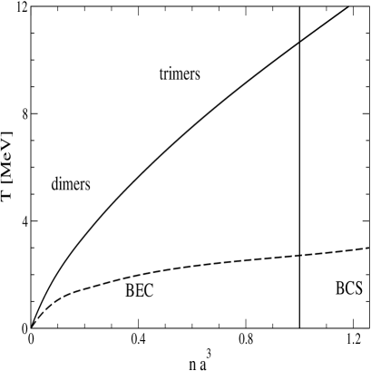
Figure 4: Dependence of the critical temperature of extinction of three-body bound-states on density (solid line). Trimers exist above this critical line. The dependence of the critical temperature of the superfluid phase transition is shown by the dashed line. The condensate is a weakly-coupled BCS superfluid far to the right of the vertical line and is a Bose-Einstein condensate of tightly-bound pairs far to the left, with a smooth crossover transition in between.

To summarize, we have studied the temperature-density phase diagram of dilute isospin-symmetric nuclear matter, which features an isospin-singlet, spin-triplet pair condensate at low temperature and a gas of trimers (three-body bound-states) at high temperature. Solving self-consistently for the gap function and the chemical potential, we have quantified the behavior of the system in the density-temperature domain where the Cooper condensate crosses over to a BEC condensate of tightly-bound deuterons. A modified iterative procedure for solution of the gap equation with a “running” cutoff has been designed and implemented for this purpose. The method is found to be effective in treating the strong repulsive core of the potential. Solution of the three-body integral equations for bound states in the background medium furnishes us with density and temperature-dependent binding energies of trimers in dilute nuclear matter. Numerically, we find that the ratio of the temperature-dependent binding energies of dimers and trimers is independent of the temperature and density and can be determined from its value in free space. For large degeneracies, the binding energy of trimers is small and vanishes at a critical temperature $T_{c3}$ which is larger than the critical temperature of superfluid phase transition $T_{c2}$. These critical lines $T_{c3}(n)$ and $T_{c2}(n)$ separate the phase diagram into distinct regions. At the high-temperature/low-density end the system is populated by trimers, whereas in the low-temperature/high-density regime the system supports a condensate of neutron-proton Cooper pairs, which crosses over to a Bose-Einstein condensate of deuterons as the density decreases.

We have omitted a number of correlation effects in our discussion. (i) The momentum and energy dependent self-energies renormalize the spectrum of quasiparticles in nuclear matter. While these renormalizations are important at densities comparable to the nuclear saturation density, it is likely that their influence on the physics at much smaller densities ($f\leq 40$) is minor. (ii) It is known that the screening of interactions, associated with long-wave length density and spin fluctuations, are important for dilute fermions; e. g. they change the value of the pairing gap by a factor of 0.45 S10_PAIRING ; Gorkov61 ; Papen99 ; Pethick00 . A task for the future is to incorporate the screening of interactions in the bound state calculations discussed above.

Clearly, the true phase diagram of dilute and finite-temperature nuclear matter is richer than that derived from the present study. Modifications are likely to originate from clusters with $A=4$ and their Bose-Einstein condensation ALPHA_CONDENSATION . Still, we expect that although the phase diagram shown in Fig. 4 has been obtained for a particular form of the two-body interaction, its qualitative features should be universal for saturating systems of attractive fermions that possess two- and three-body bound states in free space.

References

- (1) B. DeMarco and D. S. Jin, Science 285, 1703 (1999); K. M. O’Hara, S. L. Hemmer, M. E. Gehm, S. R. Granade, and J. E. Thomas, Science 13, 2179 (2002); C. A. Regal, C. Ticknor, J. L. Bohn, and D. S. Jin, Phys. Rev. Lett. 90, 053201 (2003); K. E. Strecker, G. B. Partridge, and R. G. Hulet, Phys. Rev. Lett. 91, 080406 (2003); M. W. Zwierlein, C. A. Stan, C. H. Schunck, S. M. F. Raupach, S. Gupta, Z. Hadzibabic, and W. Ketterle, Phys. Rev. Lett. 91, 250401 (2003); M. Greiner, C. A. Regal, and D. S. Jin, Nature (London) 426, 537 (2003); C. A. Regal, M. Greiner, and D. S. Jin, Phys. Rev. Lett. 92, 040403 (2004);
- (2) C. Chin, M. Bartenstein, A. Altmeyer, S. Riedl, S. Jochim, J. Hecker Denschlag and R. Grimm, Science 305, 1128 (2004); T. Bourdel, L. Khaykovich, J. Cubizolles, J. Zhang, F. Chevy, M. Teichmann, L. Tarruell, S. J. J. M. F. Kokkelmans and C. Salomon Phys. Rev. Lett. 93, 050401 (2004); G. B. Partridge, K. E. Strecker, R. I. Kamar, M. W. Jack, and R. G. Hulet, Phys. Rev. Lett. 95, 020404 (2005).
- (3) G. Ortiz and J. Dukelsky, Phys. Rev. A 72, 043611 (2005); Y. Ohashi and A. Griffin, eprint cond-mat/0508213; Q.-J. Chen, J. Stajic and K. Levin, eprint cond-mat/0508603; M. W. J. Romans and H. T. C. Stoof, eprint cond-mat/0506282; D. E. Sheehy and L. Radzihovsky, eprint cond-mat/0508430; D. T. Son and M. A. Stephanov, eprint cond-mat/0507586; Kun Yang, Phys. Rev. Lett. 95, 218903 (2005); Kun Yang, eprint cond-mat/0508484; A. Sedrakian, J. Mur-Petit, A. Polls, H. Müther, Phys.Rev. A 72, 013613 (2005); C. Honerkamp and W. Hofstetter, Phys. Rev. B 70, 094521 (2004).
- (4) J. M. Lattimer and D. Swesty, Nucl. Phys. A535, 331 (2001); H. Shen, H. Toki, K.Oyamatsu and K. Sumiyoshi, Prog. Theor. Phys. 100, 1013 (1998); Nucl. Phys. A637, 435 (1998).
- (5) D. J. Dean and M. Hjorth-Jensen, Rev. Mod. Phys. 75, 607 (2003).
- (6) The work in this field is reviewed by K. Rajagopal and F. Wilczek, ”At the Frontier of Particle Physics / Handbook of QCD”, M. Shifman, ed., (World Scientific, 2001) [hep-ph/0011333]; M. Alford, Prog. Theor. Phys. Suppl. 153, 1 (2004); D. Rischke, Prog. Part. Nucl. Phys. 52, 197 (2004); T. Schaefer, hep-ph/0509068.
- (7) M. V. Zverev, J. W. Clark, V. A. Khodel Nucl. Phys. A720, 20 (2003); J. W. Clark, V. A. Khodel, M. V. Zverev, nucl-th/0203046; V. A. Khodel, J. W. Clark, M. V. Zverev, Phys. Rev. Lett. 87 031103 (2001); V. V. Khodel, V. A. Khodel, J. W. Clark, Nucl. Phys. A679, 827 (2001); V. A. Khodel, J. W. Clark, M. Takano, and M. V. Zverev, Phys. Rev. Lett. 93, 151101 (2004)
- (8) M. Baldo, O. Elgaroy, L. Engvik, M. Hjorth-Jensen, and H.-J. Schulze, Phys. Rev. C 58, 1921 (1998).
- (9) T. Takatsuka and R. Tamagaki, Prog. Theor. Phys. Suppl. 112,27 (1993). A. Sedrakian, G. Röpke and T. Alm, Nucl. Phys. 594, 355, (1995). T. Alm, G. Röpke, A. Sedrakian and F. Weber, Nucl. Phys. A604, 491 (1996).
- (10) T. Alm, G. Röpke, and M. Schmidt, Z. Phys. A337, 355 (1990); B. E. Vonderfecht, C. C. Gearhart, W. H. Dickhoff, A. Polls, and A. Ramos, Phys. Lett. B253, 1 (1991); M. Baldo, I. Bombaci and U. Lombardo, Phys. Lett. B283, 8 (1992); M. Baldo, U. Lombardo, H.-J. Schulze, and Z. Wei Phys. Rev. C 66, 054304 (2002); C. Shen, U. Lombardo, and P. Schuck Phys. Rev. C 71, 054301 (2005); H. Müther and W. H. Dickhoff, nucl-th/0508035.
- (11) A. J. Leggett, in Modern Trends in the Theory of Condensed Matter (Springer, Berlin, 1980), p.13; J. Phys. (Paris) 41, C7-19 (1980); L. V. Keldysh and Yu. V. Kopaev, Sov. Phys. Solid State 6, 2219 (1965); L. V. Keldysh and A. N. Kozlov, Sov. Phys. JETP 27, 521 (1968); P. Nozières and S. Schmitt-Rink, J. Low Temp. Phys. 59, 195 (1985).
- (12) T. Alm, B. L. Friman, G. Röpke, and H. Schulz, Nucl. Phys. A551, 45 (1993); M. Baldo, U. Lombardo, and P. Schuck, Phys. Rev. C52, 975 (1995).
- (13) A. Sedrakian, T. Alm, and U. Lombardo, Phys. Rev. C55, R582 (1997); A. Sedrakian and U. Lombardo, Phys. Rev. Lett. 84, 602 (2000).
- (14) U. Lombardo, P. Nozières, P. Schuck, H.-J. Schulze and A. Sedrakian, Phys. Rev. C64, 064314 (2001).
- (15) The extensive literature on pairing in the channel is review in ref. RIA and by U. Lombardo and H.-J. Schulze, Lecture Notes in Physics, vol 578, pg 30 (Springer, Berlin, 2001).
- (16) A. L. Goodman, Phys. Rev. C60, 014311 (1999), and references therein; B. K.-L. Kratz, J.-P. Bitouzet, F.-K. Thielmann, and B. Pfeiffer, Astrophys. J. 403, 216 (1993). B. Chen, J. Dobaczewski, K.-L. Kratz, K. Langanke, B. Pfeiffer, F.-K. Thielmann, and P. Vogel, Phys. Lett. B355, 37 (1995); G. Röpke, A. Schnell, P. Schuck, and U. Lombardo, Phys. Rev. C61, 024306 (2000).
- (17) G. V. Skorniakov and K. A. Ter-Martirosian, Sov. Phys. JETP 4, 648 (1957).
- (18) L. D. Faddeev, Sov. Phys. JETP 12, 1014 (1961).
- (19) H. A. Bethe, Phys. Rev. 138, B804 (1965); H. A. Bethe, Phys. Rev. 158, 941-947 (1967); R. Rajaraman, Phys. Rev. 155, 1105 (1967).
- (20) B. D. Day, Rev. Mod. Phys. 39, 719 (1967); H. Q. Song, M. Baldo, G. Giansiracusa, U. Lombardo, Phys. Rev. Lett. 81, 1584 (1998); M. Baldo, A. Fiasconaro, H. Q. Song, G. Giansiracusa, U. Lombardo, Phys. Rev. C 65, 017303 (2001); R. Sartor, Phys. Rev. C 68, 057301 (2003).
- (21) J. Dukelsky and P. Schuck, Nucl. Phys. A512, 466 (1990); see also P. Schuck, F. Villars, and P. Ring, Nucl. Phys. A208, 302 (1973).
- (22) A. Sedrakian and G. Röpke, Ann. Phys. (NY) 266, 524 (1998).
- (23) A. N. Kvinikhidze and B. Blankleider, Phys.Rev. C 72, 054001 (2005).
- (24) O. Alt, P. Grassberger and W. Sandhas, Nucl. Phys. B2, 167 (1967).
- (25) M. Beyer et al, Phys. Lett. B 376, 7 (1996); M. Beyer, W. Schadow, C. Kuhrts, G. Röpke, Phys. Rev. C 60, 034004 (1999).
- (26) R. A. Malfliet and J. A. Tjon, Nucl. Phys. A127, 161 (1969).
- (27) J. W. Serene and D. Reiner, Phys. Rep. 101, 221 (1983).
- (28) E. Krotscheck, Z. Phys. 251, 135 (1972).
- (29) V. V. Khodel, V. A. Khodel and J. W. Clark, Nucl. Phys. A598, 390 (1996).
- (30) O. Elgaroy, L. Engvik, M. Hjorth-Jensen and E. Osnes, Nucl. Phys. A604, 466 (1996).
- (31) W. Glöckle, The Quanum Mechanical Few-Body Problem (Springer, Berlin 1983).
- (32) L. P. Gor’kov amd T. K. Melik-Barkhudarov, Sov. Phys. JETP 13, 1018 (1961).
- (33) T. Papenbrock and G. F. Bertsch, Phys. Rev. C 59, 2052 (1999).
- (34) H. Heiselberg, C. J. Pethick, H. Smith and L. Viverit, Phys. Rev. Lett. 85, 2418 (2000).
- (35) M. T. Johnson and J. W. Clark, Kinam 3, 3 (1980); G. Röpke, A. Schnell, P. Schuck and P. Nozières, Phys. Rev. Lett. 80, 3177-3180 (1998); A. Sedrakian, H. Müther and P. Schuck, Nucl. Phys. A 766, 97 (2006).