Manifestation of the cyclo-toroid nuclear moment in anomalous conversion and Lamb shift

Abstract

We offer the hypothesis that atomic nuclei, nucleons, and atoms possess a new type of electromagnetic moment, that we call a “cyclo-toroid moment”. In nuclei, this moment arises when the toroid dipole (anapole) moments are arrayed in the form of a ring, or, equivalently, when the magnetic moments of the nucleons are arranged in the form of rings which, in turn, constitute the surface of a torus. We establish theoretically that the cyclo-toroid moment plays a role in the processes of the atomic shell–nucleus interaction. The existence of this moment would explain known anomalies in the internal conversion coefficients for $M1$ transitions in nuclei. We show also that the static cyclo-toroid nuclear moment interacts locally inside the nucleus with the vortex part of the atomic electron currents and this leads to an energy shift in atomic $s_{1/2}$ states. For the hydrogen atom the value of this shift may be comparable in order of magnitude to the present accuracy of measurements of the Lamb shift for the $1s_{1/2}$ level.

I 1. Introduction

The existence of anapole moment was theoretically predicted by Zel’dovich fifty years ago Zel’dovich (1957). The anapole moment arises in the system where currents or magnetic moments of particles create a ring-like closed distribution of magnetic field lines. A classic example of such distribution can be a magnetic field inside the toroidal solenoid over the surface of which poloidal currents flow. A less trivial example is an atomic nucleus in which spins of nucleons compose a ring with forming the corresponding configuration of the magnetic field. The great interest to the anapole is related to fundamental investigations on the parity nonconservation in atomic-nuclear interactions Bouchiat and Bouchiat (1997); Flambaum and Khriplovich (1980). In 1997 the anapole moment of the nucleus ¹³³Cs was discovered just in the experiment on parity nonconservation in the atomic transition $6s\rightarrow 7s$ of Cs Wood et al. (1997).

Now the anapole is regarded as a dipole moment of the fundamental family of toroid moments Dubovik and Cheshkov (1974); Dubovik and Tugushev (1990) which naturally arise when currents on a torus surface are described. Toroid moments are now used in problems of current parametrization and of radiation theory Dubovik and Cheshkov (1974), in investigations of topological effects in quantum mechanics (the Aharonov-Bohm effect Afanasiev et al. (1996)), in elementary particle physics (toroid dipole momentum of neutrino Bukina et al. (1998) and $NN$-scattering Haxton et al. (2001) for example), in the theory of anomalous internal conversion Listengarten et al. (1981), in atomic physics (anapole moments of atoms Lewis (1993), atomic emission in a condensed medium Tkalya (2002)), in the physics of nanostructures (carbon toroids Ceulemans et al. (1998)), in the physics of spin-ordered crystals Schmid (2001) etc. Thus the physics of toroid moments is a wide area of scientific activity ranging from elementary particles to condensed matter. At the same time, the nucleus together with the atomic shell remain one of the most suitable quantum object for probing the toroid moments. The reason is as follows. The electronic wave functions for $s_{1/2}$ and $p_{1/2}$ states have large amplitudes at the origin. As a consequence, the electronic current at such states effectively penetrates the nucleus and interacts with the toroid moment, whose magnetic field does not exceed the boundary of the nucleus. (This interaction mechanism is a direct analogy of a thought experiment offered in Ref. Zel’dovich (1957) for a toroidal solenoid immersed into the electrolyte.) Today the situation is. The static toroid dipole moment has discovered Wood et al. (1997). As regards the toroid dipole moment of transition, there are evidences Listengarten et al. (1981) that this moment results in known anomalies in the internal conversion coefficients for $E1$ transitions in nuclei Church and Weneser (1956); Green and Rose (1958); Nilsson and Rasmussen (1958); Voikhanskii and Listengarten (1959) and in the process of nuclear excitation by electron transition in the atomic shell Tkalya (1994). Thus, more detailed and precise “conversion” experiments are needed to detect the toroid dipole moment of transition.

In the present work we consider, on the example of the nucleus–atomic shell system, two new effects dealt with the toroid moments. First of all, we prove that the anomalies mentioned above for $M1$ transitions result from a “cyclo-toroid moment”. This moment arises when the toroid dipole moments are arranged in a ring. Secondary, we demonstrate a possibility of experimental investigation of the existence of the cyclo-toroid moment by measuring of the energy shift in atomic $s_{1/2}$ levels. The results obtained here would be useful for more fundamental understanding of the nontrivial distribution of the currents inside nucleus and nucleons, and for the processes of the interaction between nucleus and atomic shell.

II 2. Cyclo-toroid nuclear moment of transition

Anomalous internal conversion of $\gamma$-rays in deformed nuclei arises because of the penetration of the electron current $j_{e}(r_{e})$ into the nucleus “beneath” the nuclear current $j_{N}(r_{N})$, i.e. when the current coordinates satisfy the condition $r_{e}<r_{N}$. The reason which changes the probability of the mentioned atomic-nuclear processes originates from to the additional selection rules Nilsson and Rasmussen (1958); Voikhanskii and Listengarten (1959). Nuclear and atomic matrix elements which determine the process of de-excitation (excitation) of deformed nuclei through the atomic shell for $r_{e}<r_{N}$ are different from those for $r_{e}>r_{N}$. In some cases the additional selection rules allow the nuclear transition for $r_{e}<r_{N}$ and forbid a $\gamma$-radiative transition Voikhanskii and Listengarten (1959) with nuclear matrix element $\langle\hat{\cal{M}}_{LM}^{e/m}\rangle=\int d^{3}r_{N}\,{\bf{j}}_{N}\cdot{{\bf{A}}^{e/m^{*}}_{LM}}$ entering the probability formula for $r_{e}>r_{N}$. (Here and further ${\bf{A}}^{e/m}_{LM}$ are the standard electric/magnetic multipoles according to the gauge of $\text{div}{\bf{A}}^{e/m}_{LM}=0$ (see in Ref. Eisenberg and Greiner (1970)), and $j_{e,N}$ are current densities. We call $j_{e,N}$ “currents” for short.)

At the beginning of 80s it was found out that the real cause of the mentioned anomaly in the processes of an electric-dipole ($E1$) interaction of the nucleus with the atomic shell results from the dipole toroid moment of the transition Listengarten et al. (1981). Toroid moments are the components of electric moments Dubovik and Cheshkov (1974); Dubovik and Tugushev (1990). Moreover, the anomaly also exists in conversion magnetic-dipole ($M1$) transitions Church and Weneser (1956); Nilsson and Rasmussen (1958). Let us consider the nature of such $M1$ anomaly.

The nucleus matrix element corresponding to the anomalous part of the magnetic-dipole process of the nuclear interaction with the atomic shell is as follows Church and Weneser (1956); Voikhanskii and Listengarten (1959); Tkalya (1994)

$$\langle\hat{\cal{M}}_{1M}^{{m}^{an}}\rangle=\int d^{3}r\left(\frac{r}{r_{0}}\right)^{2}{\bf{j}}_{N}(r)\cdot{{\bf{A}}^{m^{*}}_{1M}}(\omega,r),$$ (1)

where ${\bf{A}}^{m}_{LM}(\omega,r)=j_{L}(\omega{r}){\bf{Y}}^{L}_{LM}({\bf{n}})$ Eisenberg and Greiner (1970), $\omega$ is the energy of a nuclear transition, ${\bf{n}}={\bf{r}}/r$, $j_{L}(\omega{r})$ are the spherical Bessel functions, ${\bf{Y}}^{L}_{JM}({\bf{n}})$ are the vector spherical harmonics from Ref. Varshalovich et al. (1988), $r_{0}$ is the nucleus radius. We use in this paper the system of units $\hbar=c=1$.

The operator structure of $\langle\hat{\cal{M}}_{1M}^{{m}^{an}}\rangle$ is well known. If the nuclear transition current in Eq (1) is the sum of convection and spin terms ${\bf{j}}_{N}={\bf{j}}_{N}^{c}+{\bf{j}}_{N}^{s}$, where ${\bf{j}}_{N}^{c}=-ie_{N}/2m_{N}(\varphi^{*}_{f}{\boldsymbol{\nabla}}\varphi_{i}-({\boldsymbol{\nabla}}\varphi^{*}_{f})\varphi_{i})$ and ${\bf{j}}_{N}^{s}=\text{curl}(\varphi^{*}_{f}{\hat{\boldsymbol{\mu}}}\varphi_{i})$ (we consider one-nucleon current for simplicity) then it is easy to get the following expression for the anomalous nuclear matrix element Church and Weneser (1956); Nilsson and Rasmussen (1958); Voikhanskii and Listengarten (1959)

$$\langle\hat{\cal{M}}_{1M}^{{m}^{an}}\rangle = \frac{i\sqrt{2}}{r_{0}^{2}}\int d^{3}r\big{(}{\boldsymbol{\nabla}}j_{1}(\omega{r})Y_{1M}^{*}({{\bf{n}}})\big{)}$$ (2)

$$\cdot\varphi_{f}^{*}(r)\left(\frac{e_{N}}{2m_{N}}r^{2}{\hat{\bf{L}}}-\left[{\bf{r}}({\hat{\boldsymbol{\mu}}}\cdot{\bf{r}})-2{\hat{\boldsymbol{\mu}}}r^{2}\right]\right)\varphi_{i}(r).$$

In formula (2) and in the expression for the transition current the following standard symbols were used: ${\hat{\bf{L}}}=-i[{\bf{r}}\times{\boldsymbol{\nabla}}]$ is the operator of the angular momentum, $Y_{LM}({{\bf{n}}})$ are the spherical functions Varshalovich et al. (1988), $e_{N}$, $m_{N}$ and $\varphi({\bf{r}})$ are the charge, the mass, and the wave functions of the nucleon, accordingly, ${\hat{\boldsymbol{\mu}}}$ is the operator of the magnetic moment of the nucleon: ${\hat{\boldsymbol{\mu}}}=g\mu_{N}{\hat{\boldsymbol{\sigma}}}$, where ${\hat{\boldsymbol{\sigma}}}$ are the Pauli spin matrices, $\mu_{N}$ is the nuclear magneton, $g$ is the empirical magnetic moment of the nucleon — $g=2.79$ for the proton and -1.91 for the neutron.

The spin term of the current ${\bf{j}}_{N}^{s}$ in the matrix element $\langle\hat{\cal{M}}_{1M}^{{m}^{an}}\rangle$ in Eq (1) corresponds to the operator in Eq (2) in square brackets under the integral — $\left[{\bf{r}}({\boldsymbol{\mu}}\cdot{\bf{r}})-2{\boldsymbol{\mu}}r^{2}\right]$ (here ${\boldsymbol{\mu}}$ is the density of the magnetic moment $\varphi^{*}_{f}{\hat{\boldsymbol{\mu}}}\varphi_{i}$). Let us compare this operator with a known density operator of the dipole toroid moment ${\bf{t}}=\left[{\bf{r}}({\bf{j}}\cdot{\bf{r}})-2{\bf{j}}r^{2}\right]/10$ Dubovik and Tugushev (1990), that is created by the convection current ${\bf{j}}$. Operators in square brackets have different parity and are transformed into each other by exchanging ${\bf{j}}$ and ${\boldsymbol{\mu}}$. Taking into account this fact let us introduce the new operator

$${\bf{c}}_{t}=\frac{1}{10}\left[{\bf{r}}({\boldsymbol{\mu}}\cdot{\bf{r}})-2{\boldsymbol{\mu}}r^{2}\right]$$ (3)

and find out what geometrical pattern corresponds to ${\bf{c}}_{t}$. Using the spherical functions it is easy to rewrite Eq (3) in the form:

$$\langle{{\bf{c}}_{t}}_{M}\rangle=-\frac{\sqrt{\pi}}{3}\int d^{3}rr^{2}\left({\bf{Y}}^{0}_{1M}({\bf{n}})+\frac{\sqrt{2}}{5}{\bf{Y}}^{2}_{1M}({\bf{n}})\right)\cdot{\boldsymbol{\mu}}.$$ (4)

Then let us remember that the following objects possess the toroid moment: (a) a toroidal solenoid with a current ${\bf{j}}$; (b) a ring formed by magnetic moments ${\boldsymbol{\mu}}$ Dubovik and Tugushev (1990). For case (b) the following relationship is true: ${\text{curl}}{\bf{t}}={\boldsymbol{\mu}}$, besides that $\text{div}{\bf{t}}=0$ due to Helmholtz theorem Morse and Feshbach (1953). Substituting ${\text{curl}}{\bf{t}}$ into Eq (4) instead of ${\boldsymbol{\mu}}$, we get the following relation $\langle{{\bf{c}}_{t}}_{M}\rangle=-i\sqrt{2\pi/3}\int{}d^{3}rr{\bf{Y}}^{1}_{1M}({\bf{n}})\cdot{\bf{t}}$. A sub-integral expression can be easily transformed to the vector production (see for example, in Ref. Dubovik and Tugushev (1990)). As a result, the operator ${\bf{c}}_{t}$ can be written in as follows: ${\bf{c}}_{t}=1/2[{\bf{r}}\times{\bf{t}}]$, in full accordance with similar expressions for the density of a current magnetic moment ${\boldsymbol{\mu}}_{\bf{j}}=1/2[{\bf{r}}\times{\bf{j}}]$ and for the toroid moment formed by the ring-like composed magnetic dipoles ${\bf{t}}=1/2[{\bf{r}}\times{\boldsymbol{\mu}}]$ Dubovik and Tugushev (1990).

Expression ${\bf{c}}_{t}=1/2[{\bf{r}}\times{\bf{t}}]$ results in $\text{curl}{\bf{c}}_{t}={\bf{t}}$. The geometrical image corresponding to the operator ${\bf{c}}_{t}$, is the ring-like composed dipole toroid moments ${\bf{t}}$. Therefore ${\bf{c}}_{t}$ can be called the density of cyclo-toroid moment, and $\langle{\bf{c}}_{t}\rangle$ — the cyclo-toroid moment. The properties of a cyclo-toroid are shown by the torus whose surface is formed by either ring-like composed magnetic moments ${\boldsymbol{\mu}}$, or by poloidal lines of the magnetic field (Fig. 1a). It is also possible to consider the cyclo-toroid as a sequence of toroidal solenoids all together forming again a toroidal solenoid (such objects were considered for the first time in Ref. Afanasiev et al. (1996)). In this case the equal currents flow in opposite directions on the surface of two toruses (one of them is embedded into another) as it is shown in Fig. 1b.

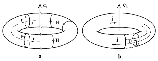
Figure 1: Cyclo-toroid.

Zel’dovich’s anapole Zel’dovich (1957) in the static case interacts with the external current $j_{ext}$ only. The energy of this interaction is $-4\pi\int{}d^{3}r\,{\bf{t}}\cdot{\bf{j}}_{ext}$. Taking also into account the equality ${\bf{t}}=\text{curl}{\bf{c}}_{t}$, we arrive straightforwardly to the Hamiltonian of the interaction of the cyclo-toroid with the external current:

$$H_{int}=4\pi\int{}d^{3}r\,{\bf{c}}_{t}\cdot\text{curl}{\bf{j}}_{ext}.$$ (5)

That is, the cyclo-toroid interacts locally (only inside the nucleus) with the vortex part of penetrating external current.

Let us determine now the role of a cyclo-toroid in the anomalous conversion. Consider the internal electron conversion from one of the $s_{1/2}$ states of an atom and show first of all that $\text{curl}{\bf{j}}\neq 0$ during the $M1$ transition of an electron to the $S_{1/2}$ state of the continuous spectrum.

We write the electron current in a common way ${\bf{j}}_{fi}=-e{\bar{\psi}}_{f}{\boldsymbol{\gamma}}\psi_{i}=-e{\psi}^{*}_{f}{\boldsymbol{\alpha}}\psi_{i}$, where ${\boldsymbol{\alpha}}=\gamma^{0}{\boldsymbol{\gamma}}$, $\gamma^{0}$ and ${\boldsymbol{\gamma}}$ are the Dirac matrixes Berestetskii et al. (1982), $e$ is the proton charge, $\psi$ are the electron wave functions. Let us write these wave functions in the form of $\psi({\bf{r}})=\left(\begin{array}[]{c}g(r){\bf\Omega}_{jlm}({\bf{n}})\\ if(r){\bf\Omega}_{jl^{\prime}m}({\bf{n}})\end{array}\right)$, where $g(r)$ and $f(r)$ are correspondingly the large and the small components of radial wave functions, ${\bf\Omega}_{jlm}({\bf n})$ are the spinor spherical harmonics Berestetskii et al. (1982). For the bound states in the atom the normalization condition is as follow: $\int_{0}^{\infty}drr^{2}(g_{i}^{2}(r)+f_{i}^{2}(r))=1$. The wave function of the final state is considered as a superposition of the plane wave and the converging spherical wave.

For the states with $j=1/2$, $l=0$ and $l^{\prime}=1$ the angular part $\psi_{m=\pm 1/2}({\bf{r}})$ is very simple, and the components of the bispinor can be written in the following way: $g(r)/\sqrt{4\pi}\left(\begin{array}[]{c}\delta_{m1/2}\\ \delta_{m-1/2}\end{array}\right)$, $if(r)/\sqrt{4\pi}\left(\begin{array}[]{c}-\cos\theta\\ -\sin\theta\exp{(i\varphi)}\end{array}\right)\delta_{m1/2}$ and $if(r)/\sqrt{4\pi}\left(\begin{array}[]{c}-\sin\theta\exp{(-i\varphi)}\\ \cos\theta\end{array}\right)\delta_{m-1/2}$. Within the spherical coordinate system the current is as follows

$$\displaystyle{}j_{r} = i\frac{-e}{4\pi}(g_{i}f_{f}-g_{f}f_{i})\delta_{m_{i}m_{f}},$$

$$j_{\theta} = \mp{i}\frac{-e}{4\pi}e^{\pm{i}\varphi}(g_{i}f_{f}+g_{f}f_{i})\delta_{m_{i}-m_{f}},$$ (6)

$$j_{\varphi} = \frac{-e}{4\pi}(g_{i}f_{f}+g_{f}f_{i})\times\left\{\begin{array}[]{l}\displaystyle{}\mp\sin\theta\delta_{m_{i}m_{f}}\\ \cos\vartheta{}e^{\pm{i}\varphi}\delta_{m_{i}-m_{f}}\end{array}\right.$$ (9)

for $m_{i}=\pm 1/2$ correspondingly. We can see that the existence of the $s_{1/2}\rightarrow{}S_{1/2}$ transition electron current itself is a totally relativistic effect. The current disappears (as it should be) when the small parts of the Dirac wave functions $f(r)$ tend to zero.

The interaction of the current with the cyclo-toroid does not occur beyond the nucleus range. Therefore, for the radial components of the $s_{1/2},S_{1/2}$ states one can use the expressions which are true for small values of arguments: $g_{i}(r)=c_{i}/a_{B}^{3/2}$, $f_{i}(r)=(c_{i}/a_{B}^{3/2})(f^{(0)}_{i}/a_{B})r$, and $g_{f}(r)=c_{f}/a_{B}$, $f_{f}(r)=(c_{f}/a_{B})(f^{(0)}_{f}/a_{B})r$, where $a_{B}$ is the Bohr radius, $c_{i,f}$ and $f^{(0)}_{i,f}$ are the coefficients of decomposition. (Here the potential inside the nucleus corresponds to the nuclear charge uniformly distributed over the spherical volume of radius $r_{0}$ Tkalya (1994).) Using the expansion, we can get from Eq (6) for ${\text{curl}}{\bf{j}}$ the following

$${\text{curl}}{\bf{j}}=\pm 2\frac{-e}{4\pi}\frac{c_{i}}{a_{B}^{3/2}}\frac{c_{f}}{a_{B}}\frac{f^{(0)}_{i}+f^{(0)}_{f}}{a_{B}}\times\left\{\begin{array}[]{l}\sqrt{2}{\bf{e}}_{\pm 1}\\ -{\bf{e}}_{0}\end{array}\right.\,,$$ (10)

where the ${\text{curl}}{\bf{j}}$ vector components are given in the polar system Varshalovich et al. (1988) and correspond to transitions $m_{i}=\pm 1/2,m_{f}=\mp 1/2$ and $m_{i}=m_{f}=\pm 1/2$ accordingly. Since $g(0)\neq 0$ and $df(r)/dr|_{r\rightarrow 0}\neq 0$ for $s_{1/2},S_{1/2}$ states, then ${\text{curl}}{\bf{j}}\neq 0$.

As an example we consider the known anomaly in the conversion $M1$ transition with the energy of $\omega_{N}=482$ keV in ¹⁸¹Ta nucleus. The experimental magnitude of the $K$ shell conversion coefficient is 3 times as great as the so-called normal theoretical magnitude Firestone (1991). The magnitude of the penetration parameter $\lambda^{(0)}=\langle\hat{\cal{M}}_{1M}^{{m}^{an}}\rangle/\langle\hat{\cal{M}}_{1M}^{m}\rangle$ equals to 150 Firestone (1991). The transition occurs between the states with quantum numbers in the Nilsson model being as follows: $J^{\pi}K[Nn_{z}\Lambda]\Sigma=5/2^{+}5/2[402]\uparrow$ and $7/2^{+}7/2[404]\downarrow$ Nilsson and Rasmussen (1958). The radiation nuclear matrix element of this transition is forbidden by asymptotic quantum numbers, while the anomalous one is allowed Nilsson and Rasmussen (1958). However, the selection rules for the operator $r^{2}{\hat{\bf{L}}}$ in Eq (2) forbid the anomaly nuclear transition in ¹⁸¹Ta Nilsson and Rasmussen (1958). Therefore we can infer that the anomaly results just from the interaction of the transition cyclo-toroid moment with the vortex part of the penetrating electron current.

In order to determine $\langle{\bf{c}}_{t}\rangle$ let us use the standard view for the radiation nuclear matrix element Eisenberg and Greiner (1970): $\langle\hat{\cal{M}}_{LM}^{m}\rangle=i\omega^{L}/(2L+1)!!\sqrt{(L+1)/L}C^{J_{f}M_{f}}_{J_{i}M_{i}LM}\langle{}J_{f}\|\hat{\cal{M}}_{L}^{m}\|J_{i}\rangle/\sqrt{2J_{f}+1}$, where $C^{J_{f}M_{f}}_{J_{i}M_{i}LM}$ are the Klebsch-Gordan coefficients. The reduced matrix element $\langle{}J_{f}\|\hat{\cal{M}}_{L}^{e/m}\|J_{i}\rangle$ in the nuclear spectroscopy is usually related to the experimentally measured reduced probability of the nuclear transition $B(E/ML;J_{i}\rightarrow{}J_{F})=|\langle{}J_{f}\|\hat{\cal{M}}_{L}^{e/m}\|J_{i}\rangle|^{2}/(2J_{i}+1)$. The reduced probability of the $M1$ transition in the single-particle Weisskopf model is $B(M1;W)=45\mu_{N}^{2}/8\pi$ Eisenberg and Greiner (1970). As a rule, the value of the experimental probability is given in Weisskopf units $B_{W.u.}=B(E/ML;J_{i}\rightarrow{}J_{F})/B(E/ML;W)$. For the considered transition in ¹⁸¹Ta it is $B_{W.u.}=6.21\times 10^{-7}$ Firestone (1991).

Let us substitute operator in square brackets in Eq (2) to operator $10{\bf{c}}_{t}$ and then, using the definitions for $\lambda^{(0)}$ and $\langle\hat{\cal{M}}_{LM}^{m}\rangle$, derive the expression for the reduced matrix element of the cyclo-toroid moment of the transition through the parameters measured in the experiment:

$$\langle\|{{\bf{c}}_{t}}\|\rangle=c_{t}^{(0)}\lambda^{(0)}\,\sqrt{\frac{6}{5}(2J_{i}+1)B_{W.u.}}.$$ (11)

We introduced here $c_{t}^{(0)}=\mu_{N}r_{0}^{2}/4$ as the “unit” for measurement of the cyclo-toroid moment. For ¹⁸¹Ta nucleus the following is true: $c_{t}^{(0)}=0.52$ fm²/GeV if the radius of a nucleus with atomic number $A$ is $r_{0}=1.2A^{1/3}$ fm. Using Eq (11) one can estimate the value $\langle\|{\bf{c}}_{t}\|\rangle$ for the anomalous conversion $M1$(482 keV) transition: $\langle\|{\bf{c}}_{t}\|\rangle\simeq 0.3\,c_{t}^{(0)}$.

III 3. Static nuclear cyclo-toroid moment

The cyclo-toroid moment is a pseudovector. Atomic nuclei, like some other objects, for example, nucleons, can have a static cyclo-toroid moment in the ground state. The value of a ${\bf{c}}_{t}$ for nucleus should not depend on the Fermi coupling constant $G_{F}$ of the weak interaction, unlike the static toroid moment (the latter as a rule arises due to the parity violation for the nuclear forces and contains $G_{F}$ Zel’dovich (1957); Flambaum and Khriplovich (1980)). Another positive aspect is the geometric factor similar to the one considered for toroid moments in Ref. Flambaum and Khriplovich (1980). The cyclo-toroid moment $\langle{\bf{c}}_{t}\rangle$ is proportional to the nucleus volume, that is, to the atomic number $A$. As for the interaction of the cyclo-toroid moment with an atom electron, this interaction is of the electromagnetic nature and, therefore, is proportional to the fine structure constant $e^{2}$. Besides, the additional smallness of $\sim{}e^{2}$ is produced by the small component of the Dirac wave function $f(r)$.

The interaction of the atomic $s$-electron with the cyclo-toroid moment of a nucleus results in the contribution to the atomic level energy already in the first order of the perturbation theory. To demonstrate this, let us estimate the shift of the $6s$ level in ¹³³Cs. The dependence of the energy on the electron spin projection $\pm 1/2$ and on the value of the cyclo-toroid moment $c_{t}$ (here and further $c_{t}$ is measured in $c_{t}^{(0)}$ units) can be found from the following formula:

$$\Delta{}E_{ns}=\pm{}c_{t}m_{e}e^{6}\frac{m_{e}}{2m_{N}}\left(\frac{r_{0}}{a_{B}}\right)^{2}c^{2}_{ns}f^{(0)}_{ns},$$ (12)

that can be obtained from Eqs (5) and (10), if one uses the $ns_{1/2}$ wave function for the initial and the final state simultaneously, and takes into account the relation $a_{B}=(m_{e}e^{2})^{-1}$, where $m_{e}$ is the electron mass. We have $|\Delta{}E_{6s}|=0.7\times 10^{-7}c_{t}$ eV when $c_{6s}=8.7$, $f^{(0)}_{6s}=-1.2\times 10^{3}$.

Hydrogen-like ions in the $1s_{1/2}$ state are perspective objects for such investigation. We give here the qualitative estimations for the H-like ions of two heavy nuclei: $|\Delta{}E_{1s}(^{133}$Cs${}^{54+})|\sim 1\times 10^{-3}c_{t}$ eV and $|\Delta{}E_{1s}(^{233,235}$U${}^{91+})\sim 1\times 10^{-1}c_{t}$ eV.

The proton constituted of quarks can also possess a cyclo-toroid moment. In this case the shift of $1s$ level of a hydrogen atom as a function of $c_{t}$ is $|\Delta{}E_{1s}|\simeq 1\times 10^{-11}c_{t}$ eV (the calculation was performed according to formula (12) with the following parameters: $c_{1s}=2$, $f^{(0)}_{1s}=-Z/(2m_{e}r_{0})=-223.6$ if $r_{0}=0.862$ fm, $Z=1$). It should be noted that the magnitude of $\Delta{}E_{1s}$ for $c_{t}\simeq 1$ is at present close to the accuracy of the measurement of the Lamb shift for the $1s$ level of hydrogen Berkeland et al. (1995).

In conclusion it is important to note the following. The system depicted in Fig. 1 has no charges. Therefore, for all the charge moments there is $Q^{q}_{LM}\sim\int{}d^{3}rr^{L}Y^{*}_{LM}({\bf{n}})\rho(r)=0$ (where $\rho$ is the charge density). For all the magnetic moments of the system there is also $Q^{m}_{LM}\sim\int{}d^{3}rr^{L}Y^{*}_{LM}({\bf{n}}){\text{div}}{\boldsymbol{\mu}}=0$, since all the elementary magnetic moments are ring-like composed and can be written in the following way: ${\boldsymbol{\mu}}={\text{curl}}{\bf{t}}$, and ${\text{div}}\,{\text{curl}}{\bf{t}}=0$. The same is also true for the toroid moment $Q^{t}_{LM}\sim\int{}d^{3}rr^{L}Y^{*}_{LM}({\bf{n}}){\text{div}}{\bf{t}}$ Dubovik and Tugushev (1990), because for the object in Fig. 1 there is ${\bf{t}}={\text{curl}}{\bf{c}}_{t}$. Thus, the system has no toroid moments. In spite of the fact that the mentioned electromagnetic moments are equal to zero, the interaction energy of the system with the external current has a nonzero value. So, the cyclo-toroid moment can be the single non-vanishing moment of the quantum object.

IV Acknowledgement

During recent years the author discussed some problems considered in Sec. 2 of this paper with Dr. M.A. Listengarten. Without his benevolent interest, constructive advices and persistent wish to see work finished, this paper would be hardly written. This work was partially supported by the ISTC, Project N2651, and by the Leading Science School Grant N2078.2003.2.

References

- Zel’dovich (1957) Y. B. Zel’dovich, Sov. Phys. JETP 6, 1184 (1957).
- Bouchiat and Bouchiat (1997) M. A. Bouchiat and C. Bouchiat, Rep. Progr. Phys. 60, 1351 (1997); W.C. Haxton and C.E. Wieman, Ann. Rev. Nucl. Part. Sci. 51, 261 (2001).
- Flambaum and Khriplovich (1980) V. V. Flambaum and I. B. Khriplovich, Sov. Phys. JETP 52, 835 (1980); V.V. Flambaum, I.B. Khriplovich, and O.P. Sushkov, Phys. Lett. B 146, 367 (1984).
- Wood et al. (1997) C. S. Wood, S. C. Bennett, D. Cho, et al., Science 275, 1759 (1997).
- Dubovik and Cheshkov (1974) V. M. Dubovik and A. A. Cheshkov, Phys. Elementary Particles At. Nucl. 5, 318 (1974); V.M. Dubovik and L.A. Tosunyan, ibid, 14, 504 (1983).
- Dubovik and Tugushev (1990) V. M. Dubovik and V. V. Tugushev, Phys. Rep. 187, 145 (1990).
- Afanasiev et al. (1996) G. N. Afanasiev, M. Nelhiebel, and Y. Stepanovsky, Phys. Scr. 54, 417 (1996); G.N. Afanasiev, J. Phys. D. 34, 539 (2001).
- Bukina et al. (1998) E. Bukina, V. Dubovik, and V. Kuznetsov, Phys. Lett. B 435, 134 (1998).
- Haxton et al. (2001) W. C. Haxton, C. P. Liu, and M. J. Ramsey-Musolf, Phys. Rev. Lett. 86, 23 (2001).
- Listengarten et al. (1981) M. A. Listengarten, V. N. Grigoriev, and A. P. Feresin, Bull. Acad. Sci. USSR, Phys. Ser. 45, 17 (1981).
- Lewis (1993) R. R. Lewis, Phys. Rev. A 48, 4107 (1993); S.M. Apenko and Yu.E. Lozovik, J. Phys. B 15, L57 (1982).
- Tkalya (2002) E. V. Tkalya, Phys. Rev. A 65, 022504 (2002).
- Ceulemans et al. (1998) A. Ceulemans, L. F. Chibotary, and P. W. Folder, Phys. Rev. Lett. 80, 1861 (1998).
- Schmid (2001) H. Schmid, Ferroelectric 252, 41 (2001).
- Church and Weneser (1956) E. L. Church and J. Weneser, Phys. Rev. 104, 1382 (1956).
- Green and Rose (1958) T. A. Green and M. E. Rose, Phys. Rev. 110, 105 (1958).
- Nilsson and Rasmussen (1958) S. G. Nilsson and J. O. Rasmussen, Nucl. Phys. 5, 617 (1958).
- Voikhanskii and Listengarten (1959) M. E. Voikhanskii and M. A. Listengarten, Bull. Acad. Sci. USSR, Phys. Ser. 23, 228 (1959).
- Tkalya (1994) E. V. Tkalya, JETP 78, 239 (1994).
- Eisenberg and Greiner (1970) J. M. Eisenberg and W. Greiner, Nuclear Theory, vol. II (North-Holland Publ. Comp., London, 1970).
- Varshalovich et al. (1988) D. A. Varshalovich, A. N. Moskalev, and V. K. Khersonskii, Quantum Theory of Angular Momentum (World Scientific Publ., London, 1988).
- Morse and Feshbach (1953) P. M. Morse and H. Feshbach, Methods of Theoretical Physics (McGraw-Hill Book Company, Inc., New York, 1953).
- Berestetskii et al. (1982) V. B. Berestetskii, E. M. Lifschitz, and L. P. Pitaevskii, Quantum Electrodynamics (Pergamon Press, Oxford, England, 1982).
- Firestone (1991) R. B. Firestone, Nuclear Data Sheets 62, 101 (1991).
- Berkeland et al. (1995) D. J. Berkeland, E. A. Hinds, and M. J. Boshier, Phys. Rev. Lett. 75, 2470 (1995).