The Effect of the Short-Range Correlations on the Generalized Momentum Distribution in Finite Nuclei

Abstract

The effect of dynamical short-range correlations on the generalized momentum distribution $n(\vec{p},\vec{Q})$ in the case of $Z=N$, $\ell$-closed shell nuclei is investigated by introducing Jastrow-type correlations in the harmonic-oscillator model. First, a low order approximation is considered and applied to the nucleus ⁴He. Compact analytical expressions are derived and numerical results are presented and the effect of center-of-mass corrections is estimated. Next, an approximation is proposed for $n(\vec{p},\vec{Q})$ of heavier nuclei, that uses the above correlated $n(\vec{p},\vec{Q})$ of ⁴He. Results are presented for the nucleus ¹⁶O. It is found that the effect of short-range correlations is significant for rather large values of the momenta $p$ and/or $Q$ and should be included, along with center of mass corrections for light nuclei, in a reliable evaluation of $n(\vec{p},\vec{Q})$ in the whole domain of $p$ and $Q$.

Keywords: Generalized momentum distribution; Density matrices; Quasi-elastic scattering; Final state interactions; Momentum distributions; Short-range correlations.
PACS : 21-60-n; 25.30 Fj; 21.10 Pc; 21-45+v

1 Introduction

In a system of $A$ $(A\geq 2)$ identical particles described by a unit-normalized state $|\Psi\rangle$, the generalized momentum distribution $n(\vec{p},\vec{Q})$ (GMD) is defined by [1, 2, 3]

$$n(\vec{p},\vec{Q})=\mathcal{N}\langle\Psi|\sum_{\vec{k},s,s^{\prime},t,t^{\prime}}a_{\vec{k}+\vec{Q},s^{\prime},t^{\prime}}^{\dagger}a_{\vec{p}-\vec{Q},s,t}^{\dagger}a_{\vec{p},s,t}a_{\vec{k},s^{\prime},t^{\prime}}|\Psi\rangle\ .$$ (1)

By introducing the density fluctuation operator $\hat{\rho}_{\vec{Q}}=\sum_{\vec{k},s,t}a_{\vec{k}+\vec{Q},s,t}^{\dagger}a_{\vec{k},s,t}$
and the single-particle momentum distribution $n(\vec{p})$, definition (1) is recast as

$$n(\vec{p},\vec{Q})=\mathcal{N}[\langle\Psi|\hat{\rho}_{\vec{Q}}\sum_{s,t}a_{\vec{p}-\vec{Q},s,t}^{\dagger}a_{\vec{p},s,t}|\Psi\rangle-n(\vec{p})]\ .$$ (2)

The role of GMD in final state interactions becomes evident from this expression, since the first term on the right is a transition matrix element for scattering a particle out of the orbital $(\vec{p},s,t)$ into the orbital $(\vec{p}-\vec{Q},s,t)$, this process being introduced by a spin-isospin independent density fluctuation of wave vector $\vec{Q}$.

The quantity $n(\vec{p},\vec{Q})$ is connected to the two-body density matrix (2DM) in momentum space $n_{2}(\vec{p}_{1},\vec{p}_{2};\vec{p}_{1^{\prime}},\vec{p}_{2^{\prime}})$ through the relation

$$n(\vec{p},\vec{Q})=\int n_{2}(\vec{p},\vec{k};\vec{p}-\vec{Q},\vec{k}+\vec{Q})\mbox{d}^{3}k\ .$$ (3)

Introducing the two-body density matrix in the coordinate space and its half diagonal version $\rho_{2h}(\vec{r}_{1},\vec{r}_{2};\vec{r}_{1^{\prime}})$ and performing a Fourier transform in the coordinates $\vec{r_{1}}-\vec{r}_{1^{\prime}}$ and $\vec{r}_{1^{\prime}}-\vec{r_{2}}$ we obtain for GMD

$$n(\vec{p},\vec{Q})=\frac{1}{(2\pi)^{3}}\int\rho_{2h}(\vec{r}_{1},\vec{r}_{2};\vec{r}_{1^{\prime}})\mbox{e}^{-i\vec{p}\cdot(\vec{r_{1}}-\vec{r}_{1^{\prime}})}\mbox{e}^{-i\vec{Q}\cdot(\vec{r}_{1^{\prime}}-\vec{r_{2}})}\mbox{d}^{3}r_{1}\mbox{d}^{3}r_{1^{\prime}}\mbox{d}^{3}r_{2}\ .$$ (4)

We shall take $\hbar=c=1$, so that the momentum has the dimension of inverse length and $n(\vec{p})$ and the GMD have the dimension of (length)³. The normalizations adopted here are such that $\int n_{2}(\vec{p}_{1},\vec{p}_{2};\vec{p_{1}},\vec{p_{2}})\mbox{d}^{3}p_{1}\mbox{d}^{3}p_{2}=A(A-1)$ and $\int n(\vec{p})\mbox{d}^{3}p=A$.

Regarding the above definitions, in Refs.[1-3] no distinction was made between “laboratory” momenta and intrinsic momenta, i.e., momenta with respect to the Center of Mass (CM) frame. For infinite systems, such as considered in Refs.[1,2], CM correlations are not relevant. For large self-bound systems like heavy nuclei, they are also not very important. For small systems, however, like the nucleus ⁴He, one has to be careful with the definitions and relations given above. In particular, the momenta in Eqs. (1)-(4) should be interpreted as momenta with respect to the center of mass of the system. We shall return to this point later.

The generalized momentum distribution $n(\vec{p},\vec{Q})$ has some important formal properties that result from the corresponding properties of the 2DM in momentum or coordinate space. In particular, the sequential relation between the half-diagonal 2DM and the one-body density matrix (1DM) yields the relation between the GMD and $n(\vec{p})$, namely

$$n(\vec{p},\vec{Q}=0)=(A-1)n(\vec{p})\ .$$ (5)

In addition time-reversal invariance implies that $n(\vec{p},\vec{Q})$ is symmetric with respect to the variables $\vec{p}$ and $\vec{w}$ ($\vec{w}=\vec{p}-\vec{Q}$) namely

$$n(\vec{p},\vec{Q})=n(\vec{w},-\vec{Q})\ .$$ (6)

The quantities $n(\vec{p},\vec{Q})$ and $\rho_{2h}(\vec{r}_{1},\vec{r}_{2};\vec{r}_{1^{\prime}})$ are important descriptors of nucleon-nucleon correlations in the nuclear medium representing the next stage of complexity beyond the single-particle momentum distribution and the one-body density matrix. Therefore, the last years interest has risen for their study. One main reason is the need to properly analyze recent and future experiments of inclusive character, such as (e,e’), (p,p’) reactions, as well as of exclusive character such as (e,e’N), (p,2p), ($\gamma$,N) and (e,e’2N), ($\gamma$,2N) and to extract reliable values for the momentum distribution, the one- and two-particle spectral functions, the transparency and other quantities [4]-[23]. To achieve these goals, one must take into account the final-state interactions (FSI) of the struck nucleons as they propagate through the nuclear medium. The half-diagonal 2DM appears in almost all quantitative microscopic post-mean field treatments of the FSI (see for instance, in the case of inclusive (e,e’) scattering [24] and references therein). The GMD, as shown before, (Eq. (2)), is directly involved in FSI mechanisms. Finally, in analogy with other quantum many-body systems [25, 26, 27], the functions $\rho_{2h}(\vec{r}_{1},\vec{r}_{2};\vec{r}_{1^{\prime}})$ and $n(\vec{p},\vec{Q})$ are expected to enter in fundamental sum rules that furnish insight into the nature of elementary excitations of the nuclear system.

Initially, both the half-diagonal 2DM and the GMD were investigated within the context of final-state effects in inelastic neutron scattering from quantum fluids (i.e. liquid He). With regard to nuclear systems, calculations based on the work of Ristig and Clark [1] within the context of variational theory have been performed for Jastrow-correlated infinite nuclear matter. This has been done for the GMD using low-order cluster truncations [28] and later for the GMD and the half-diagonal 2DM using Fermi-hypernetted-chain procedures [2, 29]. These results clearly show the effect of short-range correlations (SRC) in the nuclear medium and could be used by means of a suitable local density approximation for the approximate evaluation of the GMD of finite nuclei. At the same time, the development of rather simple expressions for the latter which could be easy to use, led to the study of GMD of closed-shell nuclei within the independent-particle model and to the extraction of closed analytical expressions using a harmonic oscillator (HO) basis [3]. Only the proton contribution to GMD was considered and the approach applied was an extension of the one applied in Refs. [30, 31, 32] for the calculation of the charge form factor, the nuclear charge, matter and momentum distribution and the one-body density matrix. Recently, the same approach has been used for the calculation of the two-body momentum distribution [33]. The above results for GMD of nuclei exhibit interesting features rising from the finite size and the Fermi statistics and are expected to be valid in certain regions of momenta $p$ and $Q$ where dynamical correlations do not play a significant role.

In this paper, we extend the above study of GMD in $Z=N$, $\ell$-closed shell nuclei by considering the proton and neutron contribution and including Jastrow-type correlations via the lowest term of a cluster expansion. This so-called low-order approximation (LOA) [34] has been exploited for the 1DM and 2DM by Bohigas and Stringari [35] and Dal Ri, Stringari and Bohigas [36] and has been used to study single-particle nuclear properties [35]-[39] as well as two-body nuclear properties [33, 40, 41]. Recently it has been extended for the case of realistic interactions and corresponding correlations and applied in the calculations of the ground-state energies, densities and momentum distributions of ¹⁶O and ⁴⁰Ca [42, 43]. In our application of LOA to the evaluation of GMD we have used central single-Gaussian correlation functions, $f(r)=1-c\mbox{e}^{-r^{2}/\beta^{2}}$, and we have performed explicitly the calculation of GMD for ⁴He. Due to its high central density (almost 8 times nuclear matter density) the nucleus ⁴He is a particular appropriate system to search for SRC. We find significant deviations from the independent-particle model picture due to SRC for rather large values of momenta $p$ and (or) $Q$. We also examine the effect of Center of Mass corrections and we find that it is quite significant and should be taken into account. The calculation for heavier $\ell$-closed nuclei is more complicated. We have developed an approximate scheme which makes use of the above calculated GMD of ⁴He and which is likely to be valid for not very large mass number $A$. Results are extracted for ¹⁶O. It should be emphasized that the approach presented for the calculation of the GMD using Jastrow-type correlations is simply an exploratory one, aimed at guiding realistic calculations which include a full correlation operator. A similar procedure has been followed in the study of other quantities including the momentum distribution.

In section 2 a brief outline of the calculation of the GMD for $Z=N$ $\ell$-closed shell nuclei in the independent-particle shell model with harmonic oscillator wave functions is given. In section 3 a short presentation is made of our estimation of CM corrections in the evaluation of GMD. In section 4 the effect of SRC on the GMD is explored by including Jastrow-type correlations via LOA and results for the case of ⁴He are extracted. Subsequently, the approximation for the evaluation of GMD of heavier nuclei that uses the GMD of ⁴He is presented and it is used for the evaluation of GMD of ¹⁶O. Finally, in section 5 a summary, conclusions and hints for further development are given.

2 GMD of $\ell$-closed nuclei in the harmonic oscillator model

We consider finite nuclei in their ground state within the independent-particle model. Using the relation of GMD to the 2DM in the momentum space $n_{2}(\vec{p}_{1},\vec{p}_{2};\vec{p}_{1^{\prime}},\vec{p}_{2^{\prime}})$ (Eq. (3)) and the corresponding expression of the latter for a system of noninteracting fermions we derive the following expression

$$n(\vec{p},\vec{Q})=AF(Q^{2})n_{1}(\vec{p},\vec{p}-\vec{Q})+n^{\mathrm{st}}(\vec{p},\vec{Q})\ ,$$ (7)

where $F(Q^{2})$ is the elastic form factor, $n_{1}(\vec{p},\vec{p_{\ }}^{\prime})$ is the 1DM in momentum space and $n^{\rm st}(\vec{p},\vec{Q})$ is the exchange term, arising from the statistical correlations among the noninteracting fermions generated by the Pauli exclusion principle. In the case of spin- and isospin-independent Hamiltonians $n^{\mathrm{st}}(\vec{p},\vec{Q})$ equals

$$n^{\mathrm{st}}(\vec{p},\vec{Q})=-\frac{1}{\nu}\int n_{1}(\vec{p},\vec{k}+\vec{Q})n_{1}(\vec{k},\vec{p}-\vec{Q})d^{3}k\ ,$$ (8)

($\nu$ the degeneracy due to spin-isospin). The evaluation of the proton contribution to GMD by means of Eqs. (7), (8) using harmonic-oscillator single-particle states - but ignoring the Coulomb potential among the protons, the effects of the center of mass motion and the finite size of the nucleons - has been presented in detail in Refs. [3, 32] in the case of $j$-closed shell nuclei. Here, we present the expressions in the case of $\ell$-closed shell nuclei, since we will refer explicitly to the nuclei ⁴He and ¹⁶O. Numerical results will be presented for $\vec{Q}$ parallel to $\vec{p}$ ($\vec{Q}=Q_{p}\hat{p}$, $\vec{w}=\vec{p}-\vec{Q}=(p-Q_{p})\hat{p}=w_{p}\hat{p}$) and for $\vec{Q}$ perpendicular to $\vec{p}$ . We have for the elastic form factor $F(Q^{2})$ [31]

$$F(Q^{2})=\frac{1}{Z}\mbox{e}^{-Q^{2}b^{2}/4}\sum_{\lambda=0}^{N_{\mathrm{max}}}\theta_{\lambda}(Qb)^{2\lambda}\ ,$$ (9)

where $b$ is the harmonic oscillator parameter, $N_{\mathrm{max}}=(2n+\ell)_{\mathrm{max}}$ is the number of energy quanta of the highest occupied proton level, and the coefficients $\theta_{\lambda}$ are rational numbers varying with $Z$. Their expressions as well as their values for the ten lowest $n\ell$ levels are given in App.A of Ref. [3]. The 1DM in the case of $\vec{p^{\prime}}$ parallel to $\vec{p}$ ($\vec{p^{\prime}}=p_{p}^{\prime}\hat{p}$) is given by

$$n_{1}(p,p_{p}^{\prime})=\frac{b^{3}}{\pi^{3/2}}\mbox{e}^{-p^{2}b^{2}/2}\mbox{e}^{-p_{p}^{\prime 2}b^{2}/2}\sum_{\mu=0}^{N_{\mathrm{max}}}(pb)^{\mu}\sum_{\mu^{\prime}=0}^{N_{\mathrm{max}}}(p_{p}^{\prime}b)^{\mu^{\prime}}K_{\mu\mu^{\prime}}\ .$$ (10)

The coefficients $K_{\mu\mu^{\prime}}$ are discussed in the App. B of Ref. [3]. From expression (10) the expression of the spherically symmetric nucleon momentum distribution $n(p)$ is obtained [30]

$$n(\vec{p})=n(p)=\frac{b^{3}}{\pi^{3/2}}\mbox{e}^{-p^{2}b^{2}}\sum_{\lambda=0}^{N_{\mathrm{max}}}(pb)^{2\lambda}2f_{\lambda}\ .$$ (11)

Inserting expression (10) in Eq. (8) the corresponding expression for the exchange term $n^{\mathrm{st}}$ is derived

$$n^{\mathrm{st}}(p,Q_{p}) = -\frac{b^{3}}{\pi^{3/2}}\mbox{e}^{-p^{2}b^{2}/2}\mbox{e}^{-w_{p}^{2}b^{2}/2}\mbox{e}^{-Q_{p}^{2}b^{2}/4}\sum_{\mu=0}^{N_{\mathrm{max}}}(pb)^{\mu}$$ (12)

$$\sum_{\mu^{\prime}=0}^{N_{\mathrm{max}}}(w_{p}b)^{\mu^{\prime}}\sum_{\rho=0}^{2N_{\mathrm{max}}}(Q_{p}b)^{\rho}C_{\mu\mu^{\prime}\rho}\ .$$

The coefficients $C_{\mu\mu^{\prime}\rho}$ are equal to zero if $\mu+\mu^{\prime}+\rho=$odd and are discussed in App.C of Ref. [3]. Using the values listed there one can calculate the GMD of $\ell$-closed shell nuclei up to $Z$ or $N$ equal to 40. Expressions for $n_{1}$ and $n^{\mathrm{st}}$ for $\vec{Q}$ not parallel to $\vec{p}$ can be found in Refs. [3, 32].

The GMD calculated via the above expressions in the case of ⁴He, ¹⁶O and ⁴⁰Ca, as a function of $Q_{p}$ for given $p$, exhibits a bump centered at $Q_{p}=0$ for $p=0$ and shifted to higher values of $Q_{p}$ for $p>0$. A negative part in the GMD appears at positive $Q_{p}$, for nuclei heavier than ⁴He, arising mainly from the term $n^{\rm st}(p,Q_{p})$. A comparison with respective results for an ideal Fermi gas and for nuclear matter shows that the positive bump and negative part are bulk properties of the GMD due to Fermi statistics [3].

3 Center of Mass Corrections

As mentioned in the Introduction, special care should be taken when dealing with finite self-bound systems like nuclei, especially small ones like ⁴He. The CM motion in such cases cannot be ignored. The wave functions which are used in the independent particle model (but even in theories which take also dynamical correlations into account e.g. Brueckner-Hartree Fock, Variational Monte Carlo) satisfy the Pauli principle but not the translation invariance. As a consequence, they contain spurious components which result from the motion of the CM in a non free state. Effects from these (also know as CM correlations) are found in the calculation of almost every observable and make impossible to extract information for the intrinsic properties of nuclei directly from experimental data. We will follow Ref. [44] for the evaluation of CM effects on the GMD (a brief history of the CM problem is found there). In Ref. [44] the two-body density matrix and the two-body momentum distribution have been studied by using the fixed CM approximation to construct the intrinsic wave functions, the Jacobi variables to define the corresponding intrinsic operators and an algebraic technique based upon the Cartesian representation of the coordinate and momentum operators to evaluate the expectation values involved. We proceed accordingly for the evaluation of the intrinsic GMD.

The momenta in Eqs. (1)-(4) should be interpreted as momenta with respect to the center of mass of the system. The two-body density matrix, such as that used in Eq. (3), should describe the transition matrix element of two nucleons from intrinsic momenta

$$\vec{p}_{A}-\vec{P}/A=\vec{p},\quad\vec{p}_{A-1}-\vec{P}/A=\vec{k}$$

to respective intrinsic momenta $\vec{p^{\prime}}$, $\vec{k^{\prime}}$. With $\vec{p}_{i}$ we denote the momentum of the $i-$th nucleon with respect to the artificial mean-field center and with $\vec{P}=\sum_{i=1}^{A}\vec{p}_{i}$ the CM momentum. Following the notation of Ref. [44] we write the relevant operator in the form (hats denote operators)

$$\hat{n}_{2}(\vec{p},\vec{k};\vec{p^{\prime}},\vec{k^{\prime}}) = A(A-1)|\hat{\vec{p}}_{A}-\hat{\vec{P}}/A=\vec{p}\rangle\langle\hat{\vec{p}}_{A}-\hat{\vec{P}}/A=\vec{p^{\prime}}|$$ (13)

$$\otimes|\hat{\vec{p}}_{A-1}-\hat{\vec{P}}/A=\vec{k}\rangle\langle\hat{\vec{p}}_{A-1}-\hat{\vec{P}}/A=\vec{k^{\prime}}|.$$

Switching to Jacobi momenta, as defined in Ref. [44], we have

$$\hat{n}_{2}(\vec{p},\vec{k};\vec{p^{\prime}},\vec{k^{\prime}}) = A(A-1)|\hat{\vec{\eta}}_{A-1}=\vec{p}\rangle\langle\hat{\vec{\eta}}_{A-1}=\vec{p^{\prime}}|$$ (14)

$$\otimes|\hat{\vec{\eta}}_{A-2}=\vec{k}+\frac{1}{A-1}\vec{p}\rangle\langle\hat{\vec{\eta}}_{A-2}=\vec{k^{\prime}}+\frac{1}{A-1}\vec{p^{\prime}}|.$$

In Ref. [44] a different intrinsic TBMD operator $\hat{n}^{[2]}$ was defined formally in terms of Jacobi momenta, with a somewhat different physical interpretation. The two operators, $\hat{n}_{2}$ and $n^{[2]}$, are connected via the relation

$$\hat{n}_{2}(\vec{p},\vec{k};\vec{p^{\prime}},\vec{k^{\prime}})=\hat{n}^{[2]}(\vec{p},\vec{k}+\frac{1}{A-1}\vec{p};\vec{p^{\prime}},\vec{k^{\prime}}+\frac{1}{A-1}\vec{p^{\prime}}).$$ (15)

Notice that both operators depend only on intrinsic (Jacobi) variables. Since in the simple HO model the CM wave function factorizes into an intrinsic and a CM part, there is no need to project out the CM component of the wave function (by means of the fixed-CM or other method).

The matrix elements of the operator $\hat{n}_{2}$ can be calculated using the formalism of Ref. [44]. For ⁴He, i.e., in the state $|0s^{4}\rangle$, its expectation value is given by

$${n}_{2}(\vec{p},\vec{k};\vec{p^{\prime}},\vec{k^{\prime}})=\frac{12b^{6}}{\pi^{3}}\left(\frac{A}{A-2}\right)^{3/2}\mathrm{e}^{-\frac{A-1}{A-2}\frac{p^{2}+{p^{\prime}}^{2}+k^{2}+{k^{\prime}}^{2}}{2}b^{2}}\mathrm{e}^{-\frac{1}{A-2}(\vec{p}\cdot\vec{k}+\vec{p^{\prime}}\cdot\vec{k^{\prime}})b^{2}}.$$ (16)

From $n_{2}(\vec{p},\vec{k};\vec{p^{\prime}},\vec{k^{\prime}})$ we can evaluate the generalized momentum distribution $n(\vec{p},\vec{Q})$ by setting $\vec{p^{\prime}}=\vec{p}-\vec{Q}$ and $\vec{k^{\prime}}=\vec{k}+\vec{Q}$ and integrating over $\vec{k}$, according to Eq.(3). We find

$$n(\vec{p},\vec{Q})=\frac{12b^{3}}{\pi^{3/2}}\left(\frac{A}{A-1}\right)^{3/2}\mathrm{e}^{-\frac{A}{A-1}(p^{2}-\vec{p}\cdot\vec{Q})b^{2}}\mathrm{e}^{-\frac{1}{4}\frac{3A-2}{A-1}Q^{2}b^{2}},$$ (17)

which can be written also in terms of $\vec{w}=\vec{p}-\vec{Q}$ as

$$n(\vec{p},\vec{Q})=\frac{12b^{3}}{\pi^{3/2}}\left(\frac{A}{A-1}\right)^{3/2}\mathrm{e}^{-\frac{1}{2}\frac{A}{A-1}(p^{2}+w^{2})b^{2}}\mathrm{e}^{-\frac{1}{4}\frac{A-2}{A-1}Q^{2}b^{2}}.$$ (18)

The corresponding expression for the intrinsic momentum distribution $n(\vec{p})$ is [44]

$$n(\vec{p})=\left(\frac{A}{A-1}\right)^{3/2}\frac{4b^{3}}{\pi^{3/2}}e^{-\frac{A}{A-1}p^{2}}$$ (19)

The generalized momentum distribution and the momentum distribution of ⁴He in the HO model without CM corrections denoted by $n^{0}(\vec{p},\vec{Q};b)$ and $n^{0}(\vec{p};b)$ respectively are given by (see Eqs.(12), (11))

$$n^{0}(\vec{p},\vec{Q};b)=\frac{12b^{3}}{\pi^{3/2}}e^{-p^{2}b^{2}/2}e^{-w^{2}b^{2}/2}e^{-Q^{2}b^{2}/4}$$ (20)

$$n^{0}(\vec{p};b)=\frac{4b^{3}}{\pi^{3/2}}e^{-p^{2}b^{2}}.$$ (21)

We have written in Eqs. (16)-(19) the different coefficients in terms of $A$ and not 4 to point out a trend in A-dependence of the effect of CM motion.

The variables $p^{2}$ and $w^{2}$ appear to scale due to the CM correlations by the factor $(1-\frac{1}{A})^{-1}$, i.e. the inverse Tassie-Barker factor (TBF), just like the variable $p^{2}$ in the momentum distribution [44, 45]. The variable $Q^{2}$ scales by the factor $(1-\frac{1}{A-1})$. These observations can provide an approximate scheme for introducing CM corrections to the GMD of ⁴He also when SRC corrections are considered, as we discuss in the next section.

In heavier nuclei, CM corrections should be less important. To illustrate this, we note that the GMD in the simple harmonic-oscillator model for any nucleus is given by the same exponential as above, times a polynomial – see Eq. (12) and Ref. [3]. After including CM corrections, the exponentials are expected – from analytic arguments – to be modified by the same $A-$dependent factors as those of ⁴He. Already for ¹⁶O these factors do not deviate much from unity, namely $(1-\frac{1}{A})^{-1}=\frac{16}{15}$, $(1-\frac{1}{A-1})=\frac{14}{15}$.

4 The Effect of Short-Range Correlations on GMD

As it has been mentioned above, the evaluation of GMD within the independent-particle model is expected to be valid in certain regions of momenta $p$ and $Q$ where dynamical correlations do not play a significant role. The next step is to consider dynamical, short-range correlations on the GMD. In this section we use state-independent central (Jastrow) correlation functions to introduce the SRC.

4.1 Low-order approximation for GMD-Application to ⁴He

4.1.1 Low-order approximation for GMD

Our approach is based on the Jastrow formalism and employs the low-order approximation (LOA) of Refs. [34, 35, 36] for the 2DM. Performing the spin-isospin summation ($\nu=4$) in Eq.(14) of Ref. [36], we obtain for the correlated 2DM $\rho_{2}(\vec{r}_{1},\vec{r}_{2};\vec{r}_{1^{\prime}},\vec{r}_{2^{\prime}})$ the following expression

$$\rho_{2}^{\mathrm{LOA}}(\vec{r}_{1},\vec{r}_{2};\vec{r}_{1^{\prime}},\vec{r}_{2^{\prime}}) = [1+g(r_{12},r_{1^{\prime}2^{\prime}})]\rho_{2}^{0}(\vec{r}_{1},\vec{r}_{2};\vec{r}_{1^{\prime}},\vec{r}_{2^{\prime}})$$ (22)

$$+ \int[g(r_{13},r_{1^{\prime}3})+g(r_{23},r_{2^{\prime}3})][\rho_{1}^{0}(\vec{r_{1}},\vec{r}_{1^{\prime}})\rho_{2h}^{0}(\vec{r}_{2},\vec{r}_{3};\vec{r}_{2^{\prime}})$$

$$- \nu^{-1}\rho_{1}^{0}(\vec{r_{1}},\vec{r}_{2^{\prime}})\rho_{2h}^{0}(\vec{r}_{2},\vec{r}_{3};\vec{r_{1^{\prime}}})$$

$$- \nu^{-1}\rho_{1}^{0}(\vec{r_{1}},\vec{r_{3}})\rho_{2}^{0}(\vec{r}_{2},\vec{r}_{3};\vec{r}_{2^{\prime}},\vec{r}_{1^{\prime}})]\mbox{d}^{3}r_{3}$$

$$- \nu^{-1}\int\int g(r_{34},r_{34})\{\rho_{2h}^{0}(\vec{r}_{2},\vec{r}_{4};\vec{r}_{3})\rho_{2}^{0}(\vec{r}_{1},\vec{r}_{3};\vec{r}_{1^{\prime}},\vec{r}_{2^{\prime}})$$

$$+ \rho_{1}^{0}(\vec{r_{1}},\vec{r_{3}})[\rho_{1}^{0}(\vec{r_{2}},\vec{r}_{2^{\prime}})\rho_{2h}^{0}(\vec{r}_{3},\vec{r}_{4};\vec{r}_{1^{\prime}})$$

$$- \nu^{-1}\rho_{1}^{0}(\vec{r_{2}},\vec{r}_{1^{\prime}})\rho_{2h}^{0}(\vec{r}_{3},\vec{r}_{4};\vec{r}_{2^{\prime}})$$

$$- \nu^{-1}\rho_{1}^{0}(\vec{r_{2}},\vec{r_{4}})\rho_{2}^{0}(\vec{r}_{3},\vec{r}_{4};\vec{r}_{1^{\prime}},\vec{r}_{2^{\prime}})]\}\mbox{d}^{3}r_{3}\mbox{d}^{3}r_{4}\ ,$$

where $r_{ij}=|\vec{r_{i}}-\vec{r_{j}}|$, $g(r,r^{\prime})=f(r)f(r^{\prime})-1$ and $f(r)$ is the Jastrow correlation function, which has to obey the conditions $f(0)<1$ and $f(r)\rightarrow 1$ for $r\rightarrow\infty$. In Eq. (22) the uncorrelated 1DM $\rho_{1}^{0}(\vec{r},\vec{r_{\ }}^{\prime})$, the 2DM $\rho_{2}^{0}(\vec{r_{1}},\vec{r_{2}};\vec{r}_{1^{\prime}},\vec{r}_{2^{\prime}})$ and the half-diagonal 2DM $\rho_{2h}^{0}(\vec{r_{1}},\vec{r}_{2};\vec{r}_{1^{\prime}})$ are calculated in the harmonic-oscillator model. The correlated GMD $n^{\mathrm{LOA}}(\vec{p},\vec{Q})$, is then calculated by Fourier transforming according to Eq. (4). The correlated momentum distribution $n^{\mathrm{LOA}}(\vec{p})$ is calculated likewise in LOA by performing the spin-isospin summation in expression (13) of Ref. [36] for the one-body density matrix and by Fourier transforming with respect to $\vec{r_{1}}-\vec{r}_{1^{\prime}}$. Since the LOA preserves the normalization of the density matrices, the GMD calculated in the LOA obeys the sequential relation (5) if also $n(\vec{p})$ is calculated within LOA.

4.1.2 Application to ⁴He

The calculation has been carried out for the GMD in the nucleus ⁴He. The momentum distribution $n^{0}(\vec{p})$ and the GMD $n^{0}(\vec{p},\vec{Q};b)$ in the harmonic-oscillator model are given by Eqs. (21) and (20) respectively. The HO parameter $b=1.382$ fm reproduces the experimental value of the charge root mean square radius (rms) of ⁴He, $\langle r_{\mathrm{ch},\mathrm{exp}}^{2}\rangle^{1/2}=1.67$ fm [46] in this model if corrections due to the center-of-mass motion and finite nucleon size are taken into account. The evaluation of the momentum distribution and of GMD in LOA has been carried out using a single-Gaussian correlation function, $f(r)=1-c\mbox{e}^{-r^{2}/\beta^{2}}$. The expression of the GMD so obtained is

$$n^{\rm LOA}(\vec{p},\vec{Q})=n^{0}(\vec{p},\vec{Q};b)+\frac{12b^{3}}{\pi^{3/2}}\left[n^{(1)}(\vec{p},\vec{Q};b,c,y)+n^{(2)}(\vec{p},\vec{Q};b,c,y)\right]\ ,$$ (23)

where $y\equiv b^{2}/\beta^{2}$ and

$$n^{(1)}(\vec{p},\vec{Q};b,c,y) = \frac{c^{2}}{[(1+2y)(1+4y)]^{3/2}}\mbox{e}^{-\frac{1}{2}\frac{p^{2}b^{2}+w^{2}b^{2}}{1+2y}}\mbox{e}^{-\frac{1}{4}\frac{Q^{2}b^{2}}{(1+2y)(1+4y)}}$$

$$- \frac{c}{(1+3y)^{3/2}}\mbox{e}^{-\frac{1}{2}\frac{1+2y}{1+3y}(p^{2}b^{2}+w^{2}b^{2})}\mbox{e}^{-\frac{1}{4}\frac{1+4y}{1+3y}Q^{2}b^{2}}\mbox{e}^{+\frac{2y}{1+3y}\vec{p}\cdot\vec{Q}b^{2}}$$

$$- \frac{c}{(1+3y)^{3/2}}e^{-\frac{1}{2}\frac{1+2y}{1+3y}(p^{2}b^{2}+w^{2}b^{2})}\mbox{e}^{-\frac{1}{4}\frac{1+4y}{1+3y}Q^{2}b^{2}}\mbox{e}^{-\frac{2y}{1+3y}\vec{w}\cdot\vec{Q}b^{2}}$$

$$n^{(2)}(\vec{p},\vec{Q};b,c,y) = \left[\frac{10c}{(1+2y)^{3/2}}-\frac{5c^{2}}{(1+4y)^{3/2}}\right]\mbox{e}^{-\frac{1}{2}(p^{2}b^{2}+w^{2}b^{2})}\mbox{e}^{-\frac{Q^{2}b^{2}}{4}}$$ (24)

$$+ \frac{2c^{2}}{[(1+2y)(1+4y)]^{3/2}}\mbox{e}^{-\frac{1}{2}\frac{p^{2}b^{2}+w^{2}b^{2}}{1+2y}}\mbox{e}^{-\frac{1+6y+12y^{2}}{(1+2y)(1+4y)}\frac{Q^{2}b^{2}}{4}}$$

$$- \frac{2c}{(1+3y)^{3/2}}\mbox{e}^{-\frac{1}{2}\frac{1+2y}{1+3y}(p^{2}b^{2}+w^{2}b^{2})}\mbox{e}^{-\frac{1}{4}\frac{1+y}{1+3y}Q^{2}b^{2}}\mbox{e}^{-\frac{y}{1+3y}\vec{p}\cdot\vec{Q}b^{2}}$$

$$- \frac{2c}{(1+3y)^{3/2}}\mbox{e}^{-\frac{1}{2}\frac{1+2y}{1+3y}(p^{2}b^{2}+w^{2}b^{2})}\mbox{e}^{-\frac{1}{4}\frac{1+y}{1+3y}Q^{2}b^{2}}\mbox{e}^{\frac{y}{1+3y}\vec{w}\cdot\vec{Q}b^{2}}$$

$$+ \frac{2c^{2}}{(1+4y)^{3/2}}\mbox{e}^{-\frac{1}{2}(p^{2}b^{2}+w^{2}b^{2})}\mbox{e}^{-\frac{1}{4}\frac{1+2y}{1+4y}Q^{2}b^{2}}$$

$$- \frac{4c}{(1+2y)^{3/2}}\mbox{e}^{-\frac{1}{2}(p^{2}b^{2}+w^{2}b^{2})}\mbox{e}^{-\frac{1}{4}\frac{1+y}{1+2y}Q^{2}b^{2}}.$$

We realize that the $n(\vec{p},\vec{Q})$ evaluated in LOA fulfils the properties (5), (6). The corresponding expression for the momentum distribution $n^{\rm LOA}(\vec{p})$ of ⁴He [45, 39] is

$$n^{\rm LOA}(\vec{p}) = n^{0}(\vec{p};b)+\frac{4b^{3}}{\pi^{3/2}}\left[\frac{c^{2}\mbox{e}^{-p^{2}b^{2}\frac{1}{1+2y}}}{[(1+2y)(1+4y)]^{3/2}}-\frac{2c\mbox{e}^{-p^{2}b^{2}\frac{1+2y}{1+3y}}}{(1+3y)^{3/2}}\right]$$ (25)

$$+ \frac{4b^{3}}{\pi^{3/2}}\left[\left(\frac{6c}{(1+2y)^{3/2}}-\frac{3c^{2}}{(1+4y)^{3/2}}\right)\mbox{e}^{-p^{2}b^{2}}\right.$$

$$+ \left.\frac{2c^{2}\mbox{e}^{-p^{2}b^{2}\frac{1}{1+2y}}}{[(1+2y)(1+4y)]^{3/2}}-\frac{4c\mbox{e}^{-p^{2}b^{2}\frac{1+2y}{1+3y}}}{(1+3y)^{3/2}}\right].$$

The term $n^{(2)}$, Eqs.(23),(24), does not contribute if only the first two terms of the LOA approximation are used. This latter case has been considered in Ref. [47].

The inclusion of CM corrections to the correlated GMD is a rather tedious task. Only recently, CM and short-range correlations (within the LOA) have been considered simultaneously, for one-body quantities, namely the density, form factor and momentum distribution of ⁴He [45]. In particular, the corresponding expression for $n(\vec{p})$ if the correlation function $f(r)=1-c\mbox{e}^{-\beta^{2}r^{2}}$ is used for $c=1$ is

$$n^{LOA+CM}(\vec{p}) = \frac{4b^{3}}{\pi^{3/2}}\left[\left(1+\frac{6}{(1+2y)^{3/2}}-\frac{3}{(1+4y)^{3/2}}\right)(\frac{4}{3})^{3/2}\mbox{e}^{-\frac{4}{3}p^{2}b^{2}}\right.$$

$$+ \left.\frac{24}{[(1+4y)(3+8y)]^{3/2}}\mbox{e}^{-\frac{4p^{2}b^{2}}{(3+8y)}}-\frac{48}{(3+10y)^{3/2}}\mbox{e}^{-\frac{4(1+2y)}{(3+10y)}p^{2}b^{2}}\right].$$

For the purposes of the present work we will consider an approximate scheme to estimate the CM effects on the correlated GMD of ⁴He, based on the scaling that the CM corrections seem to introduce to the momentum variables, see Sec. 3. We scale the variables $\vec{p}$ and $\vec{w}$ by $(\frac{A}{A-1})^{1/2}=(4/3)^{1/2}$ and the variable $\vec{Q}$ by $(\frac{A-2}{A-1})^{1/2}=(2/3)^{1/2}$, so that the new GMD obeys the symmetry property of Eq. (6). In addition we multiply the resulting expression by $\left(\frac{A}{A-1}\right)^{3/2}=(4/3)^{3/2}$ to ensure the relation between the GMD for $\vec{Q}=0$ and the properly normalized momentum distribution Eq. (5). The latter is obtained from the correlated momentum distribution, as calculated within the LOA, by applying the same scaling to the variable $p$ and multiplying the resulting expression by $\left(\frac{A}{A-1}\right)^{3/2}$. (We will call the above approximate scheme ’LOA+CM’).

Numerical results for GMD have been obtained with two parametrizations of $f(r)$. First, the Gaussian correlation function (1G) which has been used in evaluating several quantities of ⁴He [35, 36, 37, 38, 40, 41, 33] has been considered. The values of its parameters $c$ and $\beta$ are $0.76$ and $0.83$ fm respectively and the wound parameter $\kappa$ ( $\kappa=\int(1-f(r_{12}))^{2}\rho_{2}^{0}(r_{12})d^{3}r_{12}$, $\rho_{2}^{0}(r_{12})$ is the relative pair density distribution function calculated in the HO model and normalized to unity) equals $0.018$. Second, the Gaussian correlation function ($g_{2}$) which has been used for the calculation of GMD of infinite nuclear matter with the FHNC/0 approach [2], [48] has been used aiming on one hand to compare the LOA results in ⁴He with the FHNC/0 results in infinite nuclear matter obtained with the same correlation function, and on the other to test the sensitivity of the results on the strength of the correlation function used. In addition, $g_{2}$ has been used to estimate the CM corrections on $n(\vec{p})$, as discussed later. The involved parameters $c$ and $\beta$ equal to $1$ and $0.6765$ fm respectively. The wound parameter for $g_{2}$ equals $0.016$. The two correlation functions are plotted in Fig. 1.

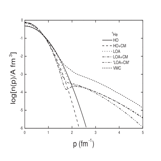
Figure 3: The momentum distribution per particle (or the generalized momentum distribution per pair for $Q=0$ (Eq.(5)) as a function of $p$ in the case of ⁴He in the simple harmonic oscillator model (HO, Eq.(21)) and with CM effects (HO+CM, Eq. (19)) as well including SRC using LOA and correlation function $g_{2}$ (LOA, Eq.(25)) and considering CM effects (LOA+CM, Eq.(26)) and approximation ’LOA+CM’ (see sec. 4.1.2). In addition, the results of the variational Monte Carlo calculation VMC [49] are plotted. A logarithmic scale is used.

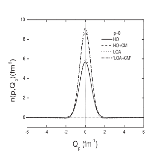
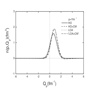
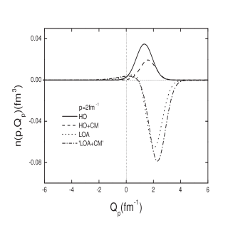
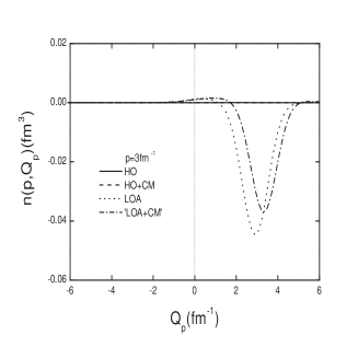
Figure 4: Generalized momentum distribution of ⁴He for $\vec{Q}$ parallel to $\vec{p}$, $n(p,Q_{p})$ as a function of $Q_{p}$ for $p=0,1,2,3$ fm^-1 in the simple harmonic oscillator (HO, eq.(20)) and with CM effects (HO+CM, eq. (17)) as well including SRC using LOA and correlation function $g_{2}$ (LOA, eq.(23)) and considering CM effects using approximation ’LOA+CM’ (see 4.1.2).

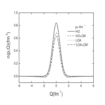
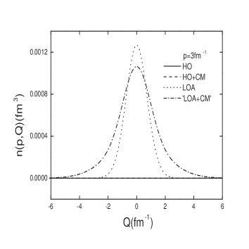
Figure 5: As in figure 4 but for $\vec{Q}$ perpendicular to $\vec{p}$ and for $p=1$ and $p=3$ fm^-1.

Some numerical results for $n(\vec{p},\vec{Q})$ of ⁴He are presented in Figs. 2-6. In Fig. 2, the GMD is plotted for $\vec{Q}$ parallel to $\vec{p}$, $\vec{Q}=Q_{p}\hat{p}$ as a function of $Q_{p}$ for $p=0,1,2$ and $3$ fm^-1. The correlated GMD calculated with the use of LOA and of the correlation functions 1G and $g_{2}$, as given by Eq. (23), is plotted by continuous and dashed lines respectively. The GMD in the harmonic- oscillator model, Eq. (20), is plotted by dotted lines. It seems that SRC within LOA contribute a negative part to $n(\vec{p},\vec{Q})$ for positive $Q_{p}$ mainly at high values of $p$. As expected, deviations from the HO picture are larger for high values of $p$ and (or) $Q_{p}$. We should recall that in infinite nuclear matter it was found that SRC are mainly significant for $|\vec{p}-\vec{Q}|>k_{F}$ and/or $p>k_{F}$ [2]. Results obtained with correlation functions 1G and $g_{2}$ are similar, but one should bear in mind that they imply about the same strength of SRC (as judged by the corresponding values of the wound parameter).

Initially the effect of the CM motion in ⁴He have been considered on the generalized momentum distribution per pair for $Q=0$ (which equals the momentum distribution per particle (Eq. (5)). In Fig. 3 the momentum distribution $n(p)$ per particle has been plotted in the single HO model (Eq. (21)) and in the HO including CM effects (HO+CM, Eq. (19)) as well as in LOA including SRC via correlation function $g_{2}$ (LOA, Eq. (25)). CM effects have been evaluated exactly (LOA+CM, Eq. (26)) and using approximation ’LOA+CM’. We realize that in ⁴He in the LOA+CM evaluation of $n(p)$ a shrinking is observed relative to its values in LOA which affects the low-medium range of $p$, while the high momentum tail is not affected. A similar shrinking occurs in the HO evaluation. In addition one notices that our approximation ’LOA+CM’ is quite satisfactory for estimating the CM effects on $n(p)$ and can be used also in the case of $n(\vec{p},\vec{Q})$. In Figs 4 and 5 the GMD is plotted for $\vec{Q}$ parallel $\vec{p}$ and for $\vec{Q}$ perpendicular to $\vec{p}$ for this case, ’LOA+CM’ approximation, as well as for LOA approximation (LOA, Eq. (23)) with correlation function $g_{2}$. For comparison, plots are shown for the simple harmonic oscillator (HO, Eq. (20)) and with CM effects (HO+CM, Eq.(17)). We realize that CM effects modify the range of values of $n(\vec{p},\vec{Q})$ and produce a similar change in LOA and HO evaluations.

In Fig. 6, a comparison is made for the GMD per particle for $\vec{Q}$ parallel to $\vec{p}$ in the case of ⁴He (continuous line) and infinite nuclear matter (diamond chain) calculated within the LOA and FHNC/0 approximation [2] respectively. The Fermi wave number $k_{F}$ of infinite nuclear matter has been taken equal to $1.3925$ fm^-1 (density $\rho^{\rm NM}=0.182$ fm^-3) and in both systems the correlation function $g_{2}$ has been used. Results are shown for $p$ equal to $0$ and $2k_{F}^{\rm NM}$. We observe qualitative and in some cases even quantitative agreement in the range where SRC are expected to dominate ($p>k_{F}$ and/or $|\vec{p}-\vec{Q}|>k_{F}$). This implies that the convergence of LOA is satisfactory. The disappearance of discontinuities in the behavior of GMD of ⁴He at $Q_{p}=|p-k_{F}|$ or $Q_{p}=|p+k_{F}|$ characterizes the transition from infinite to finite Fermi systems.

Regarding the effect of other than central correlations an estimate can be drawn for the GMD per pair for $Q=0$ (which equals $n(p)/A$, Eq. (5)). In Fig. 3 the results of calculations of $n(p)/A$ with variational Monte Carlo method [49] (dashed line) are plotted along with our results. It seems that the deviations between our results (in LOA approximation) and those of ref. [49] originate mostly from such correlations.

4.2 Approximation for heavier nuclei using LOA for ⁴He. Application to ¹⁶O

4.2.1 Approximation for heavier nuclei

In principle, one could evaluate the effect of SRC on the GMD of all $\ell$-closed shell $Z=N$ nuclei within the LOA approximation for the 2DM (Eq. (22)) using the results for the one and two-body density matrices in the harmonic oscillator model [3] and Fourier transforming according to Eq. (4). The resulting expressions even in the case of the nucleus ¹⁶O are rather long and complicated. We propose an approximation for calculating the GMD for not too heavy nuclei which makes use of the GMD of ⁴He calculated in LOA. It has been derived from a corresponding approximation that seems to be valid for the momentum distribution $n(\vec{p})$. Microscopic calculations of $n(\vec{p})$ indicate that for large values of $p$ ($p>k_{F}$) the momentum distribution per nucleon is mainly dominated by the SRC and is almost independent of $A$, whereas for small values of $p$ it is satisfactorily described within the independent particle model [48, 50, 51]. Recently, it has also been shown experimentally that the momentum distribution at high momenta has the same shape for all nuclei differing only by a scale factor [5]. Therefore, the following approximation for $n(\vec{p})$ seems reasonable for a nucleus of mass number $A$, if we use the momentum distribution per particle of the nucleus ⁴He ($A=4$)

$$n^{\rm corr-4}(\vec{p};A)=n^{0}(\vec{p};A)+\frac{A}{4}\Delta n(\vec{p};4)\ ,$$ (27)

where $n^{0}(\vec{p};A)$ and $n^{\rm corr-4}(\vec{p};A)$ are the momentum distribution in the in-dependent-particle model and including SRC respectively and $\Delta n(\vec{p};4)=n^{\rm corr}(\vec{p};4)-n^{0}(\vec{p};4))$. Using the sequential relation, Eq. (5), and the correlated GMD of the nucleus ⁴He, we can derive the corresponding approximation for GMD of the nucleus with mass number $A$

$$n^{\rm corr-4}(\vec{p},\vec{Q};A)=n^{0}(\vec{p},\vec{Q};A)+\frac{A(A-1)}{12}\Delta n(\vec{p},\vec{Q};4)\ ,$$ (28)

where $n^{0}(\vec{p},\vec{Q};A)$ and $n^{\rm corr-4}(\vec{p},\vec{Q};A)$ are the GMD in the independent-particle model and including SRC respectively and $\Delta n(\vec{p},\vec{Q};4)=n^{\rm corr}(\vec{p},\vec{Q};4)-n^{0}(\vec{p},\vec{Q};4)$. We will use LOA to evaluate $n^{\rm corr}(\vec{p},\vec{Q};4)$ (Eq. (28)) and we will call the corresponding expression of $n^{\rm corr}(\vec{p},\vec{Q};A)$ as LOA-4. The approximation (28) is valid for not large values of $A$, as it does not produce a correct asymptotic behaviour for $A\rightarrow\infty$.

4.2.2 Application to ¹⁶O

In this paper, we have applied approximation (28) to calculate the effect of SRC on the GMD of the nucleus ¹⁶O. We have considered the special case that $\vec{p}$ and $\vec{Q}$ are parallel. Results for the GMD of this nucleus within the harmonic-oscillator model, $n^{0}(\vec{p},\vec{Q};16)$, have been presented and discussed in Ref. [3]. As for $\Delta n(\vec{p},\vec{Q};4)$ we have used our results for the nucleus ⁴He within the LOA for the correlation function 1G, presented in section 4.1.2. The harmonic oscillator parameter $b$ for both nuclei ⁴He and ¹⁶O has been determined in such a way as to reproduce the experimental value of the charge r.m.s. radius ($\langle r_{\rm ch,exp}^{2}\rangle^{1/2}=1.67$ fm and $2.737$ fm respectively [46]). We found the values $1.2195$ fm and $1.7825$ fm respectively within the harmonic-oscillator model.

Some of our results are plotted in Figs. 7 and 8. Fig. 7 illustrates the variation of $n(p,Q_{p})$ as a function of $Q_{p}$ for $p=0,1.1,2$ and $3$ fm^-1. Among the values of $p$ considered, we have included the value $1.1$ fm^-1, which corresponds to the Fermi wave number $k_{F}$ in ¹⁶O [3, 49]. The results obtained with the approximation (28) and within the HO model are displayed. We realize, as expected, the effect of SRC mainly for $p>k_{F}$. Since for the description of SRC in the GMD of ¹⁶O use is made of the above evaluation of GMD of ⁴He, the conclusions drawn for their effect on the behavior of GMD of ¹⁶O are similar. Fig. 8 provides an estimate of the quality of the approximation (28), of the magnitude of the omitted higher-order terms and of the contribution of other than central correlations. The GMD per pair for $Q=0$ calculated within (28), as described above (which equals the momentum distribution per particle $n(p)/A$ according to Eq. (5)) is compared with the $n(p)/A$ calculated within variational Monte Carlo method [49] and the harmonic-oscillator model. Judging from the quite good agreement between LOA and FHNC results for the momentum distribution found in ref. [42] with the use of the same correlation function and the results presented in ref. [43] it seems that the major part of the deviation between our results and those of ref. [49] stems from other than central correlations. As mentioned in Sec. 3 the CM corrections on the GMD of ¹⁶O estimated by using suitable scaling for $\vec{p}$, $\vec{w}$ and $\vec{Q}$, or a more exact method, are expected to be small.

5 Summary and Conclusions

In summary, the study of the generalized momentum distribution $n(\vec{p},\vec{Q})$ of finite, $Z=N$, $\ell$-closed shell nuclei in their ground state that has been started in Ref. [3] within the context of the independent-particle shell model using harmonic-oscillator wave functions, was continued by including Jastrow-type correlations for investigating the effect of short-range correlations, which is expected to be important in certain regions of momenta $p$ and $Q$. First, the low-order approximation of Ref. [36] has been used and the $n(\vec{p},\vec{Q})$ of ⁴He has been evaluated using single-Gaussian correlation functions (parametrizations 1G and $g_{2}$). Significant deviations from the independent-particle picture were found for rather large values of $p$ and (or) $Q$ ($p>k_{F}$, $|\vec{p}-\vec{Q}|>k_{F}$). The convergence of LOA was explored by comparing with the results of the FHNC/0 calculation of $n(\vec{p},\vec{Q})$ of infinite nuclear matter [2] in which the same correlation function $g_{2}$ was used and it was found satisfactory in most cases. In addition, the effects of CM motion has been estimated and found not negligible and the role of correlations other than central has been brought up. Next, an approximation scheme for the evaluation of $n(\vec{p},\vec{Q})$ of heavier nuclei was proposed (Eq. (28)) that includes the effect of short-range correlations by means of the above evaluated GMD of ⁴He. Numerical results have been derived for ¹⁶O and the quality of the approximation was discussed.

Further investigation of $n(\vec{p},\vec{Q})$ of finite nuclei should consider the exact evaluation of the corrections due to the Center-of-Mass motion which are quite significant in the case of light nuclei as we have realized in the approximate treatment of ⁴He. One should start along the lines of references [44, 45] for the case of $N=Z$, l-closed nuclei. Starting from these nuclei, one must also consider to include in the calculations of $n(\vec{p},\vec{Q})$ state-dependent correlations. Another interesting direction for future work is the determination of other Fourier transforms of the two-body density matrix, for example $n(\vec{p},\vec{k},\vec{Q})$ [52, 53]. The above evaluation of $n(\vec{p},\vec{Q})$ is a first step towards more realistic calculations which include also other than Jastrow correlations. The quantity $n(\vec{p},\vec{Q})$ is mainly useful for the study of final-state interactions of struck nucleons as they propagate inside the nuclear medium in various scattering processes and for the understanding of elementary excitations of nuclei.

Figure 1: The single-Gaussian correlation functions with $c=0.76$, $\beta=0.83$ fm (1G)(continuous line) and with $c=1$, $\beta=0.6765$ fm ($g_{2}$)(dashed line) (see 4.1.2).

Figure 2: Generalized momentum distribution of ⁴He for $\vec{Q}$ parallel to $\vec{p}$, $n(p,Q_{p})$ as a function of $Q_{p}$ for $p=0,1,2,3$ fm^-1 including SRC with LOA, Eq.(23) using correlation functions 1G (continuous line) and $g_{2}$ (dashed line) and in the harmonic-oscillator model, Eq. (20) (dotted line). (see 4.1.2)

Figure 6: Generalized momentum distribution per particle for $\vec{Q}$ parallel to $\vec{p}$, $n(p,Q_{p})/A$ as a function of $Q_{p}$ for ⁴He calculated by including SRC using LOA (continuous line, Eq.(23)) and for infinite nuclear matter with Fermi wave number $k_{F}^{NM}=1.3915$ fm^-1 calculated in Fermi-hypernetted chain approximation [2] (diamond chain). In both systems the correlation function $g_{2}$ is used and results are presented for $p=0$ and $2$ $k_{F}^{NM}$.

Figure 7: Generalized momentum distribution of ¹⁶O for $\vec{Q}$ parallel to $\vec{p}$, $n(p,Q_{p})$ as a function of $Q_{p}$ for $p=0,1.1,2$ and $3$ fm^-1 including SRC using the approximation of Eq.(28) and LOA (LOA-4) and correlation function 1G (continuous line) and in the harmonic-oscillator model (dotted line).

Figure 8: Generalized momentum distribution per pair for $Q=0$ (or momentum distribution per particle (Eq. (5)) as a function of $p$, in the case of ¹⁶O, including SRC using the approximation of Eq.(28) and LOA (LOA-4) and correlation function 1G (continuous line) along with the results for the momentum distribution per particle of a variational Monte Carlo calculation [49] (dashed line, VMC) and of the harmonic-oscillator model (dotted line). A logarithmic scale is used.

References

- [1] Ristig M L and Clark J W 1990 Phys. Rev. B 41 8811
- [2] Mavrommatis E, Petraki M and Clark J W 1995 Phys. Rev. C 51 1849
- [3] Papakonstantinou P, Mavrommatis E and Kosmas T S 2000 Nucl. Phys. A 673 171
- [4] Arrington J et al. 1999 Phys. Rev. Lett. 82 2056
- [5] Egiyan K S et al. 2003 Phys. Rev. C 68 014313
- [6] Carroll A S et al. 1988 Phys. Rev. Lett. 61 1698
- [7] Abbott D et al. 1998 Phys. Rev. Lett. 80 5072
- [8] Kozlov A (A1 Collaboration) 2000 Ph.D Thesis University of Melbourne
- [9] Reitz B 2004 Eur. Phys. J. A 19 S01 165
- [10] Gao J et al. 2000 Phys. Rev. Lett. 84 3265
- [11] Fissum K et al. 2004 Phys. Rev. C 70 034606
- [12] Garrow K R et al. 2002 Phys. Rev. C 64 064602
- [13] Dutta D et al. 2003 Phys. Rev. C 68 064603
- [14] Stavinsky A V et al. (CLAS collaboration) 2004 Phys. Rev. Lett. 93 192301
- [15] Rohe D et al. (E97-006 collaboration) 2004 Phys. Rev. Lett. 93 182501
- [16] Niyazov R A et al. 2004 Phys. Rev. Lett. 92 052303
- [17] Annand J R et al. 1993 Phys. Rev. Lett. 71 2703
- [18] Mardor I et al. 1998 Phys. Rev. Lett. 81 5085
- [19] Leksanov A et al. 2001 Phys. Rev. Lett. 87 212301
- [20] Aclander J et al. 2004 Phys. Rev. C 70 015208
- [21] Braghieri A, Giusti C and Grabmayr P (Eds) 2003 Proceedings of the 6th Workshop in Electromagnetically Induced Two-Hadron Emission, Pavia, Italy, Sept. 24-27, and refs. therein
- [22] Walcher T 2003 Prog. Part. Nucl. Phys. 50 503
- [23] Jlab experiments: E00-102, E01-015, E02-019
- [24] Petraki M, Mavrommatis E, Benhar O, Clark J W, Fabrocini A and Fantoni S 2003 Phys. Rev. C 67 014605
- [25] Mazzanti F 1997 PhD Thesis University of Barcelona
- [26] Chiofalo M L, Conti S and Tosi M P 1996 J. Phys.: Condens. Mattter 8 1921
- [27] Stringari S 1992 Phys. Rev. B 46 2974
- [28] Clark J W, Mavrommatis E and Petraki M 1993 Acta Phys. Pol.B 24 659
- [29] Petraki M, Mavrommatis E and Clark J W 2001 Phys. Rev. C 64 024301
- [30] Kosmas T S and Vergados J D 1990 Nucl. Phys. A 510 641
- [31] Kosmas T S and Vergados J D 1992 Nucl. Phys. A 536 72
- [32] Papakonstantinou P 1998 Msc Thesis University of Athens
- [33] Papakonstantinou P, Mavrommatis E and Kosmas T S 2003 Nucl. Phys. A 713 81
- [34] Gaudin M, Gillespie J and Ripka G 1971 Nucl. Phys. A 176 237
- [35] Bohigas O and Stringari S 1980 Phys. Lett. B 95 9
- [36] Dal Ri M, Stringari S and Bohigas O 1982 Nucl. Phys. A 376 81
- [37] Stoitsov M V, Antonov A N and Dimitrova S S 1993 Phys. Rev. C 48 74
- [38] Massen S E and Moustakidis Ch C 1999 Phys. Rev. C 60 024005
- [39] Moustakidis Ch C and Massen S E 2000 Phys. Rev. C 62 034318
- [40] Dimitrova S S, Kadrev N D, Antonov A N and Stoitsov M V 2000 Eur. Phys. Journ. A 7 335
- [41] Orlandini G and Sara L May 17-20 1995 In Proceedings of the Second Workshop on Electromagnetically Induced Two-Nucleon Emission Gent p1.
- [42] Arias de Saavedra F, Cò G and Renis M M 1997 Phys. Rev. C 55 673
- [43] Alvioli M, Ciofi degli Atti C and Morita H 2005 Phys. Rev. C 72 054310
- [44] Shebeko A, Papakonstantinou P and Mavrommatis E 2006 Eur. Phys. J. A 27 143
- [45] Shebeko A, et al. 2007 to appear in EPJA.
- [46] De Vries H, De Jager C W and De Vries C 1987 At. Data Nucl. Data Tables 36 495
- [47] Mavrommatis E, Petraki M, Papakonstantinou P, Kosmas T S and Moustakidis Ch C 2001 Proceedings of the Conference “150 years of Quantum Many-Body Physics” UMIST p.177
- [48] Flynn M F, Clark J W, Panoff R M, Bohigas O and Stringari S 1984 Nucl. Phys. A 427 253
- [49] Pieper S C, Wiringa R B and Pandharipande V R 1992 Phys. Rev. C 46 1741
- [50] Zabolitzky J G and Ey W 1978 Phys. Lett. B 76 527; Arias de Saavedra F, Cò G, Fabrocini A and Fantoni S 1996 Nucl. Phys. A 605 359
- [51] Antonov A N, et al. 2005 Phys. Rev. C 71 014317
- [52] Ristig M L and Clark J W 1989 Phys. Rev. B 40 4355
- [53] Moustakidis Ch C and Mavrommatis E in preparation