Near threshold $NN\to d\pi$ reaction in chiral perturbation theory

Abstract

The near-threshold $np\to d\pi^{0}$ cross section is calculated in chiral perturbation theory to next-to-leading order in the expansion parameter $\sqrt{Mm_{\pi}}/{\Lambda_{\chi}}$. At this order irreducible pion loops contribute to the relevant pion-production operator. While their contribution to this operator is finite, considering initial- and final-state distortions produces a linear divergence in its matrix elements. We renormalize this divergence by introducing a counterterm, whose value we choose in order to reproduce the threshold $np\rightarrow d\pi^{0}$ cross section measured at TRIUMF. The energy-dependence of this cross section is then predicted in chiral perturbation theory, being determined by the production of $p$-wave pions, and also by energy dependence in the amplitude for the production of $s$-wave pions. With an appropriate choice of the counterterm, the chiral prediction for this energy dependence converges well.

I Introduction

Ever since the days of current algebra, soft-pion theorems, which relate processes involving different numbers of pions, have been used to understand threshold pion-production reactions KR ; SSY . These relations originate from the chiral symmetry of the underlying Lagrangian of quantum chromodynamics (QCD) and have now been systematized into an effective field theory called chiral perturbation theory ($\chi$PT) We79 ; ulfreview . In $\chi$PT, there is not only an understanding of these relations between amplitudes, but also an organizing principle (power counting), which suggests a hierarchy of contributions to the amplitudes and thus makes it possible to assign a theoretical error to a calculation. $\chi$PT can be regarded as an extension of and improvement on current algebra and it has found many applications. Significant progress has been made in the pion-pion and pion-nucleon sectors (for a review of the latter see ulfreview ) and for nucleon-nucleon scattering Weinberg ; bira ; evgeny . Here we will apply it to threshold pion production in few-nucleon systems.

The application of chiral perturbation theory to threshold pion-production reactions has met with mixed success. In the charged-pion production reactions the leading pion rescattering mechanism involves the Weinberg-Tomozawa (WT) $\pi N$ amplitude. Considering this, plus certain higher-order effects, produces moderate agreement between theory and data cross sections dRMvK . Approaches to these reactions based on meson-exchange models are also quite successful CHpolpi ; Teresa .

Meanwhile, both meson-exchange models and $\chi$PT initially struggled to describe the $pp\to pp\pi^{0}$ cross section measured close to threshold. Data from the Indiana University Cyclotron Facility Meyer and the The Svedberg Laboratory in Uppsala, Sweden TSL were five times larger than phenomenological calculations Miller . Two early proposals to remedy this deficiency were short-range interactions LeeRiska ; Chucketal and $\pi N$ amplitudes with a particular off-shell dependence Oset . In $\chi$PT these effects are both higher order, and they are related to each other through field redefinitions Cohen . This sensitivity to higher-order effects is partly a consequence of the particular isospin structure of the $pp\to pp\pi^{0}$ reaction, which forbids the pion rescattering via the WT term that is the leading effect in the charged-pion channels. (In $\chi$PT there is also a partial cancellation between higher-order one-body and rescattering terms, which is not present in meson-exchange model treatments Cohen ; Pa96 ; USC1 ; USC2 .) But even at a formal level, it quickly became apparent that the conventional $\chi$PT expansion of amplitudes in $\frac{m_{\pi}}{M}$ (with $M$ and $m_{\pi}$ the nucleon and pion masses) does not apply to pion production in few-nucleon systems, since the initial nucleons have a large relative momentum $P=\sqrt{Mm_{\pi}+\frac{m_{\pi}^{2}}{4}}\sim 360$ MeV/c. Because of this an expansion in $P/M=\sqrt{m_{\pi}/M}\sim 0.4$ was adopted Cohen . But the convergence of this expansion is slow, and it is necessary to include several poorly constrained higher-order mechanisms in order to achieve a good description of the data, e.g., the short-range interactions and/or off-shell amplitudes mentioned above vK96 . These effects are included in meson-exchange-model calculations of $pp\to pp\pi^{0}$, but even so such calculations struggle to describe spin observables CHpolpi ; IUCFpolpp . The present situation, with a detailed review of this interesting field, is given in Ref. CHreview . As that review points out, in spite of its difficulties, the $\chi$PT expansion in powers of $\sqrt{m_{\pi}/M}$ does predict the correct hierarchy of mechanisms for the production of pions in a relative $s$-wave. It also successfully explains $p$-wave pion production CHp .

The $np\to d\pi^{0}$ reaction is of particular and current interest. The total cross section was measured some time ago at TRIUMF Hutcheon , and fitted to the expression

$$\sigma(np\to d\pi^{0})=\frac{1}{2}(\alpha\eta+\beta\eta^{3}),$$ (1)

where $\eta\equiv q/m_{\pi}$ is the reduced c.m. pion momentum and Ref. Hutcheon gives the values $\alpha=184\pm 5~{}\mu$b and $\beta=781\pm 79~{}\mu$b for what they call the reduced (pion) $s$- and $p$-wave cross sections (but see also below). The factor $1/2$ results from a comparison with the (Coulomb corrected) isospin partner $pp\to d\pi^{+}$. The $\pi^{+}d\to pp$ data (applying detailed balance) are in agreement with $np\to d\pi^{0}$ Ritchie . However, more recent data on the $pp\to d\pi^{+}$ reaction gives $\alpha=208\pm 5$ $\mu$b, $\beta=1220\pm 100$ $\mu$b Heimberg and $\alpha=205\pm 9$ $\mu$b, $\beta=791\pm 79$ $\mu$b Drochner , indicating a possible isospin violation. A model calculation Chuck managed to reproduce the data of Ref. Hutcheon , but it was subsequently pointed out that Ref. Chuck overestimated contributions from short-range pion-production mechanisms Jouni . More recently the charge-symmetry-breaking (CSB) forward-backward asymmetry was measured to be $A_{\rm fb}=[17.2\pm 8({\rm stat})\pm 5.5({\rm sys})]\times 10^{-4}$ Allena . The asymmetry is an interference between charge independent (CI) and CSB $s$- and $p$-waves. Ignoring relative phases it can be expressed as

$$A_{\rm fb}(np\to d\pi^{0})\sim\frac{\sqrt{\alpha\widetilde{\beta}}\eta^{2}+\sqrt{\widetilde{\alpha}\beta}\eta^{2}}{\alpha\eta+\beta\eta^{3}}\approx\sqrt{\frac{\widetilde{\beta}}{\alpha}}\eta+\frac{\sqrt{\widetilde{\alpha}\beta}}{\alpha}\eta,$$ (2)

where $\widetilde{\alpha}$ and $\widetilde{\beta}$ are the CSB equivalents of $\alpha$ and $\beta$. It is believed that this asymmetry, together with the recent $5\sigma$ result of the $dd\to\alpha\pi^{0}$ experiment IUCFCSB , will help constrain some of the lesser known, but important, CSB parameters in the chiral Lagrangian vKNM ; CSB1 . For this reason there is a need for consistent chiral calculations for both reactions. A first report on the demanding $dd\to\alpha\pi^{0}$ calculation has been published CSB1 , and a calculation incorporating some of the physics mandated by chiral symmetry that affects $A_{\rm fb}(np\to d\pi^{0})$ exists vKNM , but a reliable extraction of CSB parameters necessitates a consistent chiral calculation of the reaction $np\to d\pi^{0}$.

In this paper we will use the power counting appropriate for pion production to establish the leading- and next-to-leading-order (LO and NLO) diagrams that contribute to the CI $s$-wave $np\to d\pi^{0}$ amplitude close to threshold. This is a preparatory, but important, step toward the calculation of the CSB asymmetry, since Eq. (2) makes it clear that without an understanding of the CI cross section the asymmetry is not under control.

The organization of the paper is as follows. We introduce the theoretical framework in Sec. II. The LO operator and results are presented in Sec. III, while the NLO operator is introduced in Sec. IV. The results at this order are discussed in Sec. V, and the energy dependence of the $s$-wave cross section in Sec. VI. We conclude in Sec. VII.

II Theory

II.1 General considerations

The $np\to d\pi^{0}$ reaction can easily be decomposed into partial waves. The lowest CI partial waves are ${}^{3}P_{1}s$, ${}^{1}S_{0}p$, and ${}^{1}D_{2}p$ in the spectroscopic notation ${}^{2S+1}L_{J}l_{\pi}$, where $S$, $L$, and $J$ are the total spin, orbital, and total angular momentum of the incoming nucleon pair and $l_{\pi}$ is the orbital angular momentum of the emerging pion. The lowest CSB partial waves are ${}^{1}P_{1}s$, ${}^{3}S_{1}p$, ${}^{3}D_{1}p$, and ${}^{3}D_{2}p$.

As we will restrict ourselves to near-threshold CI $s$-wave pion production, only the ${}^{3}P_{1}s$ transition will be evaluated in this paper. This wave contributes to $\alpha$, while ${}^{1}S_{0}p$ and ${}^{1}D_{2}p$ both contribute to $\beta$. Note, however, that $\alpha$ and $\beta$ do not give an unambiguous separation of $s$- and $p$-waves. An $s$-wave amplitude that is dependent on the pion energy, e.g., the WT term, will produce a term quadratic in $\eta$. This term’s interference with the $\eta$-independent piece of the ${}^{3}P_{1}s$-wave amplitude mimics the $\eta^{3}$ dependence of $p$-wave contributions to $\sigma$. A separation of the $\eta^{2}$ piece of the ${}^{3}P_{1}s$-wave amplitude and the $p$-wave contributions can be made using the energy dependence of the analyzing power $A_{y}$. Defining the calculated $s$- and $p$-wave contributions $\bar{\alpha}(\eta)$ and $\bar{\beta}(\eta)$, their energy dependence can be written as

$$\bar{\alpha}(\eta) = \bar{\alpha}_{0}+\bar{\alpha}^{\prime}\eta^{2},$$

$$\bar{\beta}(\eta) = \bar{\beta}_{0}+\bar{\beta}^{\prime}\eta^{2},$$ (3)

and the analyzing power as (again ignoring relative phases)

$$A_{y}=\frac{\sqrt{\bar{\alpha}_{0}+\bar{\alpha}^{\prime}\eta^{2}}\sqrt{\bar{\beta}_{0}+\bar{\beta}^{\prime}\eta^{2}}\eta^{2}}{(\bar{\alpha}_{0}+(\bar{\alpha}^{\prime}+\bar{\beta}_{0})\eta^{2})\eta}\approx\sqrt{\frac{\bar{\beta}_{0}}{\bar{\alpha}_{0}}}\eta\left[1+\left(\frac{\bar{\beta}^{\prime}}{2\bar{\beta}_{0}}-\frac{\bar{\alpha}^{\prime}}{2\bar{\alpha}_{0}}-\frac{\bar{\beta}_{0}}{\bar{\alpha}_{0}}\right)\eta^{2}\right].$$ (4)

This expansion is valid as long as $\frac{\bar{\alpha}^{\prime}}{\bar{\alpha}_{0}}\eta^{2}\ll 1$, $\frac{\bar{\beta}^{\prime}}{\bar{\beta}_{0}}\eta^{2}\ll 1$, and $\frac{\bar{\alpha}^{\prime}+\bar{\beta}_{0}}{\bar{\alpha}_{0}}\eta^{2}\ll 1$. (In fact, existing data for $pp\to d\pi^{+}$ are consistent with $A_{y}\propto\eta$ for $\eta<0.5$ ppdpi .)

With our normalization, the total $np\to d\pi^{0}$ cross section is

$$\sigma=\frac{\eta}{2}\frac{m_{n}m_{p}}{4\pi^{2}s}\frac{m_{\pi}}{p}\frac{1}{4}\sum_{\rm spins}|\mathcal{M}|^{2},$$ (5)

where ${\bf p}$ is the relative c.m. momentum of the incoming nucleons, $\sqrt{s}$ is the total energy in the c.m. system, and the sum is over the nucleon and deuteron spins. A general form for the $np\to d\pi^{0}$ matrix element, $\mathcal{M}$, in $p$-space, is then

$$\mathcal{M}=\sqrt{2E_{d}}\int\frac{d^{3}p^{\prime\prime}d^{3}p^{\prime}}{(2\pi)^{6}}\psi_{d}^{\dagger}({\bf p}^{\prime\prime})\mathcal{A}(\tilde{\bf p})\psi_{np}({\bf p}^{\prime},{\bf p}),$$ (6)

where $E_{d}$ is the deuteron energy, $\psi_{d}({\bf p}^{\prime\prime})$ and $\psi_{np}({\bf p}^{\prime},{\bf p})$ are the deuteron and $np$ wave functions, $\tilde{\bf p}={\bf p}^{\prime\prime}-{\bf p}^{\prime}$, and $\mathcal{A}(\tilde{\bf p})$ is the pion-production amplitude. A recurring problem in any calculation of threshold pion-production amplitudes is the mismatch between initial- and final-state nucleon momenta. Since the initial loop momentum $p^{\prime}\sim p\sim P\approx 360$ MeV, while the final loop momentum $p^{\prime\prime}\sim 45$ MeV, the two integrals in the matrix element need to be performed in quite different momentum domains. Critical questions are: Where is the large initial-state momentum absorbed in order to effect the transition between the two regimes? Does it have to pass through the deuteron wave function or are there pieces of the operator that can help absorb it?

II.2 Chiral perturbation theory

We will use the “hybrid” approach to derive the $\chi$PT prediction for $np\rightarrow d\pi^{0}$ at threshold. In this approach chiral power counting is applied to the transition operator $\mathcal{A}$. The wave functions in Eq. (6) account for the effects of initial- and final-state nucleons propagating nearly on their mass shell. Such states have small energy denominators that do not obey the usual $\chi$PT power counting Weinberg . Thus they have to be calculated non-perturbatively, ideally in a manner consistent with chiral symmetry. The hybrid approach has been applied successfully to a wide range of pionic and electroweak reactions in the two-nucleon system (see Refs. Be00 ; birareview ; Ph05 for reviews).

We use the chiral Lagrangian as developed in Ref. Cohen , Eqs. (3) and (6). These contain pieces from the first and second chiral orders, which is all we need for the present purposes. The chiral Lagrangian is used to construct the transition operator ${\cal A}$ in Eq. (6), which is just the sum of all of the two-nucleon-irreducible diagrams that contribute to $NN\rightarrow NN\pi$. These diagrams are arranged using a power counting which involves a number of different energy/momentum scales. Ordered by size these scales are:

• The pion momentum $|{\bf q}|$ which is $\ll m_{\pi}$ close to threshold. At NLO (which is all we consider here), this scale does not enter the $s$-wave production amplitude.

• The deuteron binding momentum $\gamma\equiv\sqrt{BM}=45$ MeV, where $B$ is the deuteron binding energy. We expect that the integral over ${\bf p}^{\prime\prime}$ in Eq. (6) will be dominated by $|{\bf p}^{\prime\prime}|\sim\gamma$. However, here we will conservatively adopt $|{\bf p}^{\prime\prime}|\sim m_{\pi}$.

• The pion mass $m_{\pi}$ for which we take $138.039$ MeV.

• The Delta-isobar–nucleon mass difference $\Delta=M_{\Delta}-M=290\ {\rm MeV}\approx 2m_{\pi}$.

• The nucleon momentum needed to produce a pion at threshold $P\equiv\sqrt{m_{\pi}(M+m_{\pi}/4)}=360$ MeV.

• The chiral symmetry breaking scale $\Lambda_{\chi}\sim 1$ GeV.

We will see below that the scale $\Delta$ will never appear explicitly in the tree-level diagrams, since it will be combined with the pion mass in propagators. Meanwhile, in loop diagrams involving the Delta-isobar, we follow Ref. HK and assign $\Delta\sim P$.

Thus we have a three-scale problem, with the hierarchy $m_{\pi}\ll P\ll\Lambda_{\chi}$. We choose to expand our amplitudes in the dimensionless parameter

$$x=\frac{m_{\pi}}{P}=\sqrt{\frac{m_{\pi}}{M}}\approx\frac{P}{\Lambda_{\chi}}\approx 0.4.$$ (7)

When counting powers of $x$ in two-nucleon-irreducible loop diagrams it is important to distinguish between graphs of the type in Fig. 1 and those of the type shown in Fig. 3. In the first case the large nucleon momentum $P$ may pass through the nucleons and exchanged pions only (Fig. 1), whereas in the second it must go through pions in a loop [e.g., Fig. 3(a)–(h)].

Figure 1: Examples of diagrams where the large momentum need not appear in a pion loop.

In consequence the loops in Fig. 1 are independent of the initial nucleon momentum $P$, since the loop resides only on a nucleon which is moving with momentum $P$. By translation invariance, the loop integral then scales with $m_{\pi}$ only. In Fig. 3 the loop integrals pick up the large momentum scale and the integral will be dominated by pion modes of momentum $P$.

II.3 Wave functions consistent with chiral symmetry

In evaluating the matrix element (6) we would like to employ wave functions which are consistent with the chiral power counting that we use for the operators. One way to do this for the deuteron was developed in Ref. PC . This method was extended to $NN$ scattering in EFTann . In these wave functions the long-range part of the $NN$ potential is derived using $\chi$PT Weinberg ; bira ; evgeny . At the same time our ignorance about the short-distance physics of the nucleon-nucleon interaction is parametrized by matching, at some chosen radius $R$, the wave function obtained for $r>R$ to a square well solution for $r<R$. Here we will use this approach to construct the initial-state $np$ wave function, starting from the ${}^{3}P_{1}$ $np$ phase shift of the Nijmegen phase shift analysis NijmPSA . Since we are dealing with c.m. energies of order $m_{\pi}$, we determine the asymptotic scattering wave functions from the Nijmegen phase shifts at a lab. energy of 279.5 MeV and then expand around this point. This is different from the procedure chosen in EFTann , where, due to the low $NN$ energy, the $nn$ scattering length and effective range could be used as input. Note that, at the present state of the calculation, we include only one-pion exchange (OPE) with $f_{\pi NN}^{2}=0.075$ NijmpiNN as the long-range part of the chiral $NN$ potential. In the future we will also implement chiral two-pion exchanges (TPE) bira ; evgeny ; RTFdS . (Unfortunately, it is impossible to use high-order chiral potentials directly, since in general they are accurate only for energies below 250 MeV evgeny ; EM .) As a cross check, below we also use some of the available low-$\chi^{2}$ potential model wave functions NijmPot ; av18 to calculate the matrix element (6).

The chiral wave functions we have constructed for use in our calculation have a co-ordinate space regulator present in them: the square well of radius $R$. Other regulators (e.g., Gaussians or sharp cutoffs in momentum space) have been used in obtaining $NN$ wave functions from a potential derived via a $\chi$PT expansion bira ; evgeny ; Pa99 ; BBSvK01 ; No05 . In all of these studies a regulator is introduced before the potential is iterated using the Schrödinger equation. This means that when, in Eq. (6), matrix elements of pion-production operators are computed using such wave functions, there is a scale-dependent regularization in the ${\bf p}^{\prime}$ and ${\bf p}^{\prime\prime}$ integrations. The scale dependence of this regularization is less obvious when $NN$ potential models are used to calculate the $\psi$’s appearing in Eq. (6). However, even there it seems clear that the hadronic form factors in such models somehow implicitly provide a regularization that is explicitly present when wave functions derived from the effective field theory are used.

III Leading-order operator and result

The LO [or $\mathcal{O}(x)$] $s$-wave operator is given by the Weinberg-Tomozawa (WT) and the (nucleon recoil) one-body term;

$$\mathcal{A}_{\rm WT}(\tilde{\bf p}) = \frac{3g_{A}\omega_{q}}{16f_{\pi}^{3}}\varepsilon^{abc}\tau_{1}^{b}\tau_{2}^{c}\left(\frac{\mbox{\boldmath${\sigma}$}_{1}\cdot(\tilde{\bf p}-\frac{{\bf q}}{2})}{{m_{\pi}^{\prime}}^{2}+(\tilde{\bf p}-\frac{{\bf q}}{2})^{2}}+\frac{\mbox{\boldmath${\sigma}$}_{2}\cdot(\tilde{\bf p}+\frac{{\bf q}}{2})}{{m_{\pi}^{\prime}}^{2}+(\tilde{\bf p}+\frac{{\bf q}}{2})^{2}}\right),$$

$$\mathcal{A}_{\rm 1B}(\tilde{\bf p}) = \frac{-ig_{A}\omega_{q}(2\pi)^{3}}{4Mf_{\pi}}\left[\tau_{1}^{a}\delta^{(3)}\left(\tilde{\bf p}+\frac{{\bf q}}{2}\right)\mbox{\boldmath${\sigma}$}_{1}\cdot\left({\bf p}^{\prime\prime}+{\bf p}^{\prime}-\frac{{\bf q}}{2}\right)\right.$$ (8)

$$\left.-\tau_{2}^{a}\delta^{(3)}\left(\tilde{\bf p}-\frac{{\bf q}}{2}\right)\mbox{\boldmath${\sigma}$}_{2}\cdot\left({\bf p}^{\prime\prime}+{\bf p}^{\prime}+\frac{{\bf q}}{2}\right)\right],$$

where ${m_{\pi}^{\prime}}^{2}=\frac{3}{4}(m_{\pi}^{2}-q^{2})$. [In order to derive Eq. (8) we have assumed equal energy sharing between the two nucleons.]

Chiral power counting for the operator ${\cal A}$ will be a useful guide to the size of physical mechanisms only if different contributions to the operator are sensitive to similar momenta in the $NN$ wave functions used in the evaluation of the matrix element (6). This is clearly not the case for the operators in Eq. (8): the one-body operator “lives” off the high-momentum components in the incoming state, while the two-body nature of the pion-rescattering mechanism allows better momentum sharing, and access to the larger low-momentum components in the $np$ and $d$ wave functions. Therefore in order to estimate the impact the operator ${\cal A}_{\rm 1B}$ has on observables we follow Ref. Cohen and use the Schrödinger equation for the deuteron state $|\psi_{d}\rangle$ to write

$$\langle\psi_{d}|{\cal A}_{\rm 1B}|\psi_{np}\rangle=\langle\psi_{d}|VG_{0}{\cal A}_{\rm 1B}|\psi_{np}\rangle.$$ (9)

(Here $V$ is the $NN$ potential used to generate the wave functions.) Once Eq. (9) is invoked momentum sharing can take place through $V$. So, in order to power count the operator ${\cal A}_{\rm 1B}$, the pion exchange and contact interaction that make up $V$ at leading order in $\chi$PT Weinberg are included in the diagrams. This also puts the nucleons in the “external” states closer to being on-shell, and facilitates attaching wave functions that are calculated assuming on-shell nucleons.

Figure 2: Leading-order diagrams for $s$-wave pion production on two nucleons.

The diagrams in Fig. 2 are then the same order in chiral power counting, which justifies the statement made at the beginning of this section that ${\cal A}_{\rm 1B}$ and ${\cal A}_{\rm WT}$ together give the leading-order amplitude. This statement is borne out if we compute the different contributions to $\bar{\alpha}_{0}$ from these leading-order processes using a variety of phenomenological and chiral wave functions NijmPot ; av18 ; Bonn ; PC . The results of that computation are shown in Table 1.

Table 1: Values for $\bar{\alpha}_{0}$ obtained from various different contributions to the leading-order $np\rightarrow d\pi^{0}$ amplitude. All results are in units of $\mu$b. Note that in each case (except the last column) the result for $\bar{\alpha}_{0}$ is the one obtained by considering just that mechanism.

potential	$\bar{\alpha}_{0}$(WT)	$\bar{\alpha}_{0}$(1B, PWIA)	$\bar{\alpha}_{0}$(1B, ISI)	$\bar{\alpha}_{0}$(1B)	$\bar{\alpha}_{0}$(LO)
Nijm I	124.0	11.94	11.83	0.0003	123.6
Nijm II	96.8	16.26	18.21	0.0682	102.0
av18	82.2	15.75	22.35	0.6961	98.1
Bonn A	111.8	6.264	9.622	0.4234	126.0
Bonn B	110.4	11.28	12.96	0.0713	116.0
LO $\chi$PT ($R=1.5$ fm)	40.6	5.809	19.90	4.723	73.0
LO $\chi$PT ($R=2$ fm)	114.7	1.124	9.391	4.325	163.6

Considering that the power counting predicts the WT and one-body term to be of the same order, the six order of magnitude difference between the two in the first row of Table 1 should cause some concern. However, we can split up the matrix element of ${\cal A}_{\rm 1B}$ into a plane-wave (PWIA) and initial-state-interaction (ISI) part, i.e., write:

$$\langle\psi_{d}|{\cal A}_{\rm 1B}|\psi_{np}\rangle=\langle\psi_{d}|{\cal A}_{\rm 1B}|{\bf p}\rangle+\langle\psi_{d}|{\cal A}_{\rm 1B}G_{0}V|\psi_{np}\rangle.$$ (10)

The fact that the PWIA and ISI contributions to $\bar{\alpha}_{0}$ are of the same size lends credence to our application of power counting to the pion-production operator. The one-body ISI and PWIA values alone are closer to the $\bar{\alpha}_{0}$ from the WT mechanism than is their sum, although each piece still differs from $\bar{\alpha}_{0}$(WT) by an order of magnitude. The extremely small matrix element on the left-hand side of Eq. (10) apparently results from a cancellation between two numbers of a little smaller than natural size on the right-hand side of that equation. The total LO value for $\bar{\alpha}_{0}$ is then quite close to the number from Fig. 2(a) alone.

The numbers in Table 1 are in accord with those given in the earlier study of da Rocha et al. dRMvK . (Cancellations between different pieces of the integral, leading to a reduction in the one-body term, were also observed in Ref. dRMvK , although there the PWIA and ISI contributions are not given separately.)

We find that there is considerable wave-function dependence in the result for $\bar{\alpha}_{0}$. The calculation with the chiral wave function with cutoff $R=1.5$ fm is expected to differ from the other results, since at $p=360$ MeV the matrix element will probe distances where the neglected TPEs become important. If we employ only the low-$\chi^{2}$ $NN$ potential models we find a moderate spread in values:

$$\bar{\alpha}_{0}=111\pm 13~{}\mu{\rm b}.$$ (11)

This variation with the choice of $NN$ model reflects the sensitivity to short-distance physics in the LO pion-production matrix element, since these potentials reproduce the 1993 $NN$ database with $\chi^{2}\approx 1$ and have the same OPE tail. The LO prediction (11) gives $\approx 60\%$ of the measured $\alpha$, which is consistent with the accuracy expected from a LO result in an expansion in $\sqrt{m_{\pi}/M}$.

The use of wave functions derived assuming zero-energy transfer between the nucleons means that there is an inconsistency between these wave functions and the operator. In diagram 2(b), for example, we assume there is energy transfer between the nucleons, as dictated by the Feynman rules and our assumption of equal-energy sharing between the initial particles. If the procedure used here and in Ref. Cohen for power counting diagrams by “pulling” the last pion exchange from the wave functions is accurate then this inconsistency should be a higher-order effect, since it involves the difference

$$\frac{1}{{m_{\pi}^{\prime}}^{2}+(\tilde{\bf p}\pm\frac{{\bf q}}{2})^{2}}-\frac{1}{{m_{\pi}}^{2}+(\tilde{\bf p}\pm\frac{{\bf q}}{2})^{2}}=\frac{m_{\pi}^{2}-{m_{\pi}^{\prime}}^{2}}{{m_{\pi}}^{2}+(\tilde{\bf p}\pm\frac{{\bf q}}{2})^{2}}\times\frac{1}{{m_{\pi}^{\prime}}^{2}+(\tilde{\bf p}\pm\frac{{\bf q}}{2})^{2}}.$$ (12)

The momentum transferred here is of order $P$, so the difference between including and not including energy transfer in the one-pion-exchange propagator is of relative order $\left(\frac{m_{\pi}}{P}\right)^{2}$, as long as $q\sim m_{\pi}$. It therefore contributes first at two orders beyond leading, which is one order higher than we consider here.

Similar arguments ensure that any $\eta$ dependence of the leading-order $s$-wave production amplitude ${\cal A}_{s}$ arising from energy flowing through these meson denominators is also a NNLO effect. Thus

$$\mathcal{A}_{s}=\omega_{q}\left[\widetilde{\mathcal{A}}_{s}+\mathcal{O}(x^{2}\eta^{2})\right],$$ (13)

where $\widetilde{\mathcal{A}}_{s}$ is the reduced leading order $\mathcal{A}_{S}$ and the $\mathcal{O}(x^{2}\eta^{2})$ correction stems from the ${\bf q}$ dependence of the vertices and propagators in Eq. (8). Thus the prediction of $\chi$PT for these diagrams (13) is that (ignoring ISI for the moment)

$$\sigma=\frac{\eta}{2}\bar{\alpha}_{0}[1+\eta^{2}+\mathcal{O}(x^{2}\eta^{2})],$$ (14)

which implies that $\bar{\alpha}^{\prime}=\bar{\alpha}_{0}$ at LO. However, a numerical calculation including the full scattering state reveals that

$$\bar{\alpha}^{\prime}=-57\pm 4~{}\mu{\rm b}$$ (15)

for the potential models, and somewhat smaller, but positive ($\bar{\alpha}^{\prime}=41\pm 30$ $\mu$b), for the chiral wave functions. The energy dependence coming from ISI apparently provides a $\gtrsim 100\%$ correction to Eq. (14). We will return to this issue of energy dependence once the NLO contributions have been calculated.

IV Next-to-leading order operator

At NLO [or $\mathcal{O}(x^{2})$], there are pion loops and a Delta-isobar–excitation term. The corresponding diagrams are shown in Fig. 3. Some of these were discussed in Ref. novel , and a complete treatment can be found in Ref. USC2 . Here we draw on the analysis of Hanhart and Kaiser HK for the pion loops shown in Fig. 3, since for these graphs they employed the power counting in $x$ we are using here.

Figure 3: Next-to-leading-order diagrams (with no Delta-isobars in loops) for $s$-wave pion production on two nucleons.

At NLO and in threshold kinematics diagrams 3(b) and 3(c) cancel for $NN\to d\pi$, while 3(e) and 3(f) $\propto m_{\pi}\ln m_{\pi}$, and thus are of higher order HK . Diagrams 3(g) and 3(h) are also of higher order in the $x$ expansion because of their vertex structure. As for diagram 3(i), since the deuteron is isoscalar this particular Delta-isobar diagram cannot contribute to $NN\to d\pi$.

There are also a number of Delta-isobar loop diagrams which nominally appear at NLO, but they cancel each other in threshold kinematics. This is associated with the absence of a chirally-invariant counterterm at this order HK . Thus for $s$-wave pion production in $np\to d\pi^{0}$, there are only two loop graphs that need to be calculated if an answer accurate to $\mathcal{O}(x^{2})$ is desired.

The sum of these two diagrams (a) and (d) can be evaluated straightforwardly. The corresponding amplitude, together with that for the analogous diagrams in which the roles of nucleons 1 and 2 are interchanged, gives the following result for the operator mediating the $NN\to d\pi$ transition:

$$\mathcal{A}_{\rm(a)+(d)}(\tilde{\bf p})=\frac{1}{2}(\mbox{\boldmath${\sigma}$}_{1}+\mbox{\boldmath${\sigma}$}_{2})\cdot\tilde{\bf p}(i\tau_{1}^{a}-i\tau_{2}^{a})B(-|\tilde{\bf p}|^{2}),$$ (16)

with $g_{A}$ the axial coupling of the nucleon, $f_{\pi}$ the pion decay constant, and $B$ given by the scalar integral

$$B(\tilde{p}^{2})\equiv\frac{g_{A}^{3}}{8f_{\pi}^{5}}\frac{1}{i}\int\frac{d^{4}q}{(2\pi)^{4}}\frac{(q+\tilde{p})\cdot q}{v\cdot q\,[(\tilde{p}+q)^{2}-m_{\pi}^{2}]\,[q^{2}-m_{\pi}^{2}]}.$$ (17)

Here $v$ is the four-velocity of the heavy fermions in the non-relativistic $\chi$PT Lagrangian. Since $v\cdot\tilde{p}\sim m_{\pi}$ for threshold pion production, to the order to which we work $B$ can be regarded as a function of $\tilde{p}^{2}$ alone.

If that function is computed using dimensional regularization (DR) we find:

$$B_{\rm DR}(\tilde{p}^{2})=\frac{g_{A}^{3}}{256f_{\pi}^{5}}\sqrt{-\tilde{p}^{2}}+\mathcal{O}(m_{\pi}).$$ (18)

Clearly if $\tilde{p}^{2}=-Mm_{\pi}$, as is the case in threshold kinematics, this expression vanishes in the limit $m_{\pi}\to 0$. This is consistent with the chiral-symmetry requirement that the pion should couple softly to the $NN$ system.

However, to get the result (18) the fact that the scale-less and linearly divergent integral

$$\frac{1}{i}\int\frac{d^{d}l}{(2\pi)^{d}}\frac{1}{(v\cdot l)l^{2}}$$ (19)

is zero in DR has been employed. If a scale-dependent regularization scheme is used this integral will no longer vanish. For instance, with Pauli-Villars regularization we find

$$B_{\rm PV}(\tilde{p}^{2})=\frac{g_{A}^{3}}{256f_{\pi}^{5}}\left[-\frac{4\Lambda}{\pi}+\sqrt{-\tilde{p}^{2}}+\mathcal{O}(m_{\pi})+\mathcal{O}\left(\frac{\tilde{p}^{2}}{\Lambda}\right)\right],$$ (20)

which does not vanish in threshold kinematics as the chiral limit is taken. We will return to this point at the end of Section V.

The result (16) and (18) agrees with that given in Ref. HK if exchange diagrams are added to the computation. Here, instead of calculating such diagrams explicitly, we include the effects of fermion anti-symmetry by only summing over those initial- and final-state $NN$ partial waves which are allowed by the Pauli exclusion principle (see Section II.1). The result (16) for the operator $\mathcal{A}$ is thus the correct one to employ in Eq. (6), since our $NN$ wave functions are calculated on the (normalized) isospin basis.

V Next-to-leading order calculation

After Fourier transforming to $r$-space the matrix element (6) becomes:

$$\mathcal{M}=\sqrt{2E_{d}}\int d^{3}r\psi_{d}^{\dagger}({\bf r})\mathcal{A}({\bf r})\psi_{np}({\bf r},{\bf p}),$$ (21)

where $\mathcal{A}({\bf r})=\int\frac{d^{3}\tilde{p}}{(2\pi)^{3}}e^{i\tilde{\bf p}\cdot{\bf r}}\mathcal{A}(\tilde{\bf p})$. The calculation of this Fourier transform for the $s$-wave tree-level diagrams is straightforward, but care is required when the pion loops are included. The Fourier transform of Eq. (16) can only be carried out after a $p$-space regularization [e.g., by including a factor $\exp(-\tilde{p}^{2}/2\Lambda^{2})$ and then letting $\Lambda\to\infty$]. The result is

$$\mathcal{A}_{\rm(a)+(d)}({\bf r})=\frac{1}{2}(\mbox{\boldmath${\sigma}$}_{1}+\mbox{\boldmath${\sigma}$}_{2})\cdot\mbox{\boldmath${\widehat{\bf r}}$}(i\tau_{1}^{a}-i\tau_{2}^{a})\frac{g_{A}^{3}}{256f_{\pi}^{5}}\frac{4}{\pi^{2}r^{5}}.$$ (22)

This highly singular operator causes a linear divergence in the matrix element (21), as can be seen from the following arguments, which are valid for all wave functions calculated from a local $NN$ potential. At small enough $r$ ($<R_{\rm div}$, say) the radial deuteron $s$-state wave function $u(r)\approx\kappa_{0}r$, while the radial ${}^{3}P_{1}$ $np$ wave function $v_{1}(r)\approx\kappa_{1}r^{2}$. (Here the $\kappa_{i}$ are constants and $R_{\rm div}$ indicates where these approximate forms no longer hold.) Thus the short-range contribution to the matrix element behaves as

$$\kappa_{0}\kappa_{1}\int_{0}^{R_{\rm div}}\frac{dr}{r^{2}},$$ (23)

which is clearly divergent. Thus the matrix element [in contrast to the operator Eq. (16)] does not vanish in the chiral limit, since the wave functions will still have the above behavior as $r\rightarrow 0$ even if the pion-production threshold becomes $E=0$ (though we would have a different value for $\kappa_{1}$ in that case). The loop matrix element violates chiral symmetry!

In order to render the integral (23) finite we introduce a new (coordinate-space) cutoff regulator $1-\exp(-\zeta^{2}r^{2})$. We find

$$\int_{0}^{\infty}dr\frac{u(r)v(r)[1-\exp(-\zeta^{2}r^{2})]}{r^{5}}\approx 2\kappa_{0}\kappa_{1}\zeta+C$$ (24)

for large enough $\zeta$, since the integral is then dominated by its behavior at small $r$. The constant $C$ is wave-function dependent, but independent of $\zeta$ as long as $R_{\rm div}\zeta\gg 1$. The linear cutoff dependence predicted in Eq. (24) is confirmed in the actual calculations using a variety of wave functions and cutoffs $\zeta$, see Fig. 4.

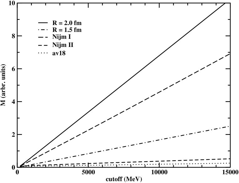
Figure 4: Cutoff ($\zeta$) dependence of the loop matrix element (21) for various wave functions as indicated. Two chiral wave functions with different matching radii $R$ were used, as well as some low-$\chi^{2}$ potential models.

In the context of pionic and electromagnetic processes in the two-nucleon system the pion-production reactions we are considering here are special. In all of the other reactions that we are aware of the operators occurring at low order in the chiral expansion diverge much less rapidly as $r\rightarrow 0$ than the $\frac{1}{r^{5}}$ of Eq. (24). In consequence the matrix elements of these operators do not have the sensitivity to the short-distance piece of the $NN$ wave function seen in Fig. 4. For an elegant demonstration of this in the context of pion-deuteron scattering, see Ref. NH05 .

The linear divergence of Eq. (24) (or Fig. 4) is removed by introducing a short-distance operator:

$$\mathcal{A}_{\rm ct}(\tilde{{\bf p}})\equiv\frac{1}{2}(\mbox{\boldmath${\sigma}$}_{1}+\mbox{\boldmath${\sigma}$}_{2})\cdot\tilde{\bf p}(i\tau_{1}^{a}-i\tau_{2}^{a})\frac{\tilde{d}_{0}(\zeta)}{Mf_{\pi}^{3}},$$ (25)

where $\tilde{d}_{0}(\zeta)$ is a dimensionless, cutoff-dependent constant. The operator (25) does not come from any term present in the original Lagrangian of Cohen , but such a contribution is required here because cutoff regularization is employed to compute the matrix element (21).

The operator (25) was not included in the analysis of Cohen et al. Cohen because the pion does not couple derivatively (or via powers of the pion mass) in $\mathcal{A}_{\rm ct}$, and therefore this operator cannot be derived from the Lagrangian of $\chi$PT. The analysis of Ref. Cohen uses that Lagrangian, together with naive dimensional analysis (NDA), to order all of the pion-production operators that are consistent with QCD’s chiral symmetry and the pattern of its breaking. In this case the regulator we have used when Fourier transforming the loop amplitude (16) breaks the chiral symmetry invoked when NDA was applied by Cohen et al. Cohen . Therefore we expect to have to add extra operators which break the symmetry in the same way as the regulator. Including such terms allows us to write down a renormalized amplitude that respects the symmetry—even though neither the loops or counterterm individually do. The term (25) must be included in our calculation, in spite of the fact that it violates chiral symmetry, so that it can cancel the chiral-symmetry-violating divergence (24) that is proportional to the cutoff $\zeta$.

Calculating the matrix element of $\mathcal{A}_{\rm ct}$ in $r$-space, we find [via Eq. (21)]

$$\mathcal{M}_{\rm ct}=-\mbox{\boldmath${\epsilon}$}_{d}^{\dagger}\cdot(\mbox{\boldmath${\widehat{\bf p}}$}\times\mbox{\boldmath${\epsilon}$}_{np})\frac{6\tilde{d}_{0}(\zeta)}{Mf_{\pi}^{3}}\sqrt{2E_{d}}\kappa_{0}\kappa_{1},$$ (26)

where $\mbox{\boldmath${\epsilon}$}_{np}$ is the polarization vector of the spin-1 nucleon pair and the Fourier transform creates a $\delta^{(3)}({\bf r})$ which picks up properties of the wave functions at the origin only. This can be evaluated without any regularization. It should come as no surprise that the expression (26) also does not vanish in the chiral limit. Of course, one can always choose the value of $\tilde{d}_{0}$ such that the sum of matrix elements for the loops and the counterterm vanishes in the limit $m_{\pi}\rightarrow 0$. However, since we are interested in pions with observed masses, we choose to extract $\tilde{d}_{0}(\zeta)$ at the physical threshold. This is to say, we fix the value of $\tilde{d}_{0}(\zeta)$ by fitting the experimental value of the threshold cross section Hutcheon . Given the behavior of the loop integral, $\tilde{d}_{0}$ will then run linearly with the cutoff $\zeta$. By construction the total matrix element will now reproduce the value of $\alpha$ from Ref. Hutcheon . Thus the renormalization not only removes the divergence in the $np\to d\pi^{0}$ matrix element that occurs at NLO, it also removes the wave-function dependence that we found in the LO result in Section III.

An alternative regularization of the matrix element of graphs 3(a) and 3(d) is provided by refraining from taking $\Lambda\rightarrow\infty$ directly after Fourier transforming, and instead keeping the regulator mass finite until after the matrix-element integral (21) has been performed. If we do this with a Gaussian regulator $\exp(-\tilde{p}^{2}/2\Lambda^{2})$ the loop matrix element becomes

$$\mathcal{M}_{\rm loops}=-\mbox{\boldmath${\epsilon}$}_{d}^{\dagger}\cdot(\mbox{\boldmath${\widehat{\bf p}}$}\times\mbox{\boldmath${\epsilon}$}_{np})\frac{g_{A}^{3}}{32f_{\pi}^{5}}\sqrt{\frac{2E_{d}}{\pi^{3}}}\Lambda^{5}\int dru(r)\tilde{I}(\Lambda r)v_{1}(r),$$ (27)

where $\tilde{I}(x)\equiv\frac{1}{2}[\frac{1}{x}-x+\sqrt{2}(\frac{1}{x^{2}}+2-x^{2})F(-x/\sqrt{2})]$ and $F(x)[=-F(-x)]$ is the Dawson integral

$$F(x)\equiv e^{-x^{2}}\int_{0}^{x}dte^{t^{2}}.$$ (28)

Surprisingly, in this procedure the coefficient of the linear divergence vanishes for local wave functions. But, it is still the case that the value found for the loop matrix element is sensitive to the short-distance physics. The result is strongly dependent on the wave function (see Fig. 5).

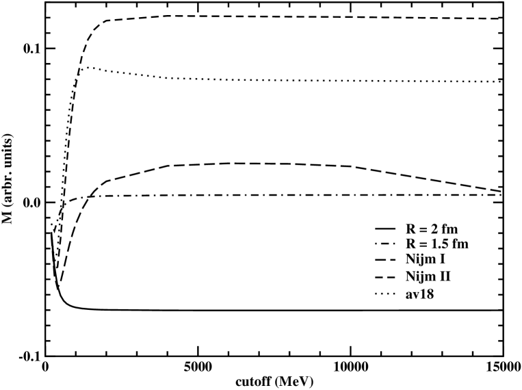
Figure 5: Single-regulator (Gaussian) cutoff ($\Lambda$) dependence of the loop matrix element for various wave functions as indicated.

The term linear in $\Lambda$ vanishes because there is a cancellation between the short- and long-distance (as separated by $1/\Lambda$) behavior of the integrand. If a function $F_{\Lambda}(\tilde{p})$ is used to regulate the Fourier transform then the divergent piece of the integral is [for fixed $\Lambda$ and using the $r<R_{\rm div}$ limits of $u(r)$ and $v_{1}(r)$]:

$$\int_{0}^{R_{\rm div}}dru(r)v_{1}(r)\,\frac{\partial}{\partial r}\int\frac{d^{3}\tilde{p}}{(2\pi)^{3}}\tilde{p}e^{i\tilde{\bf p}\cdot{\bf r}}F_{\Lambda}(\tilde{p})$$ (29)

$$= \frac{\kappa_{0}\kappa_{1}}{2\pi^{2}}\left[-r^{2}\frac{\partial^{2}}{\partial r^{2}}F_{\Lambda}(r)+3r\frac{\partial}{\partial r}F_{\Lambda}(r)-3F_{\Lambda}(r)\right]_{r=0}^{\infty}$$

$$\qquad\qquad-\quad\frac{\kappa_{0}\kappa_{1}}{2\pi^{2}}\left[-r^{2}\frac{\partial^{2}}{\partial r^{2}}F_{\Lambda}(r)+3r\frac{\partial}{\partial r}F_{\Lambda}(r)-3F_{\Lambda}(r)\right]_{r=R_{\rm div}}^{\infty}$$

$$\longrightarrow \frac{\kappa_{0}\kappa_{1}}{2\pi^{2}}\left[-r^{2}\frac{\partial^{2}}{\partial r^{2}}F_{\Lambda}(r)+3r\frac{\partial}{\partial r}F_{\Lambda}(r)-3F_{\Lambda}(r)\right]_{r=0}^{\infty}-\quad\frac{4\kappa_{0}\kappa_{1}}{\pi^{2}R_{\rm div}},$$

where we have taken the limit $\Lambda\to\infty$ in the second term on the last line, and $F_{\Lambda}(r)\equiv\int_{0}^{\infty}d\tilde{p}\sin(\tilde{p}r)F_{\Lambda}(\tilde{p})$. Any regulator for which the square bracket in the last line vanishes (a class which includes exponential and Gaussian regulators) produces a $\Lambda$-independent result in the $\Lambda\rightarrow\infty$ limit. Therefore the coefficient of the linear divergence is identically zero for such regulators. And indeed, Fig. 5 (calculated with a Gaussian cutoff) shows that calculations with a variety of wave functions produce flat behavior for 1–2 GeV $\lesssim\Lambda\lesssim 10$ GeV. (Qualitatively similar curves result if an exponential cutoff is used.)

For the local potentials, the flatness region persists at least up to $\approx 200$ GeV. Non-local potentials (e.g., Nijm I, Bonn models) start to deviate from flatness around 10 GeV, a hint of which is visible in Fig. 5. Their non-locality introduces additional high-momentum components that influences the wave functions at small $r$. These high-momentum components are neglected in the two-step procedure and there is no distinction between local and non-local potentials in Fig. 4.

The results of Fig. 5 confirm the prediction of Eq. (29). They do not show a divergence as the cutoff mass $\Lambda$ is taken to infinity. However, the matrix element remains non-vanishing in the chiral limit, and its value for $m_{\pi}=0$ will be determined by the high-energy mass scales $\kappa_{0}$, $\kappa_{1}$, and $R_{\rm div}$. These mass scales are related to the (implicit or explicit) scale-dependent regularizations carried out in obtaining the $NN$ wave functions we have used to calculate the matrix element. In order to remove this dependence on the (unphysical) wave-function regularization mass scale(s) we again introduce a short-distance operator of the structure (25). But this time we retain the regulator after Fourier transforming the operator to co-ordinate space, treating it in the same way as we did the loop-diagram operator when we obtained (27). The matrix element of the short-distance operator then reads:

$$\mathcal{M}_{\rm ct}=-2\mbox{\boldmath${\epsilon}$}_{d}^{\dagger}\cdot(\mbox{\boldmath${\widehat{\bf p}}$}\times\mbox{\boldmath${\epsilon}$}_{np})\frac{\tilde{d}_{0}(\Lambda)}{Mf_{\pi}^{3}}\frac{\sqrt{E_{d}}}{\pi}\Lambda^{5}\int rdru(r)e^{-\Lambda^{2}r^{2}/2}v_{1}(r).$$ (30)

We now include the short-distance operator (30) and adjust $\tilde{d}_{0}(\Lambda)$ such that the total matrix element squared gives $\bar{\alpha}_{0}=184$ $\mu$b. This yields the values for $\tilde{d}_{0}(\Lambda)$ shown in Table 2. The $\tilde{d}_{0}$’s shown there are, for most wave functions, quite rapidly varying with $\Lambda$. This is because the values given are for $\Lambda$ below the point where $\mathcal{M}_{\rm loop}$ becomes $\Lambda$ independent, see Fig. 5.

Table 2: Values for $\tilde{d}_{0}$ for various wave functions and cutoffs, using “one-step” regularization with Gaussian. For each $\Lambda$ there are two solutions, labeled (1) and (2).

	$\Lambda=400$ MeV		$\Lambda=800$ MeV		$\Lambda=1200$ MeV
potential	$\tilde{d}_{0}(1)$	$\tilde{d}_{0}(2)$	$\tilde{d}_{0}(1)$	$\tilde{d}_{0}(2)$	$\tilde{d}_{0}(1)$	$\tilde{d}_{0}(2)$
Nijm I	1.624	-0.0983	1.557	-0.125	1.669	-0.160
Nijm II	1.742	-0.199	2.629	-0.482	4.780	-1.079
av18	1.928	-0.2536	4.139	-0.857	10.138	-2.320
Bonn A	1.697	-0.1017	1.944	-0.194	2.365	-0.291
Bonn B	1.670	-0.1325	2.006	-0.257	2.678	-0.437
LO $\chi$PT(1.5 fm)	3.331	-0.7221	4.103	-0.935	4.368	-1.004
LO $\chi$PT(2 fm)	1.887	0.0072	1.502	0.0169	1.445	0.0179

For each $\Lambda$ there are two solutions for $\tilde{d}_{0}$ since we are solving a quadratic equation. Once $p$-waves are included in the calculation it should be possible to resolve this ambiguity with polarized data, e.g., $A_{y}$, which is available for $pp\to d\pi^{+}$ at low energies ppdpi . Such data fixes the relative phase between the $s$- and $p$-waves, provided the phase of the $p$-wave is known, see Eq. (4). We reiterate that, regardless of which value of $\tilde{d}_{0}$ turns out to be correct, the renormalization that is necessary at NLO in the threshold $np\to d\pi^{0}$ amplitude automatically eliminates the wave-function dependence that is present in the LO amplitude.

This procedure of regularizing using a Gaussian and keeping $\Lambda$ finite until after the matrix element is calculated seems more intuitively appealing and consistent than the “two-step” procedure introduced above. The fact that the term linearly proportional to the cutoff vanishes in such a “one-step” regularization also means that renormalization does not involve taking the difference of two large numbers.

Nevertheless, there remains a concern regarding the consistency of our use of two different regularization schemes: DR to compute the operators and cutoffs for the integrals we evaluate to obtain the matrix elements of those operators. Ideally the same regularization should be used for both pieces of our calculation. In this context we remind the reader that introducing a Pauli-Villars regulator (instead of DR) in the evaluation of the diagrams 3(a) and (d) results in a linear divergence appearing in the function $B(\tilde{p}^{2})$ [see Eq. (20)]. Therefore if a scale-dependent regulator is used to compute the loops of Fig. 3, a counterterm of the form (25) must be introduced already at the level of the operator, in order to facilitate renormalization of this linear divergence. Using DR—in which the renormalization of such linear divergences is performed implicitly by setting scale-less, linearly divergent integrals to zero—to compute $B(\tilde{p}^{2})$ postpones the necessity to introduce this counterterm. But it cannot be prolonged indefinitely if scale-dependent regulators are used to calculate the matrix element of the operator (16).

VI Energy dependence of $\bar{\alpha}$ at NLO

The NLO loops are proportional to $-\tilde{p}^{2}\sim M\omega_{q}$. Therefore, as at LO, $\chi$PT predicts that $\bar{\alpha}^{\prime}=\bar{\alpha}_{0}$ for the PWIA piece of the amplitude. The advantage at NLO is that short-range pion-production operators are included, which helps ameliorate the mismatch between the initial- and final-state momenta. Of course, $\alpha$ is now correctly reproduced, since the counterterm values given in Table 2 are found by adjusting $\bar{\alpha}_{0}$ to the experimental $184$ $\mu$b. Calculating the energy dependence of the reduced $s$-wave cross section and fitting it to $\bar{\alpha}=\bar{\alpha}_{0}+\bar{\alpha}^{\prime}\eta^{2}$ for various $\Lambda$’s, gives the values of Table 3. (For cutoffs above $\sim 1$ GeV the calculation becomes independent of $\Lambda$.)

Table 3: Values for $\bar{\alpha}^{\prime}$ (in $\mu$b) for various potentials, using counterterm values extracted for different $\Lambda$. The calculation is done for both $\tilde{d}_{0}$ solutions $(1)$ and $(2)$.

	$\Lambda=400$ MeV		$\Lambda=800$ MeV		$\Lambda=1200$ MeV
potential	$\bar{\alpha}^{\prime}(1)$	$\bar{\alpha}^{\prime}(2)$	$\bar{\alpha}^{\prime}(1)$	$\bar{\alpha}^{\prime}(2)$	$\bar{\alpha}^{\prime}(1)$	$\bar{\alpha}^{\prime}(2)$
Nijm I	29	-61	98	-53	108	-52
Nijm II	54	-78	144	-62	169	-59
av18	28	-84	102	-72	121	-69
Bonn A	14	-66	78	-59	87	-57
Bonn B	20	-72	82	-64	92	-63
$R=1.5$ fm	777	205	1471	352	1637	383
$R=2.0$ fm	277	93	434	103	466	104

Regardless of which choice we make for $\tilde{d}_{0}$, the chiral wave functions give results for $\bar{\alpha}^{\prime}$ that deviate considerably from the potential models and from each other, which might seem to be a disconcerting result. However, this deviation presumably comes from our neglecting TPEs, which seem to play an important role in processes at this momentum transfer. Our chiral wave functions, especially the one with $R=1.5$ fm, give a poor description of physics at $r<2$ fm. With this in mind we conclude that the range of NLO predictions for the two solutions is:

$$\bar{\alpha}^{\prime}(1) = 149\pm 41~{}\mu{\rm b},$$ (31)

$$\bar{\alpha}^{\prime}(2) = -60\pm 8~{}\mu{\rm b}.$$ (32)

The fact that (in either case) $\bar{\alpha}^{\prime}\neq\bar{\alpha}_{0}$ can be attributed almost entirely to distortions in the initial state, since higher-order ${\bf q}$ dependence in the amplitudes is a much smaller effect.

In fact, using the first $\tilde{d}_{0}$ value yields $\bar{\alpha}^{\prime}$s in reasonable accord with the PWIA ansatz $\bar{\alpha}^{\prime}\sim\bar{\alpha}_{0}$. If, on the other hand, the second solution is chosen, the NLO prediction for $\bar{\alpha}^{\prime}$ has only a very small shift from the LO result (15). Because of this convergence, we favor the second solution. The chiral series for $\bar{\alpha}^{\prime}$ seems to be behaving well, so we anticipate that higher-order corrections to the prediction (32) are $\lesssim 15$%. Once the $p$-waves have been calculated this result can be tested by comparison with, e.g., the analyzing power.

In any case, the results of Table 3 indicate that some of the experimental $\beta$ does arise from the energy dependence of the $s$-wave pion-production amplitude. However, $p$-wave pion production gives the greater part of the observed number.

VII Conclusions

We have calculated the $s$-wave cross section for $np\to d\pi^{0}$ (or, equivalently, the Coulomb-corrected $pp\to d\pi^{+}$), using chiral perturbation theory to NLO. We find that the dimensionally regularized NLO pion loops give a divergent result when they are sandwiched between wave functions, violating chiral-symmetry constraints. Thus the matrix element itself needs to be regularized. The variation with cutoff of this matrix element depends on the choice of regularization procedure. Regardless of the particular procedure chosen, a short-distance operator is needed to renormalize the theory. Matrix elements of both the loops alone and the short-distance operator alone are dependent on short-range physics, i.e., they display a strong variation with choice of wave function. However, by construction, their sum is cutoff independent at the pion-production threshold. A similar sensitivity to short-range physics has been observed in a calculation of $pp\to pp\pi^{0}$ Andoetal .

Therefore it is not immediately apparent that $\chi$PT can make more than a leading-order prediction for the threshold amplitude in $np\rightarrow d\pi^{0}$. This prediction has a modest wave-function dependence, but, being a LO result, is only accurate at the $\pm 40$% level. However, $\chi$PT does predict the energy-dependence of the $s$-wave pion-production operator. With an appropriate choice of the counterterm, this prediction is very little changed by NLO corrections. Pions produced in a relative $p$-wave are expected to give the remainder of the (non-trivial) energy-dependence of the near-threshold $np\rightarrow d\pi^{0}$ cross section. Understanding charge-independent $p$-wave pion production near threshold is also critical to an interpretation of the TRIUMF result for $A_{\rm fb}(np\to d\pi^{0})$, and so we are currently working on a calculation of the amplitude for $p$-wave pion production in $np\rightarrow d\pi^{0}$.

Note: Immediately before submitting this paper we became aware of an ongoing study by Lensky et al. Le05 . They propose a solution to the difficulty with the NLO pion-production operator we have identified here. This solution involves a careful treatment of the two-nucleon-reducible and two-nucleon-irreducible pieces obtained when the leading-order mechanism depicted in Fig. 2(a) is sandwiched between $NN$ wave functions. Presumably this also leads to a different prediction for the energy dependence of the NLO $s$-wave $np\rightarrow d\pi^{0}$ cross section.

- [1] See D. S. Koltun and A. Reitan, Phys. Rev. 141, 1413 (1966) for a treatment which does not use current algebra. But current algebra can be used to compute the phenomenological constants used in this work. For a recent summary see Ref. [18].
- [2] M. E. Schillaci, R. R. Silbar and J. E. Young, Phys. Rev. Lett. 21, 711 (1968); ibid. 1030 (E); Phys. Rev. 179, 1539 (1969).
- [3] S. Weinberg, Physica A 96, 327 (1979).
- [4] V. Bernard, N. Kaiser, and U.-G. Meißner, Int. J. Mod. Phys. E 4, 193 (1995).
- [5] S. Weinberg, Phys. Lett. B 251, 288 (1990); Nucl. Phys. B 363, 3 (1991).
- [6] C. Ordóñez and U. van Kolck, Phys. Lett. B 291, 459 (1992); C. Ordóñez, L. Ray, and U. van Kolck, Phys. Rev. C 53, 2086 (1996).
- [7] E. Epelbaum, W. Glöckle, and U.-G. Meißner, Nucl. Phys. A 671, 295 (2000); 747, 362 (2005); E. Epelbaum, [arXiv:nucl-th/0509032].
- [8] C. A. da Rocha, G. A. Miller and U. van Kolck, Phys. Rev. C 61, 034613 (2000).
- [9] C. Hanhart, J. Haidenbauer, O. Krehl, and J. Speth, Phys. Rev. C 61, 064008 (2000).
- [10] V. Malafaia, M. T. Peña, Ch. Elster, and J. Adam, Jr., [arXiv:nucl-th/0511038].
- [11] H. O. Meyer et al., Phys. Rev. Lett. 65, 2846 (1990); Nucl. Phys. A 539, 633 (1992); Phys. Rev. Lett. 81, 3096 (1998); 83, 5439 (1999).
- [12] A. Bondar et al., Phys. Lett. B 356, 8 (1995).
- [13] G. A. Miller and P. U. Sauer, Phys. Rev. C 44, R1725 (1991).
- [14] T.-S. H. Lee and D. O. Riska, Phys. Rev. Lett. 70, 2237 (1993).
- [15] C. J. Horowitz, H. O. Meyer, and D. K. Griegel, Phys. Rev. C 49, 1337 (1994).
- [16] E. Hernández and E. Oset, Phys. Lett. B 350, 158 (1995).
- [17] T. D. Cohen, J. L. Friar, G. A. Miller, and U. van Kolck, Phys. Rev. C 53, 2661 (1996).
- [18] B. Y. Park, F. Myhrer, J. R. Morones, T. Meissner and K. Kubodera, Phys. Rev. C 53, 1519 (1996).
- [19] T. Sato, T.-S. H. Lee, F. Myhrer, and K. Kubodera, Phys. Rev. C 56, 1246 (1997).
- [20] V. Dmitrašinović, K. Kubodera, F. Myhrer, and T. Sato, Phys. Lett. B 465, 43 (1999).
- [21] U. van Kolck, G. A. Miller and D. O. Riska, Phys. Lett. B 388, 679 (1996).
- [22] H. O. Meyer et al., Phys. Rev. C 63, 064002 (2001).
- [23] C. Hanhart, Phys. Rep. 397, 155 (2004).
- [24] C. Hanhart, U. van Kolck, and G. A. Miller, Phys. Rev. Lett. 85, 2905 (2000).
- [25] D. A. Hutcheon et al., Phys. Rev. Lett. 64, 176 (1990); Nucl. Phys. A 535, 618 (1991).
- [26] B. G. Ritchie, R. C. Minehart, T. D. Averett, G. S. Blanpied, K. Giovanetti, B. M. Preedom, D. Rothenberger, L. C. Smith, and J. R. Tinsley, Phys. Rev. Lett. 66, 568 (1991); B. G. Ritchie, T. D. Averett, D. Rothenberger, J. R. Tinsley, R. C. Minehart, K. Giovanetti, L. C. Smith, G. S. Blanpied, and B. M. Preedom, Phys. Rev. C 47, 21 (1993).
- [27] P. Heimberg et al., Phys. Rev. Lett. 77, 1012 (1996).
- [28] M. Drochner et al., Nucl. Phys. A 643, 55 (1998).
- [29] C. J. Horowitz, Phys. Rev. C 48, 2920 (1993).
- [30] J. A. Niskanen, Phys. Rev. C 53, C526 (1996).
- [31] A. K. Opper et al., Phys. Rev. Lett. 91, 212302 (2003).
- [32] E. J. Stephenson et al., Phys. Rev. Lett. 91, 142302 (2003).
- [33] U. van Kolck, J. A. Niskanen, and G. A. Miller, Phys. Lett. B 493, 65 (2000).
- [34] A. Gårdestig, C. J. Horowitz, A. Nogga, A. C. Fonseca, C. Hanhart, G. A. Miller, J. A. Niskanen, and U. van Kolck, Phys. Rev. C, 69, 044606 (2004).
- [35] E. Korkmaz, Jin Li, D. A. Hutcheon, R. Abegg, J. B. Elliott, L. G. Greeniaus, D. J. Mack, C. A. Miller, and N. L. Rodning, Nucl. Phys. A 535, 637 (1991).
- [36] S. R. Beane, P. F. Bedaque, W. C. Haxton, D. R. Phillips, and M. J. Savage, in Encyclopedia of Analytic QCD, At the Frontier of Particle Physics, vol. 1, 133-269, edited by M. Shifman (World Scientific, Singapore, 2001).
- [37] P. F. Bedaque and U. van Kolck, Ann. Rev. Nucl. Part. Sci. 52, 339 (2002).
- [38] D. R. Phillips, J. Phys. G 31, S1263 (2005).
- [39] C. Hanhart and N. Kaiser, Phys. Rev. C 66, 054005 (2002).
- [40] D. R. Phillips and T. D. Cohen, Nucl. Phys. A 668, 45 (2000).
- [41] A. Gårdestig and D. R. Phillips, Phys. Rev. C (in press); [arXiv:nucl-th/0501049].
- [42] V. G. J. Stoks, R. A. M. Klomp, M. C. M. Rentmeester, and J. J. de Swart, Phys. Rev. C 48, 792 (1993); http://nn-online.org
- [43] V. Stoks, R. Timmermans, and J. J. de Swart, Phys. Rev. C 47, 512 (1993).
- [44] M. C. M. Rentmeester, R. G. E. Timmermans, J. L. Friar, and J. J. de Swart, Phys. Rev. Lett. 82, 4992 (1999).
- [45] D. R. Entem and R. Machleidt, Phys. Rev. C 68, 041001(R) (2003);
- [46] V. G. J. Stoks, R. A. M. Klomp, C. P. F. Terheggen, and J. J. de Swart, Phys. Rev. C 49, 2950 (1994).
- [47] R. B. Wiringa, V. G. J. Stoks, and R. Schiavilla, Phys. Rev. C 51, 38 (1995).
- [48] T. S. Park, K. Kubodera, D. P. Min and M. Rho, Nucl. Phys. A 646, 83 (1999) [arXiv:nucl-th/9807054].
- [49] S. R. Beane, P. F. Bedaque, M. J. Savage and U. van Kolck, Nucl. Phys. A 700, 377 (2002) [arXiv:nucl-th/0104030].
- [50] A. Nogga, R. G. E. Timmermans, and U. van Kolck, [arXiv:nucl-th/0506005].
- [51] R. Machleidt, K. Holinde and C. Elster, Phys. Rep. 149, 1 (1987).
- [52] V. Bernard, N. Kaiser and U. G. Meissner, Eur. Phys. J. A 4, 259 (1999).
- [53] A. Nogga and C. Hanhart, arXiv:nucl-th/0511011.
- [54] S. Ando, T.-S. Park, and D.-P. Min, Phys. Lett. B 509, 253 (2001).
- [55] V. Lensky, V. Baru, J. Haidenbauer, C. Hanhart, A. Kudryavtsev, and U.-G, Meißner, [arXiv:nucl-th/0511054].