Exactly Solvable Models: The Road Towards a Rigorous Treatment of Phase Transitions in Finite Systems
Abstract
We discuss exact analytical solutions of a variety of statistical models recently obtained for finite systems by a novel powerful mathematical method, the Laplace-Fourier transform. Among them are a constrained version of the statistical multifragmentation model, the Gas of Bags Model and the Hills and Dales Model of surface partition. Thus, the Laplace-Fourier transform allows one to study the nuclear matter equation of state, the equation of state of hadronic and quark gluon matter and surface partitions on the same footing. A complete analysis of the isobaric partition singularities of these models is done for finite systems. The developed formalism allows us, for the first time, to exactly define the finite volume analogs of gaseous, liquid and mixed phases of these models from the first principles of statistical mechanics and demonstrate the pitfalls of earlier works. The found solutions may be used for building up a new theoretical apparatus to rigorously study phase transitions in finite systems. The strategic directions of future research opened by these exact results are also discussed.
Keywords:
Laplace-Fourier transform, statistical multifragmentation model, gas of bags model, phase transitions in finite systems:
25.70. Pq, 21.65.+f, 24.10. PaThere is always a sufficient amount of facts. Imagination is what we lack.
D. I. Blokhintsev
1 I. Theoretical Description of Phase Transitions in Finite Systems
A rigorous theory of critical phenomena in finite systems was not built up to now. However, the experimental studies of phase transitions (PTs) in some systems demand the formulation of such a theory. In particular, the investigations of the nuclear liquid-gas PT Bondorf:95 ; Gross:97 ; Moretto:97 require the development of theoretical approaches which would allow us to study the critical phenomena without going into the thermodynamic limit ( is the volume of the system) because such a limit does not exist due the long range Coulomb interaction. Therefore, there is a great need in the theoretical approaches which may shed light on the “internal mechanism” of how the PTs happen in finite systems.
The general situation in the theory of critical phenomena for finite (small) systems is not very optimistic at the moment because theoretical progress in this field has been slow. It is well known that the mathematical theory of phase transitions was worked out by T. D. Lee and C. N. Yang LeeYang . Unfortunately, there is no direct generic relation between the physical observables and zeros of the grand canonical partition in a complex fugacity plane. Therefore, we know very well what are the gaseous phase and liquid at infinite volumes: mixture of fragments of all sizes and ocean, respectively. This is known both for pure phases and for their mixture, but, despite some limited success Chomaz:03 , this general approach is not useful for the specific problems of critical phenomena in finite systems (see Sect. VIII below).
The tremendous complexity of critical phenomena in finite systems prevented their systematic and rigorous theoretical study. For instance, even the best formulation of the statistical mechanics and thermodynamics of finite systems by Hill Hill is not rigorous while discussing PTs. As a result, the absence of a well established definition of the liquid and mixed phase for finite volumes delays the progress of several related fields, including the theoretical and experimental searches for the reliable signals of several PTs which are expected to exist in strongly interacting matter. Therefore, the task of highest priority of the theory of critical phenomena is to define the finite volume analogs of phases from first principles of statistical mechanics. At present it is unclear whether such definitions can be made for a general case, but it turns out that such finite volume definitions can be formulated for a variety of realistic nonclassical (= non mean-field) statistical models which are successfully used in nuclear multifragmentation and in relativistic heavy collsisions.
About 25 years ago, when the theoretical foundations of nuclear multifragmentation were established, there was an illusion that the theoretical basis is simple and clear and, therefore, we need only the data and models which will describe them. The analysis of finite volume systems has proven to be very difficult. However, there was a clear way out of troubles by making numerical codes that are able to describe the data. This is, of course, a common way to handle such problems and there were many successes achieved in this way Bondorf:95 ; Gross:97 ; Moretto:97 ; Randrup:04 . However, there is another side of the coin which tells us that our understanding did not change much since then. This is so because the numerical simulations of this level do not provide us with any proof. At best they just demonstrate something. With time the number of codes increased, but the common theoretical approach was not developed. This led to a bitter result - there are many good guesses in the nuclear multifragmentation community, but, unfortunately, little analytical work to back up these expectations. As a result the absence of a firm theoretical ground led to formulation of such highly speculative “signals” of the nuclear liquid-vapor PT as negative heat capacity Negheat:1 ; Negheat:2 , bimodality Bimodality:1 , which later on were disproved, in Refs Negheat:3 and Bimodality:2 , respectively.
Thus, there is a paradoxic situation: there are many experimental data and facts, but there is no a single theoretical approach which is able to describe them. Similar to the searches for quark-gluon plasma (QGP) QM:04 there is lack of a firm and rigorous theoretical approach to describe phase transitions in finite systems.
However, our understanding of the multifragmentation phenomenon Bondorf:95 ; Gross:97 ; Moretto:97 was improved recently, when an exact analytical solution of a simplified version of the statistical multifragmentation model (SMM) Gupta:98 ; Gupta:99 was found in Refs. Bugaev:00 ; Bugaev:01 . These analytical results not only allowed us to understand the important role of the Fisher exponent on the phase structure of the nuclear liquid-gas PT and the properties of its (tri)critical point, but to calculate the critical indices of the SMM Reuter:01 as functions of index . The determination of the simplified SMM exponents allowed us to show explicitly Reuter:01 that, in contrast to expectations, the scaling relations for critical indices of the SMM differ from the corresponding relations of a well known Fisher droplet model (FDM) Fisher:67 . This exact analytical solution allowed us to predict a narrow range of values, , which, in contrast to FDM value , is consistent with ISiS Collaboration data ISIS and EOS Collaboration data EOS:00 . This finding is not only of a principal theoretical importance, since it allows one to find out the universality class of the nuclear liquid-gas phase transition, if index can be determined from experimental mass distribution of fragments, but also it enhanced a great activity in extracting the value of exponent from the data Karnaukhov:tau .
It is necessary to stress that such results in principle cannot be obtained either within the widely used mean-filed approach or numerically. This is the reason why exactly solvable models with phase transitions play a special role in statistical mechanics - they are the benchmarks of our understanding of critical phenomena that occur in more complicated substances. They are our theoretical laboratories, where we can study the most fundamental problems of critical phenomena which cannot be studied elsewhere. Their great advantage compared to other methods is that they provide us with the information obtained directly from the first principles of statistical mechanics being unspoiled by mean-field or other simplifying approximations without which the analytical analysis is usually impossible. On the other hand an exact analytical solution gives the physical picture of PT, which cannot be obtained by numerical evaluation. Therefore, one can expect that an extension of the exact analytical solutions to finite systems may provide us with the ultimate and reliable experimental signals of the nuclear liquid-vapor PT which are established on a firm theoretical ground of statistical mechanics. This, however, is a very difficult general task of the critical phenomena theory in finite systems.
Fortunately, we do not need to solve this very general task, but to find its solution for a specific problem of nuclear liquid-gas PT, which is less complicated and more realistic. In this case the straightforward way is to start from a few statistical models, like FDM and/or SMM, which are successful in describing the most of the experimental data. A systematic study of the various modifications of the FDM for finite volumes was performed by Moretto and collaborators Elliott:05wci and it led to a discovery of thermal reducibility of the fragment charge spectra Moretto:97 , to a determination of a quantitative liquid-vapor phase diagram containing the coexistence line up to critical temperature for small systems Elliott:02 ; Elliott:03 , to the generalization of the FDM for finite systems and to a formulation of the complement concept Precomplement ; Complement which allows one to account for finite size effects of (small) liquid drop on the properties of its vapor. However, such a systematic analysis for the SMM was not possible until recently, when its finite volume analytical solution was found in Bugaev:04a .
An invention of a new powerful mathematical method Bugaev:04a , the Laplace-Fourier transform, is a major theoretical breakthrough in the statistical mechanics of finite systems of the last decade because it allowed us to solve exactly not only the simplified SMM for finite volumes Bugaev:04a , but also a variety of statistical surface partitions for finite clusters Bugaev:04b and to find out their surface entropy and to shed light on a source of the Fisher exponent . It was shown Bugaev:04a that for finite volumes the analysis of the grand canonical partition (GCP) of the simplified SMM is reduced to the analysis of the simple poles of the corresponding isobaric partition, obtained as a Laplace-Fourier transform of the GCP. Such a representation of the GCP allows one not only to show from first principles that for finite systems there exist the complex values of the effective chemical potential, but to define the finite volume analogs of phases straightforwardly. Moreover, this method allows one to include into consideration all complicated features of the interaction (including the Coulomb one) which have been neglected in the simplified SMM because it was originally formulated for infinite nuclear matter. Consequently, the Laplace-Fourier transform method opens a principally new possibility to study the nuclear liquid-gas phase transition directly from the partition of finite system without taking its thermodynamic limit. Now this method is also applied Bugaev:05 to the finite volume formulation of the Gas of Bags Model (GBM) Goren:81 which is used to describe the PT between the hadronic matter and QGP. Thus, the Laplace-Fourier transform method not only gives an analytical solution for a variety of statistical models with PTs in finite volumes, but provides us with a common framework for several critical phenomena in strongly interacting matter. Therefore, it turns out that further applications and developments of this method are very promising and important not only for the nuclear multifragmentation community, but for several communities studying PTs in finite systems because this method may provide them with the firm theoretical foundations and a common theoretical language.
It is necessary to remember that further progress of this approach and its extension to other communities cannot be successfully achieved without new theoretical ideas about formalism it-self and its applications to the data measured in low and high energy nuclear collisions. Both of these require essential and coherent efforts of two or three theoretical groups working on the theory of PTs in finite systems, which, according to our best knowledge, do not exist at the moment either in multifragmentation community or elsewhere. Therefore, the second task of highest priority is to attract young and promising theoretical students to these theoretical problems and create the necessary manpower to solve the up coming problems. Otherwise the negative consequences of a complete dominance of experimental groups and numerical codes will never be overcome and a good chance to build up a common theoretical apparatus for a few PTs will be lost forever. If this will be the case, then an essential part of the nuclear physics associated with nuclear multifragmentation will have no chance to survive in the next years.
Therefore, the first necessary step to resolve these two tasks of highest priority is to formulate the up to day achievements of the exactly solvable models and to discuss the strategy for their further developments and improvements along with their possible impact on transport and hydrodynamic approaches. For these reasons the paper is organized as follows: in Sect. II we formulate the simplified SMM and present its analytical solution in thermodynamic limit; in Sect. III we discuss the necessary conditions for PT of given order and their relation to the singularities of the isobaric partition and apply these findings to the simplified SMM; Sect. IV is devoted to the SMM critical indices as the functions of Fisher exponent and their scaling relations; the Laplace-Fourier transform method is presented in Sect. V along with an exact analytical solution of the simplified SMM which has a constraint on the size of largest fragment, whereas the analysis of its isobaric partition singularities and the meaning of the complex values of free energy are given in Sect. VI; Sect. VII and VIII are devoted to the discussion of the case without PT and with it, respectively; at the end of Sect. VIII there is a discussion of the Chomaz and Gulminelli’s approach to bimodality Chomaz:03 ; in Sect. IX we discuss the finite volume modifications of the Gas of Bags, i.e. the statistical model describing the PT between hadrons and QGP, whereas in Sect. X we formulate the Hills and Dales Model for the surface partition and present the limit of the vanishing amplitudes of deformations; and, finally, in Sect. XI we discuss the strategy of future research which is necessary to build up a truly microscopic kinetics of phase transitions in finite systems.
2 II. Statistical Multifragmentation in Thermodynamic Limit
The system states in the SMM are specified by the multiplicity sets () of -nucleon fragments. The partition function of a single fragment with nucleons is Bondorf:95 : , where ( is the total number of nucleons in the system), and are, respectively, the volume and the temperature of the system, is the nucleon mass. The first two factors on the right hand side (r.h.s.) of the single fragment partition originate from the non-relativistic thermal motion and the last factor, , represents the intrinsic partition function of the -nucleon fragment. Therefore, the function is a phase space density of the k-nucleon fragment. For (nucleon) we take (4 internal spin-isospin states) and for fragments with we use the expression motivated by the liquid drop model (see details in Ref. Bondorf:95 ): with fragment free energy
| (1) |
with . Here MeV is the bulk binding energy per nucleon. is the contribution of the excited states taken in the Fermi-gas approximation ( MeV). is the temperature dependent surface tension parameterized in the following relation: with MeV and MeV ( at ). The last contribution in Eq. (1) involves the famous Fisher’s term with dimensionless parameter .
It is necessary to stress that the SMM parametrization of the surface tension coefficient is not a unique one. For instance, the FDM successfully employs another one As we shall see in Sect. IV the temperature dependence of the surface tension coefficient in the vicinity of the critical point will define the critical indices of the model, but the following mathematical analysis of the SMM is general and is valid for an arbitrary function.
The canonical partition function (CPF) of nuclear fragments in the SMM has the following form:
| (2) |
In Eq. (2) the nuclear fragments are treated as point-like objects. However, these fragments have non-zero proper volumes and they should not overlap in the coordinate space. In the excluded volume (Van der Waals) approximation this is achieved by substituting the total volume in Eq. (2) by the free (available) volume , where ( fm-3 is the normal nuclear density). Therefore, the corrected CPF becomes: . The SMM defined by Eq. (2) was studied numerically in Refs. Gupta:98 ; Gupta:99 . This is a simplified version of the SMM, since the symmetry and Coulomb contributions are neglected. However, its investigation appears to be of principal importance for studies of the nuclear liquid-gas phase transition.
The calculation of is difficult due to the constraint . This difficulty can be partly avoided by evaluating the grand canonical partition (GCP)
| (3) |
where denotes a chemical potential. The calculation of is still rather difficult. The summation over sets in cannot be performed analytically because of additional -dependence in the free volume and the restriction . The presence of the theta-function in the GCP (3) guarantees that only configurations with positive value of the free volume are counted. However, similarly to the delta function restriction in Eq. (2), it makes again the calculation of (3) to be rather difficult. This problem was resolved Bugaev:00 ; Bugaev:01 by performing the Laplace transformation of . This introduces the so-called isobaric partition function (IP) Goren:81 :
| (4) | |||||
After changing the integration variable , the constraint of -function has disappeared. Then all were summed independently leading to the exponential function. Now the integration over in Eq. (4) can be done resulting in
| (5) |
where
| (6) |
Here we have introduced the shifted chemical potential . From the definition of pressure in the grand canonical ensemble it follows that, in the thermodynamic limit, the GCP of the system behaves as
| (7) |
An exponentially over increasing part of in the right-hand side of Eq. (7) generates the rightmost singularity of the function , because for the -integral for (4) diverges at its upper limit. Therefore, in the thermodynamic limit, the system pressure is defined by this rightmost singularity, , of IP (4):
| (8) |
Note that this simple connection of the rightmost -singularity of , Eq. (4), to the asymptotic, , behavior of , Eq. (7), is a general mathematical property of the Laplace transform. Due to this property the study of the system behavior in the thermodynamic limit can be reduced to the investigation of the singularities of .
3 III. Singularities of Isobaric Partition and Phase Transitions
The IP, Eq. (4), has two types of singularities: 1) the simple pole singularity defined by the equation
| (9) |
2) the singularity of the function it-self at the point where the coefficient in linear over terms in the exponent is equal to zero,
| (10) |
The simple pole singularity corresponds to the gaseous phase where pressure is determined by the equation
| (11) |
The singularity of the function (6) defines the liquid pressure
| (12) |
In the considered model the liquid phase is represented by an infinite fragment, i.e. it corresponds to the macroscopic population of the single mode . Here one can see the analogy with the Bose condensation where the macroscopic population of a single mode occurs in the momentum space.
In the -regions where the gas phase dominates (), while the liquid phase corresponds to . The liquid-gas phase transition occurs when two singularities coincide, i.e. . A schematic view of singular points is shown in Fig. 1a for , i.e. when . The two-phase coexistence region is therefore defined by the equation
| (13) |
One can easily see that is monotonously decreasing function of . The necessary condition for the phase transition is that this function remains finite in its singular point :
| (14) |
The convergence of is determined by and . At the condition (14) requires . Otherwise, and the simple pole singularity (9) is always the rightmost -singularity of (4) (see Fig. 1b). At , where , the considered system can exist only in the one-phase state. It will be shown below that for the condition (14) can be satisfied even at .


At the system undergoes the 1-st order phase transition across the line defined by Eq.(13). Its explicit form is given by the expression:
| (15) |
The points on the line correspond to the mixed phase states. First we consider the case because it is the standard SMM choice.
The baryonic density is found as and is given by the following formulae in the liquid and gas phases
| (16) |
respectively. Here the function is defined as
| (17) |


Due to the condition (13) this expression is simplified in the mixed phase:
| (18) |
This formula clearly shows that the bulk (free) energy acts in favor of the composite fragments, but the surface term favors single nucleons.
Since at the sum in Eq. (18) converges at any , is finite and according to Eq. (16) . Therefore, the baryonic density has a discontinuity across the line (15) for any . The discontinuities take place also for the energy and entropy densities. The phase diagram of the system in the -plane is shown in the left panel of Fig. 2. The line (15) corresponding to the mixed phase states is transformed into the finite region in the -plane. As usual, in this mixed phase region of the phase diagram the baryonic density and the energy density are superpositions of the corresponding densities of liquid and gas:
| (19) |
Here () is a fraction of the system volume occupied by the liquid inside the mixed phase, and the partial energy densities for can be found from the thermodynamic identity Bugaev:00 :
| (20) |
Inside the mixed phase at constant density the parameter has a specific temperature dependence shown in the left panel of Fig. 3: from an approximately constant value at small the function drops to zero in a narrow vicinity of the boundary separating the mixed phase and the pure gaseous phase. This corresponds to a fast change of the configurations from the state which is dominated by one infinite liquid fragment to the gaseous multifragment configurations. It happens inside the mixed phase without discontinuities in the thermodynamical functions.
An abrupt decrease of near this boundary causes a strong increase of the energy density as a function of temperature. This is evident from the middle panel of Fig. 3 which shows the caloric curves at different baryonic densities. One can clearly see a leveling of temperature at energies per nucleon between 10 and 20 MeV. As a consequence this leads to a sharp peak in the specific heat per nucleon at constant density, , presented in Fig. 3. A finite discontinuity of arises at the boundary between the mixed phase and the gaseous phase. This finite discontinuity is caused by the fact that , but at this boundary (see Fig. 3).
It should be emphasized that the energy density is continuous at the boundary of the mixed phase and the gaseous phase, hence the sharpness of the peak in is entirely due to the strong temperature dependence of near this boundary. Moreover, at any the maximum value of remains finite and the peak width in is nonzero in the thermodynamic limit considered in our study. This is in contradiction with the expectation of Refs. Gupta:98 ; Gupta:99 that an infinite peak of zero width will appear in in this limit. Also a comment about the so-called “boiling point” is appropriate here. This is a discontinuity in the energy density or, equivalently, a plateau in the temperature as a function of the excitation energy. Our analysis shows that this type of behavior indeed happens at constant pressure, but not at constant density! This is similar to the usual picture of a liquid-gas phase transition. In Refs. Gupta:98 ; Gupta:99 a rapid increase of the energy density as a function of temperature at fixed near the boundary of the mixed and gaseous phases (see the right panel of Fig. 3) was misinterpreted as a manifestation of the “boiling point”.
New possibilities appear at non-zero values of the parameter . At the qualitative picture remains the same as discussed above, although there are some quantitative changes. For the condition (14) is also satisfied at where . Therefore, the liquid-gas phase transition extends now to all temperatures. Its properties are, however, different for and for (see Fig. 2). If the gas density is always lower than as is finite. Therefore, the liquid-gas transition at remains the 1-st order phase transition with discontinuities of baryonic density, entropy and energy densities (right panel in Fig. 2) .


Middle panel: Temperature as a function of energy density per nucleon (caloric curve) is shown for fixed nucleon densities and . Note that the shape of the model caloric curves is very similar to the experimental finding Natowitz:02 , although our estimates for the excitation energy is somewhat larger due to oversimplified interaction. For a quantitative comparison between the simplified SMM the full SMM interaction should be accounted for.
Right panel: Specific heat per nucleon as a function of temperature at fixed nucleon density . The dashed line shows the finite discontinuity of at the boundary of the mixed and gaseous phases for .
4 IV. The Critical Indices and Scaling Relations of the SMM
The above results allow one to find the critical exponents and of the simplified SMM. These exponents describe the temperature dependence of the system near the critical point on the coexistence curve (13), where the effective chemical potential vanishes
| (23) | |||||
| (24) | |||||
| (25) |
where defines the order parameter, denotes the specific heat at fixed particle density and is the isothermal compressibility. The shape of the critical isotherm for is given by the critical index (the tilde indicates hereafter)
| (26) |
The calculation of and requires the specific heat . With the formula Ya:64
| (27) |
one obtains the specific heat on the PT curve by replacing the partial derivatives by the total ones Fi:70 . The latter can be done for every state inside or on the boundary of the mixed phase region. For the chemical potential one gets Here the asterisk indicates the condensation line () hereafter. Fixing one finds and, hence, obtains To calculate , and the behavior of the series
| (28) |
should be analyzed for small positive values of and . In the limit the function remains finite, if , and diverges otherwise. For this divergence is logarithmic. The case is analyzed in some details, since even in Fisher’s papers it was performed incorrectly.
With the substitution one can prove Reuter:01 that in the limit the series on the r. h. s. of (28) converges to an integral
| (29) |
The assumption is sufficient to guarantee the convergence of the integral at its lower limit. Using this representation, one finds the following general results Reuter:01
| (30) |
which allowed us to find out the critical indices of the SMM (see Table 1).
| SMM for | |||||
|---|---|---|---|---|---|
| SMM for | |||||
| FDM | N/A |
In the special case the well-known exponent inequalities proven for real gases by
| (31) | |||||
| (32) | |||||
| (33) |
are fulfilled exactly for any . (The corresponding exponent inequalities for magnetic systems are often called Rushbrooke’s, Griffiths’ and Widom’s inequalities, respectively.) For , Fisher’s and Griffiths’ exponent inequalities are fulfilled as inequalities and for they are not fulfilled. The contradiction to Fisher’s and Griffiths’ exponent inequalities in this last case is not surprising. This is due to the fact that in the present version of the SMM the critical isochore lies on the boundary of the mixed phase to the liquid. Therefore, in expression (2.13) in Ref. Fi:64 for the specific heat only the liquid phase contributes and, therefore, Fisher’s proof of Ref. Fi:64 following (2.13) cannot be applied for the SMM. Thus, the exponent inequalities (31) and (32) have to be modified for the SMM. Using results of Table 1, one finds the following scaling relations
| (34) |
Liberman’s exponent inequality (33) is fulfilled exactly for any choice of and .
Since the coexistence curve of the SMM is not symmetric with respect to , it is interesting with regard to the specific heat to consider the difference , following the suggestion of Ref. Fi:70 . Using Eq. (27) for gas and liquid and noting that , one obtains a specially defined index from the most divergent term for
| (37) |
Then it is for . Thus, approaching the critical point along any isochore within the mixed phase region except for the specific heat diverges for as defined by and remains finite for the isochore . This demonstrates the exceptional character of the critical isochore in this model.
In the special case that one finds for and for . Therefore, using instead of , the exponent inequalities (31) and (32) are fulfilled exactly if and or if and . In all other cases (31) and (32) are fulfilled as inequalities. Moreover, it can be shown that the SMM belongs to the universality class of real gases for and .
The comparison of the above derived formulae for the critical exponents of the SMM for with those obtained within the FDM (Eqs. 51-56 in Fisher:67 ) shows that these models belong to different universality classes (except for the singular case ).
Furthermore, one has to note that for and the critical exponents of the SMM coincide with those of the exactly solved one-dimensional FDM with non-zero droplet-volumes Fi:70 .
For the usual parameterization of the SMM Bondorf:95 one obtains with and the exponents
| (40) |
Thus, Fisher suggestion to use instead of allows one to “save” the exponential inequalities, however, it is not a final solution of the problem.
The critical indices of the nuclear liquid-gas PT were determined from the multifragmentation of gold nuclei Eos:94 and found to be close to those ones of real gases. The method used to extract the critical exponents and in Ref. Eos:94 was, however, found to have large uncertainties of about 25 per cents Bau:94 . Nevertheless, those results allow us to estimate the value of from the experimental values of the critical exponents of real gases taken with large error bars. Using the above results we generalized Reuter:01 the exponent relations of Ref. Fi:70
| (41) |
for arbitrary and . Then, one obtains with Hu , and the estimate . This demonstrates also that the value of is rather insensitive to the special choice of and , which leads to for the SMM. Theoretical values for and for Ising-like systems within the renormalized theory Zi:98 lead to the narrow range . The values of and indices for nuclear matter and percolation of two- and three-dimensional clusters are reviewed in Elliott:05wci .
There was a decent try to study the critical indices of the SMM numerically El:00 . The version V2 of Ref. El:00 corresponds precisely to our model with , and , but their results contradict to our analysis. Their results for version V3 of Ref. El:00 are in contradiction with our proof presented in Ref. Bugaev:00 . There it was shown that for non-vanishing surface energy (as in version V3) the critical point does not exist at all. The latter was found in El:00 for the finite system and the critical indices were analyzed. Such a strange result, on one hand, indicates that the numerical methods used in Ref. El:00 are not self-consistent, and, on the other hand, it shows an indispensable value of the analytical calculations, which can be used as a test problem for numerical algorithms.
It is widely believed that the effective value of defined as attains its minimum at the critical point (see references in EOS:00 ). This has been shown for the version of the FDM with the constraint of sufficiently small surface tension for Pan:83 and also can be seen easily for the SMM. Taking the SMM fragment distribution one finds
| (42) |
where the last step follows from the fact that the inequalities , become equalities at the critical point . Therefore, the SMM predicts that the minimal value of corresponds to the critical point.
In the E900 Au multifragmentation experiment ISIS the ISiS collaboration measured the dependence of upon the excitation energy and found the minimum value (Fig. 5 of Ref. ISIS ). Also the EOS collaboration EOS:00 performed an analysis of the minimum of on Au + C multifragmentation data. The fitted , plotted in Fig. 11.b of Ref. EOS:00 versus the fragment multiplicity, exhibits a minimum in the range . Both results contradict the original FDM Fisher:67 , but agree well with the above estimate of for real gases and for Ising-like systems in general.
5 V. Constrained SMM in Finite Volumes
Despite the great success, the application of the exact solution Bugaev:00 ; Bugaev:01 ; Reuter:01 to the description of experimental data is limited because this solution corresponds to an infinite system and due to that it cannot account for a more complicated interaction between nuclear fragments. Therefore, it was necessary to extend the exact solution Bugaev:00 ; Bugaev:01 ; Reuter:01 to finite volumes. It is clear that for the finite volume extension it is necessary to account for the finite size and geometrical shape of the largest fragments, when they are comparable with the system volume. For this one has to abandon the arbitrary size of largest fragment and consider the constrained SMM (CSMM) in which the largest fragment size is explicitly related to the volume of the system. Thus, the CSMM assumes a more strict constraint , where the size of the largest fragment cannot exceed the total volume of the system (the parameter is introduced for convenience). The case of the fixed size of the largest fragment, i.e. , analyzed numerically in Ref. CSMM is also included in our treatment. A similar restriction should be also applied to the upper limit of the product in all partitions , and introduced above (how to deal with the real values of , see later). Then the model with this constraint, the CSMM, cannot be solved by the Laplace transform method, because the volume integrals cannot be evaluated due to a complicated functional -dependence. However, the CSMM can be solved analytically with the help of the following identity Bugaev:04a
| (43) |
which is based on the Fourier representation of the Dirac -function. The representation (43) allows us to decouple the additional volume dependence and reduce it to the exponential one, which can be dealt by the usual Laplace transformation in the following sequence of steps
| (44) |
After changing the integration variable , the constraint of -function has disappeared. Then all were summed independently leading to the exponential function. Now the integration over in Eq. (5) can be straightforwardly done resulting in
| (45) |
where the function is defined as follows
| (46) |
As usual, in order to find the GCP by the inverse Laplace transformation, it is necessary to study the structure of singularities of the isobaric partition (46).
6 VI. Isobaric Partition Singularities at Finite Volumes
The isobaric partition (46) of the CSMM is, of course, more complicated than its SMM analog Bugaev:00 ; Bugaev:01 because for finite volumes the structure of singularities in the CSMM is much richer than in the SMM, and they match in the limit only. To see this let us first make the inverse Laplace transform:
| (47) | |||||
noindent where the contour -integral is reduced to the sum over the residues of all singular points with , since this contour in the complex -plane obeys the inequality . Now both remaining integrations in (47) can be done, and the GCP becomes
| (48) |
i.e. the double integral in (47) simply reduces to the substitution in the sum over singularities. This is a remarkable result which was formulated in Ref. Bugaev:04a as the following theorem: if the Laplace-Fourier image of the excluded volume GCP exists, then for any additional -dependence of or the GCP can be identically represented by Eq. (48).
The simple poles in (47) are defined by the equation
| (49) |
In contrast to the usual SMM Bugaev:00 ; Bugaev:01 the singularities are (i) are volume dependent functions, if is not constant, and (ii) they can have a non-zero imaginary part, but in this case there exist pairs of complex conjugate roots of (49) because the GCP is real.
Introducing the real and imaginary parts of , we can rewrite Eq. (49) as a system of coupled transcendental equations
| (50) | |||
| (51) |
where we have introduced the set of the effective chemical potentials with , and the reduced distributions and for convenience.
Consider the real root , first. For the real root exists for any and . Comparing with the expression for vapor pressure of the analytical SMM solution Bugaev:00 ; Bugaev:01 shows that is a constrained grand canonical pressure of the gas. As usual, for finite volumes the total mechanical pressure Hill ; Bugaev:04a differs from . Equation (51) shows that for the inequality never become the equality for all -values simultaneously. Then from Eq. (50) one obtains ()
| (52) |
where the second inequality (52) immediately follows from the first one. In other words, the gas singularity is always the rightmost one. This fact plays a decisive role in the thermodynamic limit .
The interpretation of the complex roots is less straightforward. According to Eq. (48), the GCP is a superposition of the states of different free energies . (Strictly speaking, has a meaning of the change of free energy, but we will use the traditional term for it.) For the free energies are complex. Therefore, is the density of free energy. The real part of the free energy density, , defines the significance of the state’s contribution to the partition: due to (52) the largest contribution always comes from the gaseous state and has the smallest real part of free energy density. As usual, the states which do not have the smallest value of the (real part of) free energy, i. e. , are thermodynamically metastable. For infinite volume they should not contribute unless they are infinitesimally close to , but for finite volumes their contribution to the GCP may be important.
As one sees from (50) and (51), the states of different free energies have different values of the effective chemical potential , which is not the case for infinite volume Bugaev:00 ; Bugaev:01 , where there exists a single value for the effective chemical potential. Thus, for finite the states which contribute to the GCP (48) are not in a true chemical equilibrium.
The meaning of the imaginary part of the free energy density becomes clear from (50) and (51) Bugaev:05csmm : as one can see from (50) the imaginary part effectively changes the number of degrees of freedom of each -nucleon fragment () contribution to the free energy density . It is clear, that the change of the effective number of degrees of freedom can occur virtually only and, if state is accompanied by some kind of equilibration process. Both of these statements become clear, if we recall that the statistical operator in statistical mechanics and the quantum mechanical convolution operator are related by the Wick rotation Feynmann . In other words, the inverse temperature can be considered as an imaginary time. Therefore, depending on the sign, the quantity that appears in the trigonometric functions of the equations (50) and (51) in front of the imaginary time can be regarded as the inverse decay/formation time of the metastable state which corresponds to the pole (for more details see next sections).
This interpretation of naturally explains the thermodynamic metastability of all states except the gaseous one: the metastable states can exist in the system only virtually because of their finite decay/formation time, whereas the gaseous state is stable because it has an infinite decay/formation time.
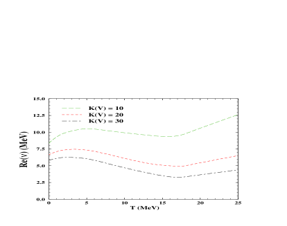
Right panel: Each curve separates the region of one real root of Eq. (49) (below the curve), three complex roots (at the curve) and four and more roots (above the curve) for three values of and the same parameters as in the left panel.
7 VII. No Phase Transition Case
It is instructive to treat the effective chemical potential as an independent variable instead of . In contrast to the infinite , where the upper limit defines the liquid phase singularity of the isobaric partition and gives the pressure of a liquid phase Bugaev:00 ; Bugaev:01 , for finite volumes and finite the effective chemical potential can be complex (with either sign for its real part) and its value defines the number and position of the imaginary roots in the complex plane. Positive and negative values of the effective chemical potential for finite systems were considered Elliott:01 within the Fisher droplet model, but, to our knowledge, its complex values have never been discussed. From the definition of the effective chemical potential it is evident that its complex values for finite systems exist only because of the excluded volume interaction, which is not taken into account in the Fisher droplet model Fisher:67 . However, a recent study of clusters of the Ising model within the framework of FDM (see the corresponding section in Ref. Elliott:05wci ) shows that the excluded volume correction improves essentially the description of the thermodynamic functions. Therefore, the next step is to consider the complex values of the effective chemical potential and free energy for the excluded volume correction of the Ising clusters on finite lattices.
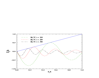
As it is seen from Fig. 1, the r.h.s. of Eq. (51) is the amplitude and frequency modulated sine-like function of dimensionless parameter . Therefore, depending on and values, there may exist no complex roots , a finite number of them, or an infinite number of them. In Fig. 1 we showed a special case which corresponds to exactly three roots of Eq. (49) for each value of : the real root () and two complex conjugate roots (). Since the r.h.s. of (51) is monotonously increasing function of , when the former is positive, it is possible to map the plane into regions of a fixed number of roots of Eq. (49). Each curve in Fig. 2 divides the plane into three parts: for -values below the curve there is only one real root (gaseous phase), for points on the curve there exist three roots, and above the curve there are four or more roots of Eq. (49).
For constant values of the number of terms in the r.h.s. of (51) does not depend on the volume and, consequently, in thermodynamic limit only the rightmost simple pole in the complex -plane survives out of a finite number of simple poles. According to the inequality (52), the real root is the rightmost singularity of isobaric partition (45). However, there is a possibility that the real parts of other roots become infinitesimally close to , when there is an infinite number of terms which contribute to the GCP (48).
Let us show now that even for an infinite number of simple poles in (48) only the real root survives in the limit . For this purpose consider the limit . In this limit the distance between the imaginary parts of the nearest roots remains finite even for infinite volume. Indeed, for the leading contribution to the r.h.s. of (51) corresponds to the harmonic with , and, consequently, an exponentially large amplitude of this term can be only compensated by a vanishing value of , i.e. with (hereafter we will analyze only the branch ), and, therefore, the corresponding decay/formation time is volume independent.
Keeping the leading term on the r.h.s. of (51) and solving for , one finds
| (53) | |||||
| (54) |
where in the last step we used Eq. (50) and condition . Since for all negative values of cannot contribute to the GCP (48), it is sufficient to analyze even values of which, according to (54), generate .
Since the inequality (52) can not be broken, a single possibility, when pole can contribute to the partition (48), corresponds to the case for some finite . Assuming this, we find for the same value of . Substituting these results into equation (50), one gets
| (55) |
The inequality (55) follows from the equation for and the fact that, even for equal leading terms in the sums above (with and even ), the difference between and is large due to the next to leading term , which is proportional to . Thus, we arrive at a contradiction with our assumption , and, consequently, it cannot be true. Therefore, for large volumes the real root always gives the main contribution to the GCP (48), and this is the only root that survives in the limit . Thus, we showed that the model with the fixed size of the largest fragment has no phase transition because there is a single singularity of the isobaric partition (45), which exists in thermodynamic limit.
8 VIII. Finite Volume Analogs of Phases
If monotonically grows with the volume, the situation is different. In this case for positive value of the leading exponent in the r.h.s. of (51) also corresponds to a largest fragment, i.e. to . Therefore, we can apply the same arguments which were used above for the case and derive similarly equations (53)–(54) for and . From it follows that, when increases, the number of simple poles in (47) also increases and the imaginary part of the closest to the real -axis poles becomes very small, i.e for , and, consequently, the associated decay/formation time grows with the volume of the system. Due to , the inequality (55) cannot be established for the poles with . Therefore, in contrast to the previous case, for large the simple poles with will be infinitesimally close to the real axis of the complex -plane.
From Eq. (54) it follows that
| (56) |
for and . Thus, we proved that for infinite volume the infinite number of simple poles moves toward the real -axis to the vicinity of liquid phase singularity of the isobaric partition Bugaev:00 ; Bugaev:01 and generates an essential singularity of function in (46) irrespective to the sign of the chemical potential . In addition, as we showed above, the states with become stable because they acquire infinitely large decay/formation time in the limit . Therefore, these states should be identified as a liquid phase for finite volumes as well.
Now it is clear that each curve in Fig. 2 is the finite volume analog of the phase boundary for a given value of : below the phase boundary there exists a gaseous phase, but at and above each curve there are states which can be identified with a finite volume analog of the mixed phase, and, finally, at there exists a liquid phase. When there is no phase transition, i.e. , the structure of simple poles is similar, but, first, the line which separates the gaseous states from the metastable states does not change with the volume, and, second, as shown above, the metastable states will never become stable. Therefore, a systematic study of the volume dependence of free energy (or pressure for very large ) along with the formation and decay times may be of a crucial importance for experimental studies of the nuclear liquid gas phase transition.
The above results demonstrate that, in contrast to Hill’s expectations Hill , the finite volume analog of the mixed phase does not consist just of two pure phases. The mixed phase for finite volumes consists of a stable gaseous phase and the set of metastable states which differ by the free energy. Moreover, the difference between the free energies of these states is not surface-like, as Hill assumed in his treatment Hill , but volume-like. Furthermore, according to Eqs. (50) and (51), each of these states consists of the same fragments, but with different weights. As seen above for the case , some fragments that belong to the states, in which the largest fragment is dominant, may, in principle, have negative weights (effective number of degrees of freedom) in the expression for (50). This can be understood easily because higher concentrations of large fragments can be achieved at the expense of the smaller fragments and is reflected in the corresponding change of the real part of the free energy . Therefore, the actual structure of the mixed phase at finite volumes is more complicated than was expected in earlier works.
The Hills’ ideas were developed further in Ref. Chomaz:03 , where the authors claimed to establish the one to one correspondence between the bimodal structure of the partition of measurable quantity known on average and the properties of the Lee-Yang zeros of this partition in the complex -plane. The starting point of Ref. Chomaz:03 is to postulate the partition and the probability of the following form
| (57) |
where is the partition sum of the ensemble of fixed values of the observable , and is the corresponding Lagrange multiplier. Then the authors of Ref. Chomaz:03 assume the existence of two maxima of the probability ( bimodality) and discuss their relation to the Lee-Yang zeros of in the complex -plane.
The CSMM gives us a unique opportunity to verify the Chomaz and Gulminelli idea on the bimodality behavior of using the first principle results. Let us use the equation (5) identifying the intensive variable with and extensive one with the available volume . The evaluation of the r.h.s. of (5) is very difficult in general, but for a special case, when the eigen volume is small this can be done analytically. Thus, approximating , we obtain the CSMM analog of the probability (57)
| (58) |
where we made the integration after applying the approximation for . Further evaluation of (58) requires to know all possible solutions of the average volume of the system (). It can be shown Bugaev:05csmm that for the gaseous domain (see the right panel of Fig. 4) there exist a single solution , whereas for the domain , which corresponds to a finite volume analog of the mixed phase, there are two solutions . In contrast to the expectations of Ref. Chomaz:03 , the probability (58)
| (59) |
has negative derivative for the whole domain of existence of the isobaric partition Bugaev:05csmm . This is true even for the domain in which, as we proved, there exists a finite analog of the mixed phase, i.e. for . Moreover, irrespective to the sign of the derivative , the probability (58) cannot be measured experimentally. Above it was rigorously proven that for any real the IP is defined on the real -axis only for , i.e. on the right hand side of the gaseous singularity : . However, as one can see from the equation (47), the “experimental” values belong to the other region of the complex -plane: .
Thus, it turns out that the suggestion of Ref. Chomaz:03 to analyze the probability (57) does not make any sense because, as we showed explicitly for the CSMM, it cannot be measured. It seems that the starting point of the Ref. Chomaz:03 approach, i.e. the assumption that the left equation (57) gives the most general form of the partition of finite system, is problematic. Indeed, comparing (56) with the analytical result (59), we see that for finite systems, in contrast to the major assumption of Ref. Chomaz:03 , the probability of the CSMM depends not only on the extensive variable , but also on the intensive variable , which makes unmeasurable the whole construct of Ref. Chomaz:03 . Consequently, the conclusions of Ref. Chomaz:03 on the relation between the bimodality and the phase transition existence are not general and have a limited range of validity. In addition, the absence of two maxima of the probability (59) automatically means the absence of back-banding of the equation of state Chomaz:03 .
9 IX. Gas of Bags in Finite Volumes
Now we will apply the formalism of the preceding sections to the analysis of the Gas of Bags Model (GBM) Goren:81 ; Goren:05 in finite volumes. In the high and low temperature domains the GBM reduces to two well known and successful models: the hadron gas model Hgas and the bag model of QGP BagModel . Both of these models are surprisingly successful in describing the bulk properties of hadron production in high energy nuclear collisions, and, therefore, one may hope that their generalization, the GBM, may reflect basic features of the nature in the phase transition region.
The van der Waals gas consisting of hadronic species, which are called bags in what follows, has the following GCP Goren:81
| (60) |
where is the particle density of bags of mass and eigen volume and degeneracy . This expression differs slightly form the GCP of the simplified SMM (3), where and the eigen volume of -nucleon fragment is changed to the eigen volume of the bag . Therefore, as for the simplified SMM the Laplace transformation (4) with respect to volume of Eq. (60) gives
| (61) |
In preceding sections we showed that as long as the number of bags, , is finite, the only possible singularities of (61) are simple poles. However, in the case of an infinite number of bags an essential singularity of may appear. This property is used the GBM: the sum over different bag states in (60) can be replaced by the integral, , if the bag mass-volume spectrum, , which defines the number of bag states in the mass-volume region , is given. Then, the Laplace transform of reads Goren:81
| (62) |
Like in the simplified SMM, the pressure of infinite system is again given by the rightmost singularity: . Similarly to the simplified SMM considered in Sect. II and III, the rightmost singularity of (62) can be either the simple pole singularity of the isobaric partition (62) or the singularity of the function (62) it-self.
The major mathematical difference between the simplified SMM and the GBM is that the latter employs the two parameters mass-volume spectrum. Thus, the mass-volume spectrum of the GBM consists of the discrete mass-volume spectrum of light hadrons and the continuum contribution of heavy resonances Goren:82
| (63) |
respectively. Here , , GeV, fm3, and (the so-called bag constant, MeV/fm3) are the model parameters and
| (64) |
is the Stefan-Boltzmann constant counting gluons (spin, color) and (anti-)quarks (spin, color and , , -flavor) degrees of freedom.
Recently the grand canonical ensemble has been heavily criticized HThermostat:1 ; HThermostat:2 , when it is used for the exponential mass spectrum. This critique, however, cannot be applied to the mass-volume spectrum (63) because it grows less fast than the Hagedorn mass spectrum discussed in HThermostat:1 ; HThermostat:2 and because in the GBM there is an additional suppression of large and heavy bags due to the van der Waals repulsion. Therefore, the spectrum (63) can be safely used in the grand canonical ensemble.
It can be shown Goren:05 that the spectrum (63) generates the singularity, which reproduces the bag model pressure BagModel for high temperature phase, and singularity, which gives the pressure of the hadron gas model Hgas for low temperature phase. The transition between them can be of the first order or second order or cross-over, depending on the model parameters.
However, for finite systems the volume of bags and their masses should be finite. The simplest finite volume modification of the GBM is to introduce the volume dependent size of the largest bag in the partition (60). As we discussed earlier such a modification cannot be handled by the traditional Laplace transform technique used in Goren:82 ; Goren:05 , but this modification can be easily accounted for by the Laplace-Fourier method Bugaev:04a . Repeating all the steps of the sections V and VI, we shall obtain the equations (46)-(49), in which the function should be replaced by its GBM analog defined via
| (65) |
In evaluating (65) we used the mass-volume spectrum (63) with the maximal volume of the bag and changed integration to a dimensionless variable . Here the function is defined by .
The above representation (65) generates equations for the real and imaginary parts of , which are very similar to the corresponding expressions of the CSMM (50) and (51). Comparing (65) with (49), one sees that their main difference is that the sum over in (49) is replaced by the integral over in (65). Therefore, the equations (50) and (51) remain valid for and of the GBM, respectively, if we replace the sum by the integral for , , and . Thus, the results and conclusions of our analysis of the and properties of the CSMM should be valid for the GBM as well. In particular, for large values of and one can immediately find out and the GBM formation/decay time . These equations show that the metastable states can become stable in thermodynamic limit, if and only if .
The finite volume modification of the GBM equation of state should be used for the quantities which have . This may be important for the early stage of the relativistic nuclear collisons when the volume of the system is small, or for the systems that have small pressures. The latter can be the case for the pressure of strange or charm hadrons.
10 X. Hills and Dales Model and the Source of Surface Entropy
During last forty years the Fisher droplet model (FDM) Fisher:67 has been successfully used to analyze the condensation of a gaseous phase (droplets or clusters of all sizes) into a liquid. The systems analyzed with the FDM are many and varied, but up to now the source of the surface entropy is not absolutely clear. In his original work Fisher postulated that the surface free-energy of a cluster of -constituents consists of surface () and logarithmic () parts, i.e. . Its surface part consists of the surface energy, i.e. , and surface entropy . From the study of the combinatorics of lattice gas clusters in two dimensions, Fisher postulated the specific temperature dependence of the surface tension which gives naturally an estimate for the critical temperature . Surprisingly Fisher’s estimate works for the 3-d Ising model Ising:clust , nucleation of real fluids Dillmann ; Kiang , percolation clusters Percolation and nuclear multifragmentation Moretto:97 .
To understand why the surface entropy has such a form we formulated a statistical model of surface deformations of the cluster of -constituents, the Hills and Dales Model (HDM) Bugaev:04b . For simplicity we consider cylindrical deformations of positive height (hills) and negative height (dales), with -constituents at the base. It is assumed that cylindrical deformations of positive height (hills) and negative height (dales), with -constituents at the base, and the top (bottom) of the hill (dale) has the same shape as the surface of the original cluster of -constituents. We also assume that: (i) the statistical weight of deformations is given by the Boltzmann factor due to the change of the surface in units of the surface per constituent ; (ii) all hills of heights ( is the maximal height of a hill with a base of -constituents) have the same probability besides the statistical one; (iii) assumptions (i) and (ii) are valid for the dales.
The HDM grand canonical surface partition (GCSP)
| (66) |
corresponds to the conserved (on average) volume of the cluster because the probabilities of hill and dale of the same -constituent base are identical Bugaev:04b
| (67) |
Here is the perimeter of the cylinder base.
The geometrical partition (degeneracy factor) of the HDM or the number of ways to place the center of a given deformation on the surface of the -constituent cluster which is occupied by the set of deformations of the -constituent base we assume to be given in the van der Waals approximation Bugaev:04b :
| (68) |
where is the area occupied by the deformation of -constituent base (), is the full surface of the cluster, and is the -dependent size of the maximal allowed base on the cluster.
The -function in (1) ensures that only configurations with positive value of the free surface of cluster are taken into account, but makes the analytical evaluation of the GCSP (1) very difficult. However, we were able to solve this GCSP exactly for any surface dependence of using identity (43) of the Laplace-Fourier transform technique Bugaev:04a :
| (69) |
The poles of the isochoric partition are defined by
| (70) |
Our analysis shows that Eq. (5) has exactly one real root , which is the rightmost singularity, i.e. . As proved in Bugaev:04b , the real root dominates completely for clusters with .
Also we showed that there is an absolute supremum for the real root , which corresponds to the limit of infinitesimally small amplitudes of deformations, , of large clusters: It is remarkable that the last result is, first, model independent because in the limit of vanishing amplitude of deformations all model specific parameters vanish; and, second, it is valid for any self-non-intersecting surfaces.
For large spherical clusters the GCSP becomes , which, combined with the Boltzmann factor of the surface energy , generates the following temperature dependent surface tension of the large cluster This result means that the actual critical temperature of the FDM should be , i.e. 6.009 % smaller in units than Fisher originally supposed.
11 XI. Strategy of Success
Here we discussed exact analytical solutions of a variety of statistical model which are obtained by a new powerful mathematical method, the Laplace-Fourier transform. Using this method we solved the constrained SMM and Gas of Bags Model for finite volumes, and found the surface partition of large clusters. Since in the thermodynamic limit the CSMM has the nuclear liquid-gas PT and the GBM describes the PT between the hadron gas and QGP, it was interesting and important to study them for finite volumes. As we showed, for finite volumes their GCP functions can be identically rewritten in terms of the simple poles of the isobaric partition (45). We proved that the real pole exists always and the quantity is the constrained grand canonical pressure of the gaseous phase. The complex roots appear as pairs of complex conjugate solutions of equation (49). Their most straightforward interpretation is as follows: has a meaning of the free energy density, whereas , depending on its sign, gives the inverse decay/formation time of such a state. Therefore, the gaseous state is always stable because its decay/formation time is infinite and because it has the smallest value of free energy, whereas the complex poles describe the metastable states for and mechanically unstable states for .
We studied the volume dependence of the simple poles and found a dramatic difference in their behavior for the case with phase transition and without it. For the case with phase transition this formalism allows one to define the finite volume analogs of phases unambiguously and to establish the finite volume analog of the phase diagram (see Fig. 4). At finite volumes the gaseous phase is described by a simple pole , the mixed phase corresponds to a finite number of simple poles (three and more), whereas the liquid is represented by an infinite amount of simple poles at which describe the states of a highest possible particle density.
As we showed for the CSMM and GBM, at finite volumes the states of the same partition with given and are not in a true chemical equilibrium because the interaction between the constituents generates complex values of the effective chemical potential. This feature cannot be obtained within the Fisher droplet model due to lack of the hard core repulsion between the constituents. We showed that, in contrast to Hill’s expectations Hill , the mixed phase at finite volumes is not just a composition of two states which are the pure phases. As we showed, a finite volume analog of the mixed phase is a superposition of three and more collective states, and each of them is characterized by its own value of , and, consequently, the difference between the free energies of these states is not a surface-like, as Hill argued Hill , but volume-like.
Also the exact analytical formulas gave us a unique opportunity to verify the Chomaz and Gulminelli ideas Chomaz:03 about the connection between bimodality and the phase transition existence for finite volumes. The CSMM exact analytical solution not only provided us with a counterexample for which there is no bimodality in case of finite volume phase transition, but it gave us an explicit example to illustrate that the probability which, according to Ref. Chomaz:03 is supposed to signal the bimodal behavior of the system, cannot be measured experimentally.
All this clearly demonstrates that the exactly solvable models are very useful theoretical tools and they open the new possibilities to study the critical phenomena at finite volumes rigorously. The short range perspectives (SRP) of this direction of research are evident:
-
1.
Study the isobaric ensemble and the excluded volume correction for the clusters of the 2- and 3-dimensional Ising models, and find out the reliable signals of phase transition on finite lattices.
-
2.
Widen or refine the CSMM and GMB analytical solutions for more realistic interaction between the constitients. In particular, a more realistic Coulomb interaction between nuclear fragments (not the Wigner-Seitz one!) can be readily included now into the CSMM and may be studied rigorously without taking thermodynamic limit.
-
3.
Deepen or extend the CSMM and GMB models to the canonical and microcanonical formulations, and work out the reliable signals of the finite system phase transitions for this class of models.
The major goals for the SRP are (I) to get the reliable experimental signals obtained not with the ad hoc theoretical constructs which are very popular nowadays, but directly from the first principles of statistical mechanics; (II) to work out a common and useful theoretical language for a few nuclear physics communities.
However, even the present (very limited!) amount of exact results can be used as a good starting point to build up a truly microscopic theory of phase transitions in finite systems. In fact, the exact analytical solution, which we found for finite volumes, is one of the key elements that are necessary to create a microscopic kinetics of PTs in finite systems. The formulation of such a theory for nuclear physics is demanded by the reality of the experimental measurements: both of the phase transitions which are studied in nuclear laboratories, the liquid-gas and hadron gas - QGP, are accessible only via the violent nuclear collisions. As a result, in these collisions we are dealing with the PTs which occur not only in finite system, but in addition these PTs happen dynamically. It is known that during the course of collision the system experiences a complicated evolution from a highly excited (on the ordinary level) state which is far from local equilibrium, to the collective expansion of the locally thermalized state and to a (nearly) free-streaming stage of corresponding constituents.
A tremendous complexity of the nuclear collision process makes it extremely difficult for theoretical modeling. This is, in part, one of the reasons why, despite a great amount of experimental data collected during last 25 years and numerous theoretical attempts, neither the liquid-gas nor the hadron gas - QGP phase transitions are well established experimentally and well understood theoretically. It turns out that the major problem of modeling both of these PTs in dynamic situations is the absence of the suitable theoretical apparatus.
For example, it is widely believed in the Relativistic Heavy Ion community (RHIc) that relativistic hydrodynamics is the best theoretical tool to model the PT between QGP and hadron gas because it employs only the equilibrium equation of state Heinz:05 . Up to now this is just a wishful illusion because besides the incorrect boundary conditions, known as freeze-out procedure” Bugaev:96 ; Bugaev:99 , which are typically used in the actual hydro calculations Heinz:05 , the employed equation of state does not fit into the finite (and sometimes small!) size of the system because it corresponds to an infinite system. On the other hand it is known Rischke1 that hydrodynamic description is limited by the weak (small) gradients of the hydro variables, which define a characteristic scale not only for collective hydro properties, but also a typical volume for the equation of state.
Above we showed that for finite systems the equation of state inevitably includes the volume dependence of such thermodynamic variables as pressure and energy density which are directly involved into hydrodynamic equations. This simple fact is not realized yet in the RHIc, but, probably, the chemical non-equilibrium (which is usually implemented into equation of state by hand) is, in part, generated by the finite volume corrections of the GCP. if this is the case, then, according to our analysis of the finite volume GCP functions, it is necessary to insert the complex values of the chemical potential into hydro calculations.
Unfortunately, at present there is no safe recipe on how to include the finite volume equation of state in the hydrodynamic description. A partial success of the hybrid hydro+cascade models BD:00 ; TLS:01 , which might be considered as a good alternative to hydrodynamics, is compensated by the fact that none of the existing hydro+cascade models was able to resolve the so called HBT puzzles QM:04 found in the energy range of the Relativistic Heavy Ion Collider. Moreover, despite the rigorous derivation Bugaev:02HC ; Bugaev:04HC of the hydro+cascade equations, the hydrodynamic part of this approach is suffering the very same problems of the infinite matter equation of state which we discussed above. Therefore, further refinements of the hydro+cascade models will not be able to lift up the theoretical apparatus of modeling the dynamics of the finite volume PTs to new heights, and we have to search for a more elaborate approach.
It turns out that the recently derived finite domain kinetic equations Bugaev:02HC ; Bugaev:04HC can provide us with another starting point to develop the first principle microscopic theory of the critical phenomena in finite systems. These equations generalize the relativistic Boltzmann equation to finite domains and, on one hand, allow one to conjugate two (different!) kinetics which exist in two domains separated by the evolving boundary, and, on the other hand, to account exactly for the exchange of particles between these domains. (For instance, one can easily imagine the situation when on one side of the boundary separating the domains there may exist one phase of the system which interacts with the other phase located on the other side of the boundary.) But, first, the finite domain kinetic equations should be generalized to the two-particle distribution functions and then they should be adapted to the framework of nuclear multifragmentation and the Gas of Bags Model. In doing this, the exact analytical results we discussed will be indispensable because they provide us with the equilibrium state of the finite system and tell us to what finite volume analog of phases this state belongs.
Therefore, a future success in building up a microscopic kinetics of PTs in finite systems can be achieved, if we combine the exact results obtained for equilibrated finite systems with the rigorous kinetic equations suited for finite systems. There is a good chance for the nuclear multifragmentation community to play a very special role in the development of such a theory, namely it may act as a perfect and reliable test site to work out and verify the whole concept. This is so because besides some theoretical advances and experience in studying the PTs in finite systems, the experiments at intermediate energies, compared to the searches for QGP, are easier and cheaper to perform, and the PT signals are cleaner and unspoiled by a strong flow. Moreover, once the concept is developed and verified, it can be modified and applied to study other PTs in finite systems, including the transitions to/from high temperature QCD and dense hadronic matter planned to be studied at CERN LHC and GSI FAIR. Thus, after some readjustment the manpower and experimental facilities of nuclear multifragmentation community can be used for a new strategic aim, which is at the frontier line of modern physics.
Such a program, however, requires the coherent efforts of, at least, two strong and competing theoretical groups, an access to the collected experimental data and advanced computer facility. Organizationally it will require a very close collaboration with experimental groups. Also it turns out that such resources can be provided by the national laboratories only. Therefore, we have to find out an appropriate form of national and international cooperation right now. Because in a couple of years it will be too late.
References
- (1) J. P. Bondorf et al., Phys. Rep. 257, 131 (1995).
- (2) D. H. E. Gross, Phys. Rep. 279, 119 (1997).
- (3) L. G. Moretto et al., Phys. Rep. 287, 249 (1997).
- (4) C. N. Yang and T. D. Lee, Phys. Rev. 87, 404 (1952).
- (5) Ph. Chomaz and F. Gulminelli, Physica A 330, 451 (2003).
- (6) T. L. Hill, Thermodynamics of Small Systems (1994) Dover Publications, N. Y.
- (7) P. Chomaz, M. Colonna and J. Randrup, Phys. Rep. 389, 263 (2004).
- (8) F. Gulminelli et al., Phys. Rev. Lett. 82, 1402 (1999).
- (9) M. D‘Agostino et al., Phys. Lett. B 473, 219 (2000).
- (10) Ph. Chomaz, F. Gulminelli and V. Duflot, Phys. Rev. E 64, 046114 (2001).
- (11) L. G. Moretto et al., Phys. Rev. C 66, 041601(R) (2002).
- (12) see Section VIII of this contribution and the discussion in L. G. Moretto, “Mesoscopy and Thermodynamics”, contribution to the “World Consensus Initiative III”, Texas A & M University, College Station, Texas, USA, February 11-17, 2005.
- (13) M. Gyulassy, Lect. Notes Phys. 583, 37 (2002).
- (14) S. Das Gupta and A.Z. Mekjian, Phys. Rev. C 57, 1361 (1998)
- (15) S. Das Gupta, A. Majumder, S. Pratt and A. Mekjian, arXiv:nucl-th/9903007.
- (16) K. A. Bugaev, M. I. Gorenstein, I. N. Mishustin and W. Greiner, Phys. Rev. C 62, 044320 (2000); arXiv:nucl-th/0007062.
- (17) K. A. Bugaev, M. I. Gorenstein, I. N. Mishustin and W. Greiner, Phys. Lett. B 498, 144 (2001); arXiv:nucl-th/0103075.
- (18) P. T. Reuter and K. A. Bugaev, Phys. Lett. B 517, 233 (2001).
- (19) M. E. Fisher, Physics 3, 255 (1967).
- (20) L. Beaulieu et al., Phys. Lett. B 463, 159 (1999).
- (21) J. B. Elliott et al. (The EOS Collaboration), Phys. Rev. C 62 (2000) 064603.
- (22) V. A. Karnaukhov et al., Phys. Rev. C 67, 011601R (2003); N. Buyukcizmeci, R. Ogul and A. S. Botvina, arXiv:nucl-th/0506017 and references therein.
- (23) the most recent results can be found in J. B. Elliott, K. A. Bugaev, L. G. Moretto and L. Phair, “Yield Scalings of Clusters with Fewer than 100 Nucleons ”, contribution to the “World Consensus Initiative III”, Texas A & M University, College Station, Texas, USA, February 11-17, 2005.
- (24) J. B. Elliott et al., Phys. Rev. Lett. 88, 042701 (2002).
- (25) J. B. Elliott et al., Phys. Rev. C 67, 024609 (2003).
- (26) J. B. Elliott, L. G. Moretto and L. Phair, Phys. Rev. C 71, 024607 (2005).
- (27) L. G. Moretto et al., Phys. Rev. Lett. 94, 202701 (2005).
- (28) K. A. Bugaev, Acta. Phys. Pol. B 36, 3083 (2005).
- (29) K. A. Bugaev, L. Phair and J. B. Elliott, Phys. Rev. E 72, 047106 (2005); arXiv:nucl-th/0406034; K. A. Bugaev and J. B. Elliott, arXiv:nucl-th/0501080.
- (30) K. A. Bugaev et al., in preparation.
- (31) M. I. Gorenstein, V. K. Petrov and G. M. Zinovjev, Phys. Lett. B 106 (1981) 327.
- (32) J. Natowitz et al., Phys. Rev. C 65, 034618 (2002).
- (33) J. B. Elliott et al. [ISiS Collaboration], Phys. Rev. Lett. 88 (2002) 042701.
- (34) C. N. Yang and C. P. Yang, Phys. Rev. Lett. 13 (1964) 303
- (35) M. E. Fisher and B. U. Felderhof, Ann. of Phys. 58 (1970) 217
- (36) M. E. Fisher, J. Math. Phys. 5 (1964) 944
- (37) R. B. Griffiths, J. Chem. Phys. 43 (1965) 1958
- (38) D. A. Liberman, J. Chem. Phys. 44 (1966) 419
- (39) M. L. Gilkes et al., Phys. Rev. Lett. 73 (1994) 1590
- (40) W. Bauer and W. A. Friedman, arXiv:nucl-th/9411012.
- (41) K. Huang, Statistical Mechanics, J. Wiley, New York (1987)
- (42) R. Guida and J. Zinn-Justin, J. Phys. Math. Gen. 31 (1998) 8103-8121
- (43) A. D. Panagiotou et al., Phys. Rev. Lett. 52 (1983) 496
- (44) J. B. Elliott and A. S. Hirsch, Phys. Rev. C 61 (2000) 054605.
- (45) C. B. Das, S. Das Gupta and A. Z. Mekjian, Phys. Rev. C 68 (2003) 031601.
- (46) K. A. Bugaev, arXiv:nucl-th/0507028.
- (47) R. P. Feynman, “Statistical Mechanics”, Westview Press, Oxford, 1998.
- (48) M. I. Gorenstein, M. Gazdzicki and W. Greiner, arXiv: nucl-th/0505050 and references therein.
- (49) G. D. Yen and M. I. Gorenstein, Phys. Rev. C 59, 2788 (1999); P. Braun-Munzinger, I. Heppe and J. Stachel, Phys. Lett. B 465, 15 (1999).
- (50) A. Chodos et al., Phys. Rev. D 9, 3471 (1974).
- (51) M. I. Gorenstein, G. M. Zinovjev, V. K. Petrov, and V. P. Shelest Teor. Mat. Fiz. (Russ) 52), 346 (1982).
- (52) L. G. Moretto, K. A. Bugaev, J. B. Elliott and L. Phair, arXiv: nucl-th/0504010.
- (53) K. A. Bugaev, J. B. Elliott, L. G. Moretto and L. Phair, arXiv: hep-ph/0504011.
- (54) C. M. Mader et al., Phys. Rev. C 68,, 064601 (2003).
- (55) A. Dillmann and G. E. A. Meier, J. Chem. Phys. 94, 3872 (1991).
- (56) C. S. Kiang, Phys. Rev. Lett. 24, 47 (1970).
- (57) D. Stauffer and A. Aharony, “Introduction to Percolation”, Taylor and Francis, Philadelphia (2001).
- (58) U. Heinz, arXiv:nucl-th/0504011.
- (59) K. A. Bugaev, Nucl. Phys. A 606, 559 (1996); K. A. Bugaev and M. I. Gorenstein, arXiv:nucl-th/9903072.
- (60) K. A. Bugaev, M. I. Gorenstein and W. Greiner, J. Phys. G 25, 2147 (1999); Heavy Ion Phys. 10, 333 (1999).
- (61) D. H. Rischke, “FLUID DYNAMICS FOR RELATIVISTIC NUCLEAR COLLISIONS”, arXiv: nucl-th/9809044.
- (62) S. A. Bass and A. Dumitru, Phys. Rev. C 61, 064909 (2000).
- (63) D. Teaney, J. Lauret and E. V. Shuryak, Phys. Rev. Lett. 86, 4783 (2001); arXiv:nucl–th/0110037 (2001).
- (64) K. A. Bugaev, Phys. Rev. Lett. 90, 252301 (2003).
- (65) K. A. Bugaev, Phys. Rev. C 70, 034903 (2004) [arXiv:nucl-th/0401060].