Information theory of open fragmenting systems

Abstract

An information theory description of finite systems explicitly evolving in time is presented. We impose a MaxEnt variational principle on the Shannon entropy at a given time while the constraints are set at a former time. The resulting density matrix contains explicit time odd components in the form of collective flows. As a specific application we consider the dynamics of the expansion in connection with heavy ion experiments. Lattice gas and classical molecular dynamics simulations are shown.

I Introduction

The microscopic foundations of thermodynamics are well established using the Gibbs hypothesis of statistical ensembles maximizing the Shannon entropyjaynes . At the thermodynamic limit, the various Gibbs ensembles converge to an unique thermodynamic equilibrium. However, most of the systems studied in physics do not correspond to this limithill . In finite systems the various Gibbs ensembles are not equivalentinequiv and the physical meaning and relevance of these different equilibria has to be investigated.

A common interpretation of a statistical ensemble for a finite system is given by the Boltzmann ergodic assumption. In this interpretation the statistical ensemble represents the collection of successive snapshots of a physical system evolving in time, and the state variables are identified with the conserved observables. This interpretation suffers from important drawbacks. First, even for a truly ergodic Hamiltonian, a finite time experiment may very well achieve ergodicity only on a subspace of the total accessible phase spacethirring . Moreover, ergodicity applies to confined systems and thus it requires the definition of boundary conditions . Then the statistical ensemble directly depends on the boundary conditions and we will discuss that an exact knowledge of the boundary corresponds to an infinite information and is therefore hardly compatible with the very principles of statistical mechanics . Finally, the systems experimentally accessible are often not confined but freely evolve in the vacuum, as it is notably the case for heavy ion collisions. The concept of a stationary equilibrium defined by the variables conserved by the dynamics in a hypothetical constraining box, is not useful for these systems.

However statistical approaches, expressing the reduction of the available information to a limited number of collective observables, are still pertinent to complex systems even if the dynamics does not allows at any time a total and even exploration of the energy shellbalian . In this interpretation the MaxEnt postulate has to be interpreted as a minimum information postulate which finds its justification in the complexity of the dynamics independent of any time scalejaynes ; balian .

This information theory approach is a very powerful extension of the classical Gibbs equilibrium: any arbitrary observable can act as a state variable, and all statistical quantities can be unambiguously defined for any number of particlesnoi . The price to be paid for such a generalization is that the constraining variables as well as the density matrix continuously evolve in time. The time dependence of the process naturally leads to the appearance of new time-odd constraints or collective flows. In the case of an ideal gas of particles or clusters we will show that the ensemble of constraints forms a closed algebra and that the information at the initial time is sufficient to calculate the exact density matrix at any successive time.

II Statistical equilibria

When the system is characterized by $L$ observables known in average $<\hat{A}_{\ell}>=\mathrm{Tr}\hat{D}\hat{A}_{\ell}$, statistical equilibrium corresponds to the maximization of the constrained entropy

$$S_{c}=-\mathrm{Tr}\hat{D}\log\hat{D}-\sum_{\ell}\lambda_{\ell}<\hat{A}_{\ell}>$$

where $\hat{D}=\sum_{\left(n\right)}\left|\Psi^{\left(n\right)}\right\rangle\;p^{\left(n\right)}\;\left\langle\Psi^{\left(n\right)}\right|$ is the density matrix, and $\vec{\lambda}=\{\lambda_{\ell}\}$ are Lagrange multipliers. Gibbs equilibrium is then given by

$$\hat{D}_{\vec{\lambda}}=\frac{1}{Z_{\vec{\lambda}}}\exp-\vec{\lambda}.\vec{\hat{A}},$$ (1)

where $Z_{\vec{\lambda}}$ is the associated partition sum. It should be noticed that microcanonical thermodynamicsgross can also be obtained from the variation of the Shannon entropy in the special case of a fixed energy subspace. In this case the maximum of the Shannon entropy can be identified with the Boltzmann entropy $max\left(S\right)=\log W\left(E\right)$, where $W$ is the total state density with the energy E. In the following we shall confine ourselves to the Gibbs formulation (1), which is more general than the microcanonical ansatz. Indeed the microcanonical density matrix corresponds to an even occupation of the whole energy shell while non ergodic components can be already included within the Gibbs formalism through the introduction of extra constraints.

II.1 Boundary condition problem in finite systems

The statistical physics formalism recalled above is valid for any system size . However, as soon as one $\hat{A}_{\ell}$ contains differential operators such as a kinetic energy, eq. (1) is not defined, unless boundary conditions are specified. Only at the thermodynamic limit boundary conditions are irrelevant, as only in this limit surface effects are negligible. The definition of any density with a finite number of particles requires the definition of a finite volume. To this aim, a fictitious container is generally introducedbondorf . The volume and shape of this unphysical box has no influence on the thermodynamics of self-bound systems, but in the presence of continuum states the situation is different. Let us consider the standard case of the annulation of the wavefunction on the surface $S$ of a containing box $V.$ Introducing the projector, $\hat{P}_{S}$ , over $S$ and its exterior, the boundary conditions reads $\hat{P}_{S}\left|\Psi^{\left(n\right)}\right\rangle=0$ for all microstates $(n)$. Using $\hat{P}_{S}^{2}=\hat{P}_{S}$, we can see that this condition imposes an extra constraint to the statistical ensemble $<\hat{P}_{S}>=\mathrm{Tr}\hat{D}\hat{P}_{S}=0$. The density matrix then reads

$$\hat{D}_{\vec{\lambda}S}=\frac{1}{Z_{\vec{\lambda}S}}\exp-\vec{\ \lambda}.\hat{\vec{A}}-b\hat{P}_{S}$$ (2)

which shows that the thermodynamics of the system depends on the whole surface $S$. For the very same global features such as the same average particle density or energy, we will have as many different thermodynamics as boundary conditions. More important, to specify the density matrix, the projector $\hat{P}_{S}$ has to be exactly known and this is in fact impossible. The nature of $\hat{P}_{S}$ is intrinsically different from the usual global observables $\hat{A}_{\ell}$. Not only it is a many-body operator, but $\hat{P}_{S}$ requires the exact knowledge of each point of the boundary surface while no or few parameters are sufficient to define the $\hat{A}_{\ell}.$ This infinity of points corresponds to an infinite amount of information to be known to define the density matrix (2). This requirement is in contradiction with the statistical mechanics principle of minimum information. Thus eq.(2) is unphysical, and the same is true for the standard $(N,T,V)$ or $(N,E,V)$ ensembles when dealing with finite unbound unconfined systems.

II.2 Incomplete knowledge on the boundaries

One way to get around the difficulties encountered to take into account our incomplete knowledge on the boundaries, is to introduce a hierarchy of observables describing the size and shape of the matter distribution.

For example, if only the average system size $<\hat{R}^{2}>$ is known, the minimum information principle implies

$$\hat{D}_{\beta,P}=\frac{1}{Z_{{}_{\beta,P}}}\exp-\beta\left(\hat{H}+PR_{0}\hat{R}^{2}\right),$$ (3)

which is akin an isobar canonical ensemble, since the additional Lagrange multiplier $\lambda_{R^{2}}$ imposing the size information has the dimension of a pressure when divided by a typical scale $R_{0}$ and by the temperature, $\lambda_{R^{2}}=\beta PR_{0}$.

A typical application of this concept is the so called freeze-out hypothesis in nuclear collisions : at a given time $t_{0}$ the main evolution (i.e. the main entropy creation) is assumed to stop and partitions are supposed to be essentially frozen. Typically thermal and chemical equilibrium is assumed, meaning that the information at $t_{0}$ on the energetics and particle numbers is limited to the observables $<\hat{H}>$ and $<\hat{N}_{f}>$ for the different species $f$ high:energy ; bondorf . Freeze-out occurs when the system has expanded to a finite size. Then at least one measure of the system’s compactness should be included . The limited knowledge of the system extension leads to a minimum biased density matrix given by eq.(3) footnote1 .

III Multiple time statistical ensembles

As soon as one of the constraining observables $\hat{A}_{\ell}$ is not a constant of the motion, the statistical ensemble (1) is not stationary. A single time description may still looks appropriate in the freeze out configuration discussed in the last section. Indeed in many physical cases one can clearly identify a specific time at which the information concentrated in a given observable is frozen (i.e. the observable expectation value ceases to evolve). However this freeze out time is in general fluctuating and different for different observables. For example for the ultra-relativistic heavy ion reactions two freeze-out times are discussedhigh:energy , one for the chemistry and one for the thermal agitation. We need therefore to define a statistical ensemble constrained by informations coming from different times.

Let us now suppose that the different informations on the system, $<\hat{A}_{\ell}>$, are known at different times $t_{\ell}$: $<\hat{A}_{\ell}>_{t_{\ell}}=\mathrm{Tr}\hat{D}\left(t_{\ell}\right)\hat{A}_{\ell}$. A generalization of the Gibbs idea is that at a time $t$ the least biased state of the system is the maximum of the Shannon entropy, considering all informations as constraints.

The maximization of the entropy at time $t$ with the various constraints $<\hat{A}_{\ell}>_{t_{\ell}}$ known at former times $t_{\ell}$ corresponds to the free maximization of

$$S_{c}=-\mathrm{Tr}\left(\hat{D}\left(t\right)\log\hat{D}\left(t\right)+\sum_{\ell=1}^{L}\lambda_{\ell}\hat{A}_{\ell}\hat{D}\left(t_{\ell}\right)\right),$$ (4)

where the $\lambda_{\ell}$ are the Lagrange parameters associated with all the constraints. This maximization will lead to a density matrix which can be considered as a generalization to time dependent processes of the Gibbs ensembles (1).

Let us consider the case of a deterministic evolution

$$\partial_{t}\hat{D}=\{\hat{H},\hat{D}\},$$ (5)

where $\{.,.\}$ are Poisson bracket in classical physics and commutators divided by $i\hbar$ in quantum physics. The minimum biased density matrix is given byannals

$$\hat{D}_{\vec{\lambda}}\left(t\right)=\frac{1}{Z_{\vec{\lambda}}\left(t\right)}\exp-\vec{\ \lambda.\hat{A}}^{\prime}[\hat{D}_{\vec{\lambda}}\left(t\right)],$$ (6)

where the $\hat{A}_{\ell}^{\prime}$ represent the time evolution of the constraining observables $\hat{A}_{\ell}$ in the Heisenberg representation $\hat{A}_{\ell}^{\prime}\mathcal{[}\hat{D}\left(t\right)]=\hat{A}_{\ell}^{\prime}\left(\Delta t_{\ell}\right)=e^{-i\Delta t_{\ell}\hat{H}}\hat{A}_{\ell}e^{i\Delta t_{\ell}\hat{H}}$:

$$\hat{A}_{\ell}^{\prime}=\hat{A}_{\ell}+\sum_{p=1}^{\infty}\frac{(t-t_{\ell})^{p}}{p!}\hat{B}_{\ell}^{(p)}$$

$$\;\;\;\;\hat{B}^{(p)}=\{\hat{H},\hat{B}^{(p-1)}\}\;\;;\;\;\hat{B}^{(0)}=\hat{A}.$$

Eq. (6) can be interpreted as the introduction of additional constraints $\hat{B}_{\ell}^{(p)}$ and additional Lagrange parameters $\nu_{\ell}^{(p)}$ associated with the time evolution of the system

$$\hat{D}_{\vec{\lambda,\nu}}=\frac{1}{Z_{\vec{\lambda,\nu}}}\exp-\vec{\ \lambda.\hat{A}-}\sum_{p=1}^{\infty}\vec{\nu}^{(p)}\vec{.\hat{B}}^{(p)}[\hat{D}_{\vec{\lambda,\nu}}],$$ (7)

Eq.(7) is an exact solution of the complete many body evolution problem eq.(5) with a minimum information hypothesis on the final time $t$ having made few observations $<\hat{A}_{\ell}>$ at previous times $t_{\ell}$, which shows the wide domain of applicability of information theory. A generalization of this theory to non deterministic evolutions can be found in ref.annals . We can see from eq.(7) that in general an infinite amount of information, i.e. an infinite number of Lagrange multipliers are needed if we want to follow the system evolution for a long time. However, different interesting physical situations exist, for which the series can be analytically summed up. In this case, a limited information (the knowledge of a small number of average observables) will be sufficient to describe the whole density matrix at any time, under the unique hypothesis that the information was finite at a given time.

IV The dynamics of the expansion

Let us now apply the above formalism to transient unconfined systems. Let us concentrate on a scenario often encountered experimentally: a finite system of loosely interacting particles with a finite extension in an open space. We shall assume that at a given freeze out time $t_{0}$ the system can be modelized as a non interacting ensemble of $n=1,\dots,N$ particles or fragments, and a definite value for the mean square radius $<\hat{\vec{R}}^{2}>$ (with $\hat{\vec{R}}^{2}=\sum_{n}\hat{\vec{r}}_{n}^{2}$) characterizes the ensemble of states. Then we have to introduce the constraining observable $\hat{A}_{2}=\vec{\hat{R}}^{2}$ associated with a Lagrange multiplier $\lambda_{0}$. If time is not taken into account, the maximum entropy solution is given by

$$\hat{D}_{\beta\lambda_{0}}=\frac{1}{Z_{{}_{\beta\lambda_{0}}}}\exp-\beta\sum_{n}\left(\frac{\hat{\vec{p}}_{n}^{2}}{2m}+\frac{\lambda_{0}}{\beta}\hat{\vec{r}}_{n}^{2}\right).$$ (8)

Eq.(8) is akin to a system of non-interacting particles trapped in a harmonic oscillator potential with a string constant $k=2\lambda_{0}/\beta.$ From the partition sum, the EOS are easily derived:

$$<\hat{\vec{p}}_{n}^{2}>=\frac{3m}{\beta}\;\;\;;\;\;\;<\hat{\vec{r}}_{n}^{2}>=\frac{3}{2\lambda_{0}}.$$

Since $\lambda_{0}\hat{\vec{R}}^{2}$ is not an external confining potential but only a finite size constraint, the minimum biased distribution (8) is not stationary. To take into account the time evolution, we must introduce additional constraining observables

$$\hat{B}_{R}^{(1)}=-\sum_{n}\frac{1}{m}\left(\hat{\vec{p}}_{n}\cdot\hat{\vec{r}}_{n}+\hat{\vec{r}}_{n}\cdot\hat{\vec{p}}_{n}\right)\;\;;\;\;\hat{B}_{R}^{(2)}=\sum_{n}\frac{2\vec{\hat{p}}_{n}^{2}}{m^{2}}.$$

Since $\{\hat{H},\hat{B}_{R}^{(2)}\}=0$, all the other $\hat{B}_{R}^{(p)}$ with $p>2$ are zero. The density matrix is given by

$$\hat{D}_{\beta,\lambda_{0}}(t)=\frac{1}{Z_{\beta,\lambda_{0}}}\exp\sum_{n}-\beta_{eff}\left(t\right)\frac{\hat{\vec{p}}_{n}^{2}}{2m}-\lambda_{0}\hat{\vec{r}}_{n}^{2}$$

$$+\frac{\nu_{0}\left(t\right)}{2}\left(\hat{\vec{p}}_{n}\cdot\hat{\vec{r}}_{n}+\hat{\vec{r}}_{n}\cdot\hat{\vec{p}}_{n}\right),$$

(9)

with

$$\beta_{eff}\left(t\right)=\beta+2\lambda_{0}\left(t-t_{0}\right)^{2}/m\;\;;\;\;\nu_{0}\left(t\right)=2\lambda_{0}\left(t-t_{0}\right)/m$$ (10)

The density matrix (9) can be interpreted as a radially expanding ideal gas. Indeed the distribution can be written as

$$\hat{D}_{\beta,\lambda_{0}}(t) = \frac{1}{Z_{\beta,\lambda_{0}}}\exp\sum_{n}-\beta_{eff}\left(t\right)\frac{\left(\hat{\vec{p}}_{n}-m\alpha\left(t\right)\hat{\vec{r}}_{n}\right)^{2}}{2m}$$

$$-\lambda_{eff}\left(t\right)\hat{\vec{r}}_{n}^{2}$$

(11)

where $\alpha=\nu_{0}\left(t\right)/\beta_{eff}\left(t\right)$ represents a Hubblian factor and the confining Lagrange multiplier is transformed into

$$\lambda_{eff}\left(t\right)=\lambda_{0}-\frac{m}{2}\frac{\nu_{0}^{2}\left(t\right)}{\beta_{eff}\left(t\right)}=\frac{\lambda_{0}\beta m}{\beta m+2\lambda_{0}\left(t-t_{0}\right)^{2}}$$ (12)

The term $m\alpha\left(t\right)\hat{\vec{r}}_{n}$ correcting the momentum in eq.(11) can be interpreted as a momentum produced by a radial velocity $\alpha\left(t\right)\hat{\vec{r}}_{n}$. This proportionality of the velocity with $\hat{r}_{n}$ shows that the motion is self similar. As a consequence, when this collective motion is subtracted from the particle momentum, the density matrix (11) corresponds at any time to a standard equilibrium (8) in the local rest frame.

In this case the infinite information which is a priori needed to follow the time evolution of the density matrix according to eq.(7), reduces to the three observables $\hat{\vec{r}^{2}}$, $\hat{\vec{p}^{2}}$, $\hat{\vec{r}}\cdot\hat{\vec{p}}+\hat{\vec{p}}\cdot\hat{\vec{r}}$. Indeed these operators form a closed Lie algebra, and the exact evolution of (11) preserves it algebraic structure.

The description of the time evolution when describing unconfined finite systems has introduced a new phenomenon: the expansion. One should then consider a more general equilibrium of a finite-size expanding finite-systems with $\beta^{\prime}$, $\alpha$ and $\lambda_{0}^{\prime}$ as free parameters. Then, if the observed minim biased distribution at time $t$ is coming from a confined system at time $t_{0}$, the three parameters $\beta^{\prime}$, $\alpha$ and $\lambda_{0}^{\prime}$ should be linked to the time $t_{0}$ the initial temperature $\beta^{-1}$ and the initial $\lambda_{0}$ by equations (10) and (12)npa .

The important consequence is that radial flow is a necessary ingredient of any statistical description of unconfined finite systems: the static (canonical or microcanonical) Gibbs ansatz in a confining box which is often employedbondorf misses this crucial point. On the other hand, if a radial flow is observed in the experimental data, the formalism we have developed allows to associate this flow observation to a distribution at a former time when flow was absent. This initial distribution corresponds to a standard static Gibbs equilibrium in a confining harmonic potential, i.e. to an isobar ensemble.

V Numerical simulations

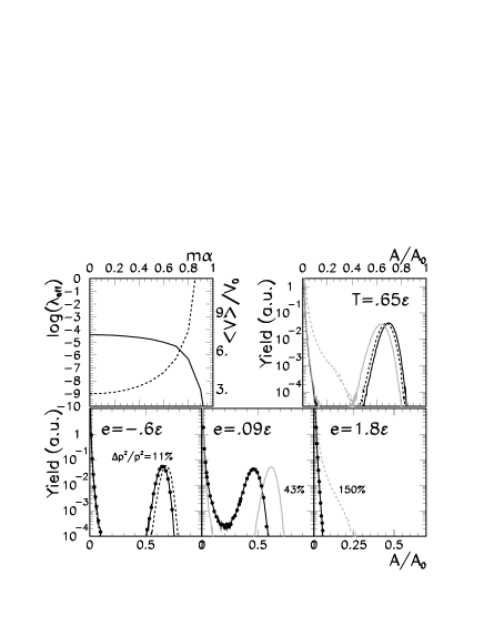
Figure 1: Upper left: effective pressure (full line) and average volume normalized to the ground state volume $V_{0}=A$ (dashed line) as a function of the collective radial flow. Upper right and lower part: fragment size distributions in the expanding Lattice Gas model. Distributions without flow (full black lines) are compared with distributions with 11% (dashed black), 43% (full grey) and 150% (dashed grey) contribution of radial flow at the same temperature (upper right) and at the same total energy (lower part).

As we have already mentioned in section IV, in the hypothesis of negligible interaction between the system’s constituents the expansion is self-similar, implying that the situation is equivalent to a standard Gibbs equilibrium in the local rest frame. In the expanding ensemble the total average kinetic energy per particle is simply the sum of the thermal energy $\langle e_{th}\rangle={3}/({2\beta})$ and the radial flow $\langle e_{fl}\rangle=m\alpha^{2}\langle r^{2}\rangle/2$.

This scenario is often invoked in the literature bondorf to justify the treatment of flow as a collective radial velocity superimposed on thermal motion; however eq.(11)contains also an additional term $\propto r^{2}$ which corresponds to an outgoing pressure . The phase diagram and fragment observables are therefore expected to be modified by the presence of flow even in the self similar approximation. To quantify this statement, we have performed calculations in the Lattice Gas Modelnpa , and the results are shown in Figure 1.

The effective pressure $\lambda_{eff}$ as well as the associated average volume are shown in the upper left part of figure 1 as a function of the collective radial flow for a given pressure and temperature . The Lagrange parameter $\lambda_{eff}$ being a decreasing function of $\alpha$, the critical point is moved towards higher pressures in the presence of flow jou . However one can see that the effect is very small up to $m\alpha\approx.6$ (which corresponds to $\Delta p^{2}/p^{2}=\langle e_{fl}\rangle/\langle e_{th}\rangle\approx 67\%$ flow contribution). In this regime the cluster size distributions displayed in the upper right part of figure 1 are only slightly affected. On the other side if collective flow overcomes a threshold value $\Delta p^{2}/p^{2}\approx 100\%$ the average volume shows an exponential increase and the outgoing flow pressure leads to a complete fragmentation of the system (dashed grey line in the lower part of fig.1). We can also observe that an oriented motion is systematically less effective than a random one to break up the system. This is shown in the lower part of figure 1 which compares for a given $\lambda$ distributions with and without radial flow at the same total deposited energy: for any value of radial flow equilibrium in the standard microcanonical ensemble corresponds to more fragmented configurations.

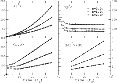
Figure 2: Time evolution of $<R^{2}>$, $<P^{2}>$ and $<R\cdot P>$ for an initially constrained Lennard Jones system of 147 particles freely expanding in the vacuum, at different total energies. Lower right: expansion dynamics (symbols) compared to the prediction of eq.(9) (lines).

The above results are relevant for the experimental situation if and only if the inter-fragment interactions can be neglected when the system is still compact enough to bear pertinent information on the phase diagram. Indeed only in this case the series (7) can be analytically summed up and the expansion dynamics can be reduced to a self similar flowannals . The validity of the ideal gas approximation eq.(9) for the expansion dynamics is tested in Figure 2matias in the framework of classical molecular dynamicsdorso . A Lennard Jones system is initially confined in a small volume and successively freely expanding in the vacuum. We can see that after a first phase of the order of $\approx 10$ Lennard Jones time units, where interparticle interactions cannot be neglected, the time evolution predicted by eq.(9) is remarkably fulfilled for all total energies. This result is due to the fact that the system’s size and dynamics are dominated by the free particles, while deviations from a self similar flow can be seen if the analysis is restricted to bound particlesmatias . We expect eq.(9) to describe the system evolution even better if the degrees of freedom $n$ are changed from particles to clusters, as suggested by the Fisher model of condensationfisher .

VI Conclusions

In this paper we have introduced an extension of Gibbs ensembles to time dependent constraints . This formalism gives a statistical description of a system observed at a time at which the entropy has not reached its saturating value yet, as it may be the case in intermediate energy heavy ion reactionslow:energy . Another physical application concerns systems for which the relevant observables pertain to different times, as in high energy nuclear collisions high:energy .

Our most important result is that any statistical description of a finite unbound system must necessarily contain a local collective velocity term. Indeed the knowledge of the average spatial extension of the system at a given time, naturally produces a flow constraint at any successive time. Conversely a collective flow measurement at a given time can be translated into an information on the system density at a former time.

References

- (1) E. T. Jaynes, ’Information theory and statistical mechanics’, Statistical Physics, Brandeis Lectures, vol.3, 160 (1963).
- (2) T. L. Hill, ’Thermodynamics of small systems’, W. A. Benjamin Inc., New York (1963).
- (3) F. Gulminelli, Ph. Chomaz, Phys. Rev. E 66 (2002) 46108
- (4) W. Thirring, H. Narnhofer, H. A. Posch, Phys. Rev. Lett. 91 (2003) 130601.
- (5) R. Balian, ’From microphysics to macrophysics’, Springer Verlag (1982).
- (6) Ph. Chomaz, F. Gulminelli, ’Phase transitions in finite systems, in Dynamics and thermodynamics of systems with long range interactions’, Lecture Notes in Physics vol.602, Springer (2002); F.Gulminelli, Ann.Phys.Fr., in press.
- (7) D. H. E. Gross, ’Microcanonical thermodynamics: phase transitions in finite systems’, Lecture Notes in Physics vol.66, Springer (2001).
- (8) J. P. Bondorf et al., Phys. Rep. 257 (1995) 133; F.Becattini et al., Phys.Rev. C69 (2004) 024905.
- (9) P. Braun-Munzinger et al., Invited review for Quark Gluon Plasma 3, eds. R. C. Hwa and Xin-Nian Wang, World Scientific Publishing.
- (10) The ensemble of events dynamically prepared may be characterized by an information about size and shape more complex than the simple mean square root radius. In this case other constraints can be introduced such as if the radii fluctuations contain non-trivial information or if the system is not spherical in average but has a finite quadrupole deformation.
- (11) Ph.Chomaz, F.Gulminelli and O.Juillet, Ann.Phys.,in press.
- (12) F. Gulminelli, Ph. Chomaz, Nucl. Phys. 734A (2004) 581.
- (13) J. Richert and P. Wagner, Phys. Rep. 350(2001) 1.
- (14) M.Ison et al., in preparation.
- (15) A. Chernomoretz et al., Nucl.Phys. A723 (2003) 229.
- (16) M. E. Fisher, Physics vol. 3, No.5 (1967) 255.
- (17) D.Jou et al., ’Thermodynamics of fluids under flow’, Springer (2001)