Correlation Functions: Getting into Shape

Abstract

The ability to measure characteristics of source shapes using non-identical particle correlations is discussed. Both strong-interaction induced and Coulomb induced correlations are shown to provide sensitivity to source shapes. By decomposing correlation functions with spherical or Cartesian harmonics, details of the shapes can be especially well isolated.

The space-time development of the expanding fireball in a heavy-ion collision at RHIC is driven by the pressure and viscosity of the matter during the novel stage of the reaction. Insight into these fundamental questions can be gained by understanding the spatio-temporal aspects of the collision. Correlation functions [1, 2, 3, 4] provide a direct link to the space-time structure of the source function, ${\cal S}({\bf P},{\bf r})$,

$$R({\bf P},{\bf q})=\int d^{3}r^{\prime}\left[\left|\phi({\bf q}^{\prime},{\bf r}^{\prime})\right|^{2}-1\right]S({\bf P},{\bf r}^{\prime}).$$ (1)

Here, $R({\bf P},{\bf q})+1$ is the ratio of two-particle cross-sections to the corresponding quantity for mixed-events, and is zero for uncorrelated emission. The source function $S({\bf P},{\bf r}^{\prime})$ measures the probability that two particles of the same velocity whose total momentum is ${\bf P}$ are separated by ${\bf r}$. The primes denote that the coordinates are measured in the rest frame of the pair. By measuring $R({\bf P},{\bf q})$ as a function of the relative momentum ${\bf q}^{\prime}=({\bf p}^{\prime}_{a}-{\bf p}^{\prime}_{b})/2$, one can exploit the structure of the relative wave function $\phi({\bf q}^{\prime},{\bf r}^{\prime})$ to extract information about $S({\bf P},{\bf r})$.

Understanding the source function in Eq. (1) assists in the determination of collective flow and lifetimes which directly address questions concerning the equation of state. In this talk the phenomenology that connects the source function to these important issues will be ignored. Instead, this talk focuses on the ability to determine size and shape information about $S({\bf r}^{\prime})$ from $R({\bf q}^{\prime})$. Thus, from this point on the total momentum label and the primes are suppressed. This problem can be considered as an inversion problem. Both $R({\bf q})$ and $S({\bf r})$ can be considered as vectors and $|\phi({\bf q},{\bf r})|^{2}$ can be considered as a matrix. Simply stated, Given $R({\bf q})$ and $|\phi({\bf q},{\bf r})|^{2}$, what can one determine about $S({\bf r})$? For non-interacting identical particles, $|\phi|^{2}=1+\cos 2{\bf q}\cdot{\bf r}$, and one can Fourier transform $R({\bf q})$ to find $S({\bf r})$. Our goal is to investigate the analogous deconvolution for wave functions whose forms are driven by Coulomb and strong interactions.

A straight-forward case to consider is interactions through classical Coulomb correlations. In the classical limit,

$$|\phi(q,r,\cos\theta_{qr})|^{2} \rightarrow \frac{d^{3}q_{0}}{d^{3}q}$$

$$= \frac{1+\cos\theta_{qr}-x}{\sqrt{(1+\cos\theta_{qr}-x)^{2}-x^{2}}}\Theta(1+\cos\theta_{qr}-2x),$$

where ${\bf q_{0}}$ is the relative momentum when the particles were separated by ${\bf r}$, $\theta_{qr}$ is the angle between ${\bf q}$ and ${\bf r}$, and $x=2\mu e^{2}/q^{2}r$. When integrating over angles, $|\phi|^{2}=\sqrt{1-x}$, and the correlation function approaches unity at large $q$ as $1-\langle 1/r\rangle\mu e^{2}/q^{2}$. By working inward from large $q$, the correlation function can be used to determine inverse moments of the source function, $1/r$, $1/r^{2}$, etc.

The $\cos\theta_{qr}$ dependence in Eq. (Correlation Functions: Getting into Shape) can be exploited to extract shape information about the source. This sensitivity is driven by the scattering of the Coulomb trajectories which lowers the population for angles where ${\bf q}$ leaves anti-parallel to ${\bf r}$ as illustrated in Fig. 1.

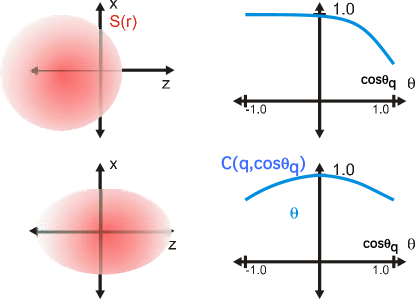
Fig. 1.: Coulomb repulsion suppresses trajectories where the outgoing relative momenta is anti-parallel to the original separation. For sources biased to one side, as illustrated in the upper panel, the correlation function is suppressed for opposite directions. For sources with a quadrapole distortion along a given axis, the distortion is strongest for emission parallel or anti-parallel to the axis as illustrated in the lower panel.

The quantum Coulomb wave function is more complex, and adds a additional sensitivity to $qr/\hbar$ in addition to $x$ and $\cos\theta_{qr}$. Quantum effects tend to smear out some of the sensitivity for $qr/\hbar\sim 1$ [5]. This especially harmful for small reduced masses, such as $\pi\pi$ correlations, since the correlations are smaller and need to be analyzed at smaller $q$. In fact, for cases where the Bohr radius is much larger than the source size ($a_{0}=1/\mu e^{2}=390$ fm for $\pi\pi$), the effect of Coulomb is a simple Gamow factor which is independent of $r$ and thus provides no information. Figure 2 shows correlations $pK^{+}$ correlations for a $4\times 4\times 8$ fm Gaussian source. Compared to classical correlations quantum correlations are somewhat muted, especially the shape information which is determined by looking at the dependence on the direction of ${\bf q}$. The muting is small for larger $q$, but there the correlation is small. Nonetheless, correlations are strong enough near 100 $MeV/c$ to determine shape characteristics of the source. The analogous calculations for Fig. 2 can be performed for any pair. Any interaction can be exploited to determine shape. For instance $p\Lambda$ interactions, which have no Coulomb, also provide sensitivity to shape through shadowing.

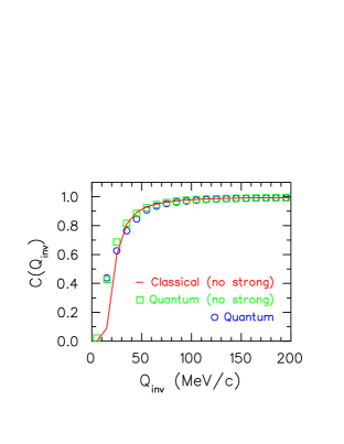
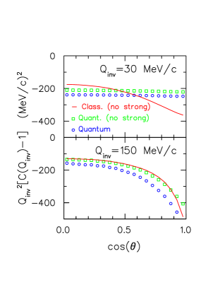
Fig. 2.: Proton-kaon correlation functions are shown for a $4\times 4\times 8$ fm Gaussian source. Quantum effects mute the sensitivity predicted from classical Coulomb trajectories. This especially true at low $Q=2q$. In the right-side panel, the correlation functions are scaled by $Q^{2}$ to counter the $1/Q^{2}$ fall-off. Incorporating strong interactions into the quantum calculations also affects the correlation.

In Figure 2 the anisotropy of the source was seen by plotting the correlation function as a function of $\cos\theta_{q}$, where $\theta_{q}$ was measured relative to the elongated axis. For more complicated three-dimensional shapes, especially where the source may not have reflection symmetries, determining characteristics of the shape can be more difficult. Spherical and Cartesian harmonics [6] can then be used to express the correlation function in terms of a few coefficients at small $\ell$. These expansion coefficients are themselves functions of $q$ and can be related to expansion coefficients for the source functions.

$$R_{\ell,m}(q)=\int 4\pi r^{2}dr~{}{\mathcal{K}}_{\ell}(q,r)~{}S_{\ell,m}(r),$$ (3)

where these quantities are related to the correlation function, wave function and source distribution by the following definitions,

$$R_{\ell,m}(q) \equiv (4\pi)^{-1/2}\int d\Omega_{q}R({\bf q})Y_{\ell,m}(\Omega_{q}),$$ (4)

$$S_{\ell,m}(r) \equiv (4\pi)^{-1/2}\int d\Omega_{r}S({\bf r})Y_{\ell,m}(\Omega_{r}),$$

$${\mathcal{K}}_{\ell}(q,r) \equiv \frac{1}{2}\int d\cos\theta_{qr}\left[|\phi(q,r,\cos\theta_{qr})|^{2}-1\right]P_{\ell}(\cos\theta_{qr}).$$

The convenience of this expression is that the expansion coefficients labeled $\ell$ and $m$ are related on a one-to-one basis with the corresponding coefficients in the source function.

The disadvantage with using spherical harmonics is that it can be difficult to physically visualize the distortion associated with a given $\ell$ and $m$, particularly for $\ell>2$. This can be remedied by using Cartesian harmonics. Cartesian harmonics of order $\ell=\ell_{x}+\ell_{y}+\ell_{z}$ are linear combinations of spherical harmonics of the same order. Each Cartesian harmonic is of the form,

$${\mathcal{A}}_{\vec{\ell}}(\hat{n})=n_{x}^{\ell_{x}}n_{y}^{\ell_{y}}n_{z}^{\ell_{z}}+{\rm~{}lower~{}orders~{}of~{}}n_{x},n_{y},n_{z}.$$ (5)

Some examples are given in Table 1. The disadvantage of Cartesian harmonics is that they are not orthonormal within a given $\ell$ multiplet. But, the $(2\ell+1)$ harmonics with $\ell_{x}=0,1$ can be used to easily generate the other functions with the identity, ${\mathcal{A}}_{\ell_{x},\ell_{y},\ell_{z}}=-{\mathcal{A}}_{\ell_{x}-2,\ell_{y}+2,\ell_{z}}-{\mathcal{A}}_{\ell_{x}-2,\ell_{y},\ell_{z}-2}$. Since Cartesian harmonics can be expressed as a linear combination of spherical harmonics of the same $\ell$,

$$R_{\vec{\ell}}(q)=\int 4\pi r^{2}dr~{}{\mathcal{K}}_{\ell}(q,r)~{}S_{\vec{\ell}}(r),$$ (6)

where the coefficients are defined,

$$R_{\vec{\ell}}(q) \equiv \frac{(2\ell+1)!!}{\ell!}\int\frac{d\Omega_{q}}{4\pi}R({\bf q}){\mathcal{A}}_{\vec{\ell}}(\Omega_{q}),$$ (7)

$$S_{\vec{\ell}}(q) \equiv \frac{(2\ell+1)!!}{\ell!}\int\frac{d\Omega_{q}}{4\pi}S({\bf q}){\mathcal{A}}_{\vec{\ell}}(\Omega_{q}).$$ (8)

References [6, 7] provide many properties of Cartesian harmonics and gives expressions for orthonormality, for transforming to spherical harmonics, and for generating moments.

Table 1.: Cartesian harmonics for $\ell<=4$. Other harmonics can be found by swapping indices on both sides of the equation, e.g., $x\leftrightarrow y$. For example, given ${\mathcal{A}}_{2,1,0}=n_{x}^{2}n_{y}-n_{y}/5$, swapping $y\leftrightarrow z$ gives ${\mathcal{A}}_{2,0,1}=n_{x}^{2}n_{z}-n_{z}/5$.

${\mathcal{A}}_{1,0,0}=n_{x}$	${\mathcal{A}}_{1,1,1}=n_{x}n_{y}n_{z}$
${\mathcal{A}}_{2,0,0}=n_{x}^{2}-(1/3)$	$A_{4,0,0}=n_{x}^{4}-(6/7)n_{x}^{2}+(3/35)$
${\mathcal{A}}_{1,1,0}=n_{x}n_{y}$	${\mathcal{A}}_{3,1,0}=n_{x}^{3}n_{y}-(3/7)n_{x}n_{y}$
$A_{3,0,0}=n_{x}^{3}-(3/5)n_{x}$	${\mathcal{A}}_{2,2,0}=n_{x}^{2}n_{y}^{2}-(1/7)n_{x}^{2}-(1/7)n_{y}^{2}+(1/35)$
${\mathcal{A}}_{2,1,0}=n_{x}^{2}n_{y}-(1/5)n_{y}$	${\mathcal{A}}_{2,1,1}=n_{x}^{2}n_{y}n_{z}-(1/7)n_{y}n_{z}$

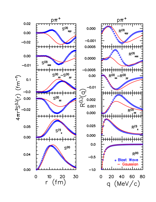
Fig. 3.: Decompositions in Cartesian harmonics of $p\pi^{+}$ source and correlation functions are shown for a blast-wave source (blue circles). A Gaussian source (Red), chosen to reproduce the integrated moments, does a poor job reproducing the source and correlation functions for some moments.

Results for various moments were generated for $p\pi$ correlations from a blast-wave model and are displayed in Fig. 3. The blast-wave temperature was chosen to be 120 MeV, the radius was 13 fm and the collective velocity was 0.7$c$. Since lighter particles tend to originate from deeper inside the blast wave, the source functions have strong dipole moments, which are manifest in the $\ell_{x}=1$ Cartesian projection, where $x$ refers to the outward direction. The $\ell=2$ moments describe the elliptic anisotropies, whereas the $\ell=1$ terms can be more directly identified with the offset of the center of the ellipse. The $(\ell_{x}=1,\ell_{y}=0,\ell_{z}=2)$ term is driven both by the combination of the offset and elliptic asymmetries and by the boomerang shape caused by the inside-outside geometry of the cascade. The non-Gaussian nature of the shape is seen by comparison with the best-fit Gaussian source. Gaussians are especially bad for fitting the behavior of the source function at larger $r$. Furthermore, the one-to-one correspondence for labels of the correlations and source function makes source imaging, which has been applied for angle-integrated correlations [8, 9, 10], tenable for higher harmonics.

One of the great benefits of analyses based on spherical or Cartesian harmonics is that the shape can be studied as a function of $r$. For instance, at RHIC the source functions should have exponential tails along the beam axis due to the boost-invariant nature of the expansion, and perhaps in the outward direction due to resonances. The higher harmonics should then be pronounced at large $r$ due to the decreasing justification of Gaussian fits. This is apparent in Fig. 3

Analyses such as those illustrated here can be performed for nearly every species measured at RHIC. For instance, with the last data run at RHIC, there should be enough data to analyze $\Sigma\pi$ correlations. There are dozens of possible analyses. In any model incorporating thermalization and collective flow, source sizes and shapes for different species should follow simple systematic trends driven by the particle masses. Observing such trends would be of tremendous importance in solidifying our understanding of collision dynamics at RHIC.

References

- [1] U.W. Heinz and B.V. Jacak, Ann. Rev. Nucl. Part. Sci. 49, 529 (1999).
- [2] C. Adler, et al., Phys. Rev. Lett. 87, 082301 (2002).
- [3] K. Adcox, et al., Phys. Rev. Lett. 88, 192302 (2002).
- [4] B.B. Back, et al., e-print, ArXiv.org:nucl-ex/0409001 (2004).
- [5] S. Pratt and S. Petriconi, Phys. Rev. C 68, 054901 (2003).
- [6] P. Danielewicz and S. Pratt, e-print, ArXiv.org:nucl-th/0501003 (2005).
- [7] J. Applequist, Theor. Chem. Acc. 107, 103 (2002).
- [8] D.A. Brown and P. Danielewicz, Phys. Rev. C 64, 014902 (2001).
- [9] S.Y. Panitkin et al., Phys. Rev. Lett. 87, 112304 (2001).
- [10] G. Verde et al., Phys. Rev. C 65, 054609 (2002).