Light front approach to correlations in hot quark matter

Abstract

We investigate two-quark correlations in hot and dense quark matter. To this end we use the light front field theory extended to finite temperature $T$ and chemical potential $\mu$. Therefore it is necessary to develop quantum statistics formulated on the light front plane. As a test case for light front quantization at finite $T$ and $\mu$ we consider the NJL model. The solution of the in-medium gap equation leads to a constituent quark mass which depends on $T$ and $\mu$. Two-quark systems are considered in the pionic and diquark channel. We compute the masses of the two-body system using a $T$-matrix approach.

1 Introduction

Light front (LF) quantization [1] provides a novel possibility to formulate quantum field theory at finite $T$ and $\mu$. Especially the phase diagram of quantum chromodynamics (QCD), that is tackled experimentally by relativistic heavy ion collisions and astrophysical observations may become accessible by LFQCD [2]. Here we introduce relativistic thermodynamics and quantum statistics in light front coordinates and as an application of light front techniques, we consider the pionic and scalar diquark channel of the Nambu Jona-Lasinio (NJL) model at finite temperature.

For the description of quark matter quantized on the light front plane one introduces coordinates $x^{\pm}=x^{0}\pm x^{3}$ and $x^{1,2}=x^{1,2}$ (see e.g. [2]). Contrary to the instant form in the front form all initial and boundary conditions of the fields are expressed on the plane $x^{+}=x^{0}+x^{3}=0$. The metric in the LF form has an off-diagonal form with $g^{++}=g^{--}=0$, $g^{+-}=2$ and $g^{ii}=-1$ for $i=1,2$. A major consequence of the front form is the on-shell relation, i.e. LF energy $k^{-}_{\rm on}$ is given by

$$k^{-}_{\rm on}=\frac{{\bf k}_{\perp}^{2}+m^{2}}{k^{+}}$$ (1)

with $k^{+}\not=0$. Note that there arises no sign ambiguity for the energy in contrast to the instant form.

The NJL Lagrangian for the two flavor case reads

$${\cal L}_{\rm NJL}=\bar{\psi}(i\gamma_{\mu}{\partial}^{\mu}-m_{0})\psi+G\left((\bar{\psi}\psi)^{2}+(\bar{\psi}i\gamma_{5}\mbox{\boldmath{$\tau$}}\psi)^{2}\right),$$ (2)

that is (approximately) invariant under chiral transformation due the small current quark mass $m_{0}$. Dynamical symmetry breaking leads to a gap equation for the quark mass. An extensive discussion on the NJL model and its implications for light mesons at finite temperature and density can be found in [3].

2 Quantum statistics on the light front

Our derivation of the statistical operator for a grand canonical ensemble is along Refs. [4, 5]. One starts with the von-Neumann equation for the LF time $x^{+}$, viz.

$$i\partial^{-}\hat{\varrho}=\left[\hat{P}^{-},\hat{\varrho}\right].$$ (3)

In thermodynamical equilibrium the left-hand side of (3) vanishes and the statistical operator $\hat{\varrho}$ depends only on the Poincaré generators that commute with the LF Hamiltonian $\hat{P}^{-}$. The explicit form of the operator $\hat{\varrho}$ follows from demanding the extremum of the entropy $S=-{\rm Tr}\left\{\hat{\varrho}\ln\hat{\varrho}\right\}$ under the constraints $T^{\mu\nu}={\rm Tr}(\hat{\varrho}\hat{T}^{\mu\nu})$ for the energy-momentum tensor and $j^{\mu}_{\ell}={\rm Tr}(\hat{\varrho}\hat{j}^{\mu}_{\ell})$ for all conserved currents of the system, i.e. the variation of entropy $\delta S$ under the constraint with respect to $\hat{\varrho}$ vanishes. Furthermore one identifies the Lagrange multipliers by comparing to the relativistic generalization of the Gibbs-Duhem relation [6]

$$\sigma^{\mu}=\theta_{\varrho}T^{\varrho\mu}+P\theta^{\mu}+\sum\limits_{A}\alpha_{A}j^{\mu}_{A},$$ (4)

where $\sigma^{\mu}$, P is the entropy flux and the invariant pressure. The four vector $\theta_{\mu}$ is given by $\theta_{\mu}=u_{\mu}/T$. Considering only the particle number $N$ as conserved quantity one has

$$\hat{\varrho}=\frac{1}{\cal Z}\exp\left\{-\frac{1}{T}\left(u_{\nu}\hat{P}^{\nu}-\mu\hat{N}\right)\right\},$$ (5)

where $u_{\nu}$ is the velocity of the medium.

Analogous to the instant form we compute the Fermi-Dirac distribution for an ideal gas of fermions. For the medium at rest, i.e. $u=(1,1,0,0)$ one obtains

$$f^{\pm}(k^{+},{\bf k}_{\perp})=\left[\exp\left\{\frac{1}{T}\left(\frac{1}{2}k^{-}_{\rm{on}}+\frac{1}{2}k^{+}\mp\mu\right)\right\}+1\right]^{-1},$$ (6)

where $f^{+}$($f^{-}$) is the distribution for quarks (antiquarks).

In the following we will need the in-medium quark propagator to take into account medium effects. Therefore one has to evaluate

$$i{\cal G}(x-y)=\theta(x^{+}-y^{+})\langle\psi(x)\bar{\psi}(y)\rangle-\theta(y^{+}-x^{+})\langle\bar{\psi}(y)\psi(x)\rangle.$$ (7)

The expectation value $\langle\dots\rangle$ indicates averaging over the grand canonical ensemble $\langle\dots\rangle={\rm Tr}(\hat{\varrho}\dots)$. A longer calculation (cf. [5]) leads to

$${\cal G}(k)= \frac{\gamma_{\mu}{k}_{\rm on}^{\mu}+m}{k^{+}}\left\{\theta(k^{+})\left(\frac{1-f^{+}(k^{+},{\bf k}_{\perp})}{k^{-}-k^{-}_{\rm on}+i\varepsilon}+\frac{f^{+}(k^{+},\bf{k}_{\perp})}{k^{-}-k^{-}_{\rm on}-i\varepsilon}\right)\right.$$ (8)

$$\left.+\theta(-k^{+})\left(\frac{f^{-}(-k^{+},{\bf k}_{\perp})}{k^{-}-k^{-}_{\rm on}+i\varepsilon}+\frac{1-f^{-}(-k^{+},{\bf k}_{\perp})}{k^{-}-k^{-}_{\rm on}-i\varepsilon}\right)\right\}.$$

The in-medium gap equation follows from $m=m_{0}-2G\langle\bar{\psi}\psi\rangle$ by a similar evaluation

$$m(T,\mu)=m_{0}+24G\int\limits_{\rm LB}\frac{dk^{+}d^{2}{\bf k}_{\perp}}{k^{+}(2\pi)^{3}}m(1-f^{+}(k^{+},{\bf k}_{\perp})-f^{-}(k^{+},{\bf k}_{\perp}))$$ (9)

which is regularized by an invariant Lepage-Brodsky (LB) cut-off [7].

3 Two-body systems

The two-body correlations are evaluated within a Bethe-Salpeter approach. We use a $T$-matrix equation with an appropriate interaction kernel induced by the Lagrangian (2). Bound states of mass $M$ show up as poles of the $T$-matrix $T(k)$ at $k^{2}=M^{2}$. First we consider the pionic channel and due to the zero-range interaction the $T$-matrix reduces to

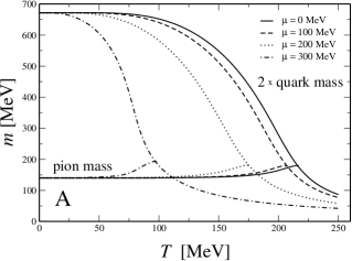
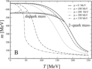
Fig. 1.: (A) The pion mass as a function of $T$ for different $\mu$. (B) The diquark mass as a function of $T$ for different $\mu$. The continuum is given by $2m$. The lines of the two-body masses end at the Mott dissociation points.

$$t_{\pi}(k)=\frac{-2iG}{1+2G\Pi_{\pi}(k^{2})}$$ (10)

with the pion loop integral $\Pi_{\pi}(k^{2})$ evaluated using (8)

$$\Pi_{\pi}(k^{2})=-6\int\limits_{\rm LB}\frac{dxd^{2}{\bf q}_{\perp}}{x(1-x)(2\pi)^{3}}\frac{M_{20}^{2}(x,{\bf q}_{\perp})\left(1-f^{+}(M_{20})-f^{-}(M_{20})\right)}{M_{20}^{2}(x,{\bf q}_{\perp})-k^{2}}.$$ (11)

Here $M_{20}^{2}(x,{\bf q}_{\perp})=({\bf q}_{\perp}^{2}+m^{2})/x(1-x)$ is the mass of the virtual two-body state. For the determination of the pion mass for given $T$ and $\mu$ one has to vary $k^{2}$ until the pole condition $1+2G\Pi_{\pi}(k^{2}=m_{\pi}^{2})=0$ holds. The results are presented in Fig. 1 (A).

A similar treatment like the pion case leads to the loop integral for a scalar, isospin singulet, color-antitriplet diquark [9]

$$\Pi_{s}(k^{2})=-6\int\limits_{\rm LB}\frac{dxd^{2}{\bf q}_{\perp}}{x(1-x)(2\pi)^{3}}\;\frac{M_{20}^{2}(x,{\bf q}_{\perp})\left(1-2f^{+}(M_{20})\right)}{M_{20}^{2}(x,{\bf q}_{\perp})-k^{2}}.$$ (12)

Here the pole condition takes the form $1+2G_{s}\Pi_{s}(k^{2}=m_{d}^{2})=0$, where $G_{s}$ is the coupling in the diquark channel which we treat as a parameter. The medium dependence of the diquark mass is shown in Fig. 1 (B).

4 Conclusions

We have shown that well-known properties of the NJL model are recovered in thermo field theory quantized on the light front. This includes the restoration of chiral symmetry and the dissociation of pion and diquark states. Since LF quantization is capable to treat the perturbative and nonpertubative part of QCD there is a perspective to explore the whole phase diagram of QCD at all values of temperature and chemical potential.

References

• [1] P.A.M.ย Dirac, Rev. Mod. Phys. 21, 392 (1949).
• [2] S.ย J.ย Brodsky, H.ย C.ย Pauli and S.ย S.ย Pinsky, Phys.ย Rept.ย  301 (1998) 299
• [3] S.ย P.ย Klevansky, Rev.ย Mod.ย Phys.ย  64 (1992) 649.
• [4] J.ย Raufeisen and S.ย J.ย Brodsky, Phys.ย Rev.ย D 70 (2004) 085017
• [5] M.ย Beyer, S.ย Mattiello, T.ย Frederico and H.ย J.ย Weber, J.ย Phys.ย G 31, 21 (2005).
• [6] W.ย Israel, Annals Phys.ย  100 (1976) 310; H.ย A.ย Weldon, Phys.ย Rev.ย D 26 (1982) 1394.
• [7] G.ย P.ย Lepage and S.ย J.ย Brodsky, Phys.ย Rev.ย D 22 (1980) 2157.
• [8] N.ย Ishii, W.ย Bentz and K.ย Yazaki, Nucl.ย Phys.ย A 587 (1995) 617; W.ย Bentz, T.ย Hama, T.ย Matsuki and K.ย Yazaki, Nucl.ย Phys.ย A 651 (1999) 143.
• [9] K.ย Rajagopal and F.ย Wilczek, arXiv:hep-ph/0011333.