A Realistic Calculation of the Effects of Nucleon-Nucleon Correlations in High-Energy Scattering Processes Off Nuclei

Abstract

A new linked cluster expansion for the calculation of ground state observables of complex nuclei with realistic interactions has been developed alv01 ; alv02 ; alv03 ; using the $V8^{\prime}$ pud01 potential the ground state energy, density and momentum distribution of complex nuclei have been calculated and found to be in good agreement with the results of fab01 , obtained within the Fermi Hyper Netted Chain, and Variational Monte Carlo pie01 approaches. Using the same cluster expansion, with wave function and correlations parameters fixed from the calculation of the ground-state observables, the semi-inclusive reaction of type $A(e,e^{\prime}p)X$ has been calculated taking final state interaction effects into account within a Glauber type calculation as in Ref. cio01 ; the comparison between the resulting distorted and undistorted momentum distributions provides an estimate of the transparency of the nuclear medium to the propagation of the hit proton. The effect of color transparency has also been considered within the approach of bra01 ; mor01 ; it is shown that at high values of $Q^{2}$ finite formation time effects strongly reduce the final state interaction, consistently with the idea of a reduced interaction of the hadron produced inside the nucleus bro01 . The total neutron-nucleus cross section at high energies has also been calculated alv04 by considering the effects of nucleon-nucleon correlations, which are found to increase the cross section by about 10% in disagreement with the experimental data. The inclusion of inelastic shadowing effects of Refs. gri01 ; jen01 decreases back the cross section, leading to a good agreement between experimental data and theoretical calculations.

I Introduction

The knowledge of the nuclear wave function, in particular its most interesting and poorly known part, viz the correlated one, is not only a prerequisite for understanding the details of bound hadronic systems, but is becoming at present a necessary ingredient for a correct description of medium and high energy scattering processes off nuclear targets; these in fact represent a current way of investigating short range effects in nuclei as well as those QCD effects (e.g. color transparency, hadronization, dense hadronic matter, etc) which manifest themselves in the nuclear medium. The necessity to treat nuclear effects in medium and high energy scattering within a realistic many body description, becomes therefore clear. The problem is not trivial, for one has first to solve the many body problem and then has to find a way to apply it to scattering processes. The difficulty mainly arises because even if a reliable and manageable many-body description of the ground state is developed, the problem remains of the calculation of the final state. In the case of few-body systems, a consistent treatment of Initial State Correlations (ISC) and final state interaction (FSI) is nowadays possible at low energies by solving the Schrödinger equation for the bound and continuum states but, at high energies, the Schrödinger approach becomes impractical and other methods have to be employed. In the case of complex nuclei, much remains to be done, also in view that the results of very sophisticated calculations ($e.g.$   the variational Monte Carlo ones pie01 ), show that the wave function which minimizes the expectation value of the Hamiltonian provides a very poor nuclear density; moreover, the structure of the best trial wave function is so complicated, that its use in the calculation of various processes at intermediate and high energies appears to be not easy task. It is for this reason that the evaluation of nuclear effects in medium and high energy scattering processes is usually carried out within simplified models of nuclear structure. As a matter of fact, initial state correlations ($ISC$) are often introduced by a procedure which has little to recommend itself, namely the expectation value of the transition operator is evaluated with shell model (SM) uncorrelated wave functions and the final state two-nucleon SM wave function is replaced by a phenomenological correlated wave function; to date, a consistent treatment of both ISC and FSI in intermediate and high energy scattering off complex nuclei is far from being completed, so that a quantitative and unambiguous evaluation of the role played ISC is still lacking. For such a reason we have undertaken the calculation of the ground-state properties (energies, densities and momentum distributions) of complex nuclei within a framework which can be easily generalized to the treatment of various scattering processes, keeping the basic features of ISC as predicted by the structure of realistic Nucleon-Nucleon (NN) interactions. This paper is organized as follows; in Section II the cluster expansion method is introduced, and the relevant ground state properties of ${}^{16}O$ and ${}^{40}Ca$ calculated. In Section III the semi-inclusive $A(e,e^{\prime}p)X$ reaction off complex nuclei targets is considered, and the FSI is calculated within the Glauber and Finite Formation Time pictures, taking advantage of the wave functions obtained in Section II. In Section IV the total neutron-nucleus cross section is calculated with the same wave functions, and the result of taking into account correlations and inelastic shadowing effects are discussed.

II The cluster expansion

We write the nuclear Hamiltonian in the usual form, i.e.:

$$\hat{H}\,=\,\hat{T}\,+\,\hat{V}\,=\,-\frac{\hbar^{2}}{2\,M_{N}}\,\sum^{A}_{i=1}\,\nabla^{2}_{i}\,\,+\,\sum_{i<j}\,\hat{v}_{2}(\mbox{\boldmath$x$}_{i},\mbox{\boldmath$x$}_{j})\;,$$ (1)

where the vector $x$ denotes the set of nucleonic degrees of freedom, and the two-body potential $\sum_{i<j}\,\hat{v}_{2}(\mbox{\boldmath$x$}_{i},\mbox{\boldmath$x$}_{j})$ is of the form

$$\hat{V}\,=\,\sum_{n=1}^{N}\,v^{(n)}(r_{ij})\,\hat{\mathcal{O}}^{(n)}_{ij}\,,$$ (2)

where $r_{ij}=|\mbox{\boldmath$r$}_{i}-\mbox{\boldmath$r$}_{j}|$ is the relative distance of nucleons $i$ and $j$, and $n$, ranging up to $N=18$, labels the state-dependent operator $\hat{\mathcal{O}}^{(n)}_{ij}$:

$$\hat{\mathcal{O}}^{(n)}_{ij}\,=\,\left[1\,,\,\mbox{\boldmath$\sigma$}_{i}\cdot\mbox{\boldmath$\sigma$}_{j}\,,\,\hat{S}_{ij}\,,\,\left(\mbox{\boldmath$S$}\cdot\mbox{\boldmath$L$}\right)_{ij}\,,\,L^{2},..\right]\,\otimes\,\left[1\,,\,\mbox{\boldmath$\tau$}_{i}\cdot\mbox{\boldmath$\tau$}_{j}\right]\,.$$ (3)

The evaluation of the expectation value of the nuclear Hamiltonian (1) is object of intensive activity which, in the last few years transp , has produced considerable results; nevertheless, the level of complexity of the obtained wave functions is such that they cannot be used in scattering problems with reasonable ease. Our goal is to present a more economical, but effective method for the calculation of the expectation value of any quantum mechanical operator $\hat{A}$

$$\langle\,\hat{A}\,\rangle\,=\,\frac{\langle\psi_{o}\,|\,\hat{A}\,|\,\psi_{o}\rangle}{\langle\psi_{o}\,|\psi_{o}\rangle}\,;$$ (4)

with $\psi_{o}$ having the following structure

$$\psi_{o}(\mbox{\boldmath$x$}_{1},...,\mbox{\boldmath$x$}_{A})\,=\,\hat{F}(\mbox{\boldmath$x$}_{1},...,\mbox{\boldmath$x$}_{A})\,\phi_{o}(\mbox{\boldmath$x$}_{1},...,\mbox{\boldmath$x$}_{A})\,,$$ (5)

where $\phi_{o}$ is a Shell-Model (SM), mean-field wave function, and $\hat{F}$ is a symmetrized correlation operator, which generates correlations into the mean field wave function. According to the two-body interaction of Eq. (2), the correlation operator is cast in the following form:

$$\hat{F}(\mbox{\boldmath$x$}_{1},\mbox{\boldmath$x$}_{2}\,...\,\mbox{\boldmath$x$}_{A})\,=\,\hat{S}\,\prod^{A}_{i<j}\,\hat{f}(r_{ij})$$ (6)

with

$$\hat{f}(r_{ij})=\sum_{n=1}^{N}\,\hat{f}^{(n)}(r_{ij})\;\;\hskip 56.9055pt\hat{f}^{(n)}(r_{ij})=f^{(n)}(r_{ij})\,\hat{O}^{(n)}_{ij}\,.$$ (7)

In the present paper we are going to introduce a cluster expansion technique in order to evaluate Eq. (4); the solution can be found by applying the variational principle, with the variational parameters contained both in the correlation functions and in the mean field single particle wave functions. The expectation value $\langle\hat{A}\rangle$ defined in (4) can be expanded in the framework of the cluster expansion developed in Refs. alv01 ; alv02 ; alv03 and, at first order, it reads as follows

$$\langle\hat{A}\rangle_{1}=\langle\phi_{o}\,|\sum_{i<j}\left(\hat{f}_{ij}\hat{A}\hat{f}_{ij}-\hat{A}\right)|\,\phi_{o}\rangle-\langle\hat{A}\rangle_{o}\langle\phi_{o}\,|\sum_{i<j}\left(\hat{f}_{ij}\hat{f}_{ij}-1\right)|\,\phi_{o}\rangle\,,$$ (8)

where $\langle\hat{A}\rangle_{o}$ is given by $\langle\phi_{o}\,|\hat{A}|\,\phi_{o}\rangle$ The $2nd$ order term can straightforwardly be obtained by the same technique used to derive Eq. (8) Given the two-body interaction as in Eq. (2), the expectation value of the Hamiltonian can be written in the following way:

$$E_{o} = -\,\frac{\hbar^{2}}{2\,M_{N}}\,\int d\mbox{\boldmath$r$}_{1}\left[\nabla_{1}\,\cdot\,\nabla_{1^{\prime}}\,\,\rho^{(1)}(\mbox{\boldmath$r$}_{1},\mbox{\boldmath$r$}_{1}^{\prime})\right]_{\mbox{\boldmath$r$}_{1}=\mbox{\boldmath$r$}_{1}^{\prime}}\,+$$ (9)

$$\hskip 56.9055pt+\,\sum_{n}\;\int\;d\mbox{\boldmath$r$}_{1}d\mbox{\boldmath$r$}_{2}\;v^{(n)}(r_{12})\rho^{(2)}_{(n)}(\mbox{\boldmath$r$}_{1},\mbox{\boldmath$r$}_{2})\,,$$

where $\rho^{(1)}(\mbox{\boldmath$r$}_{1},\mbox{\boldmath$r$}_{1}^{\prime})$ and $\rho^{(2)}_{(n)}(\mbox{\boldmath$r$}_{1},\mbox{\boldmath$r$}_{2})$ are the non-diagonal One Body Density Matrix (OBDM) and the (spin and isospin dependent-; see Ref. alv01 ) Two Body Density (TBD) matrices, respectively These can be calculated from the ground state wave function by inserting in Eq. (4) the corresponding operators. The knowledge of the OBDM and TBD matrices allows one to calculate, besides the ground-state energy, other relevant quantities like e.g. the density distribution:

$$\rho(\mbox{\boldmath$r$})\,=\,\rho^{(1)}(\mbox{\boldmath$r$}_{1}=\mbox{\boldmath$r$}_{1}^{\prime}\equiv\mbox{\boldmath$r$})\,,$$ (10)

and the nucleon momentum distribution, defined as:

$$n(\mbox{\boldmath$k$})\,=\,\frac{1}{(2\pi)^{3}}\,\int d\mbox{\boldmath$r$}_{1}d\mbox{\boldmath$r$}^{\prime}_{1}\,e^{i\,\mbox{\boldmath$k$}\cdot(\mbox{\boldmath$r$}_{1}-\mbox{\boldmath$r$}^{\prime}_{1})}\,\rho(\mbox{\boldmath$r$}_{1},\mbox{\boldmath$r$}^{\prime}_{1})\,.$$ (11)

The results of calculation of the ground state energy, the charge density and the two-body density and momentum distribution using the realistic $V8^{\prime}$ interaction pud01 is discussed in detail in Ref. alv01 ; alv02 ; alv03 .

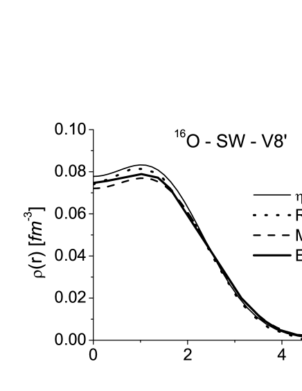
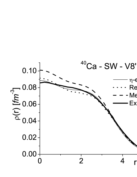
Figure 1: The charge densities of ${}^{16}O$ (left) and ${}^{40}Ca$ (right) calculated within the cluster expansion compared with the experimental data. The mean field result and the results of the FHNC calculation of Ref. fab01 are also shown.

In Fig. 3 we show the effect of correlations on the charge density and the two-body density of ${}^{16}O$. In the case of charge density, we have shown the three contributions which arises from the first-order cluster expansion, i.e., the mean field, hole and spectator contributions, which are shown in Fig. 4 in a diagrammatic picture. In the case of two-body density, we compare the mean field result with the ones obtained taking into account the only central correlation ($f_{1}$ approximation) and the first six correlations ($N=6$ in Eq. (7); $f_{6}$ approximation).

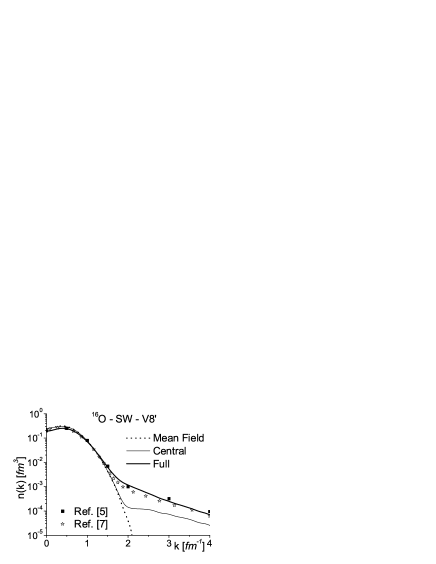
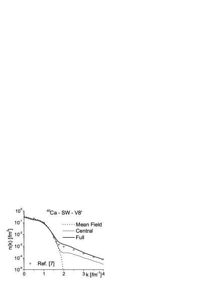
Figure 2: The momentum distributions of ${}^{16}O$ (left) and ${}^{40}Ca$ (right) calculated within the cluster expansion, compared with the mean field result and with the FHNC approach of Ref. fab01 and the VMC approach of Ref. pie01 .

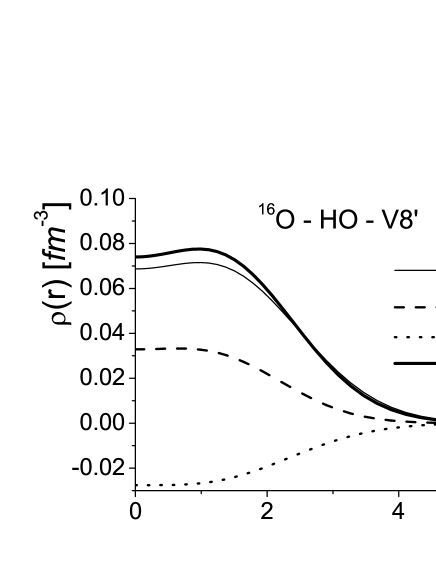
Figure 3: Effect of correlations versus the non-correlated result for the charge density (left) and the two-body density (right) of ${}^{16}O$ calculated within the cluster expansion.

a)

b)

c)

Figure 4: Diagrammatic representation of the one body mixed density matrix $\rho(\mbox{\boldmath$r$}_{1},\mbox{\boldmath$r$}^{\prime}_{1})$ in the lowest order of the $\eta$-expansion (Eq. (10)). a) is the shell model contribution and b) and c) the $hole$ and spectator contributions, respectively. The direct and exchange contributions are shown on the left and right sides of the Figure, respectively.

III Applications. I - the semi-inlcusive process $A(e,e^{\prime}p)X$

Using the cluster expansion developed in in the Section II, we have calculated the semi-inclusive $A(e,e^{\prime}p)X$ process in which an electron with 4-momentum $k_{1}\equiv\{{\bf k}_{1},i\epsilon_{1}\}$, is scattered off a nucleus with 4-momentum $P_{A}\equiv\{{\bf 0},iM_{A}\}$ to a state $k_{2}\equiv\{{\bf k}_{2},i\epsilon_{2}\}$ and is detected in coincidence with a proton $p$ with 4-momentum $p\equiv\{{\bf p},iE_{p}\}$; the final $(A-1)$ nuclear system with 4-momentum $P_{X}\equiv\{{\bf P}_{X},iE_{X}\}$ is undetected. The cross section for the exclusive process $A(e,e^{\prime}p)B$ can be written as follows

$$\frac{d\sigma}{dQ^{2}d\nu d{\bf p}}=K\sigma_{ep}P_{D}(E_{m},{\bf p}_{m})$$ (12)

where $K$ is a kinematical factor, $\sigma_{ep}$ the off-shell electron-nucleon cross section, and $Q^{2}=|{\bf q}|^{2}-\nu^{2}$ the four momentum transfer. The quantity $P_{D}(E_{m},{\bf p}_{m})$ is the distorted nucleon spectral function which depends upon the observable missing momentum ${\bf p}_{m}={\bf q}-{\bf p}$ (${\bf p}_{m}=-{\bf k}$ when the FSI is absent) and missing energy $E_{m}=\nu-T_{p}-T_{A-1}$. In the semi-inclusive $A(e,e^{\prime}p)X$ process, the cross section (12) is integrated over the missing energy $E_{m}$, at fixed value of ${\bf p}_{m}$ and becomes directly proportional to the distorted momentum distribution

$$n_{D}({\bf p}_{m})={(2\pi)^{-3}}\int e^{i{\bf p}_{m}\,\cdot\,({\bf r}_{1}-{\bf r}_{1}^{\prime})}\rho_{D}({\bf r}_{1},{\bf r}_{1}^{\prime})\,d{\bf r}_{1}d{\bf r}_{1}^{\prime}$$ (13)

where

$$\rho_{D}({\bf r}_{1},{\bf r}_{1}^{\prime})=\frac{\langle\psi_{o}\,S^{\dagger}\,\hat{\rho}({\bf r}_{1},{\bf r}_{1}^{\prime})\,S^{\prime}\,{\psi_{o}}^{\prime}\rangle}{\langle\psi_{o}\,\psi_{o}\rangle}$$ (14)

is the distorted one-body mixed density matrix, $S$ is the S-matrix describing FSI and

$$\hat{\rho}_{1}(\mbox{\boldmath$\tilde{r}$}_{1},\mbox{\boldmath$\tilde{r}$}_{1}^{\prime})\,=\,\sum_{i}\,\delta(\mbox{\boldmath$r$}_{i}-\mbox{\boldmath$\tilde{r}$}_{1})\,\delta(\mbox{\boldmath$r$}_{i}^{\prime}-\mbox{\boldmath$\tilde{r}$}^{\prime}_{1})\,\prod_{j\neq i}\,\delta(\mbox{\boldmath$r$}_{j}-\mbox{\boldmath$r$}^{\prime}_{j})$$ (15)

is the one-body density matrix operator; the primed quantities have to be evaluated at ${\bf r}_{i}^{\prime}$ with $i=1,...,A$. The integral of $n_{D}({\bf p}_{m})$ gives the integrated nuclear transparency $T$

$$T=\frac{\int n_{D}({\bf p}_{m})\,d{\bf p}_{m}}{\int n(k)\,d{\bf k}}=\int\rho_{D}({\bf r})\,d{\bf r}=1+\Delta T$$ (16)

where $\rho_{D}({\bf r})=\rho_{D}({\bf r}_{1}={\bf r}^{\prime}_{1}\equiv{\bf r})$ and $\Delta T$ originates from the FSI. In Ref. cio01 Eq. (13) has been evaluated using a Glauber representation for the scattering matrix $S$, viz

$$S\rightarrow S_{G}({\bf r}_{1}\dots{\bf r}_{A})=\prod_{j=2}^{A}G({\bf r}_{1},{\bf r}_{j})\equiv\prod_{j=2}^{A}\bigl{[}1-\theta(z_{j}-z_{1})\Gamma({\bf b}_{1}-{\bf b}_{j})\bigr{]}$$ (17)

where ${\bf b}_{j}$ and $z_{j}$ are the transverse and the longitudinal components of the nucleon coordinate ${\bf r}_{j}\equiv({\bf b}_{j},z_{j})$, ${\mit\Gamma}({\bf b})$ the Glauber profile function for elastic proton nucleon scattering, and the function $\theta(z_{j}-z_{1})$ takes care of the fact that the struck proton “1” propagates along a straight-path trajectory so that it interacts with nucleon “$j$” only if $z_{j}>z_{1}$. Generalizing the same cluster expansion described in Section II to take into account Glauber rescattering, we have obtained the distorted nucleon momentum distributions $n_{D}({\bf p}_{m})=n_{D}(p_{m},\theta)$, where $\theta$ is the angle between ${\bf q}$ and ${\bf p}_{m}$; the results for ${}^{16}O$ and ${}^{40}Ca$ are presented in Fig. 5.

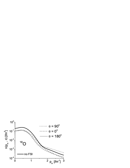
Figure 5: The distorted momentum distribution, $n_{D}({\bf p}_{m})=n_{D}(p_{m},\theta)$ ($\theta=\widehat{{\bf q}{\bf p}}_{m}$), of ${}^{16}O$ and ${}^{40}Ca$, obtained by Eq. (13).

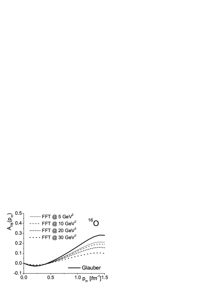
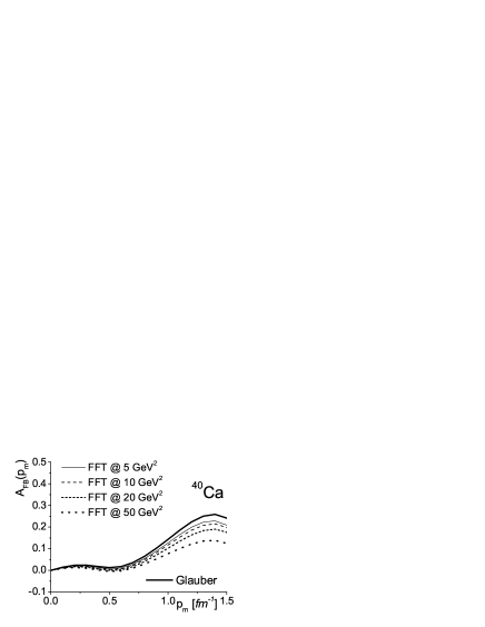
Figure 6: The forward-backward asymmetry (Eq. 20) for the process $A(e,e^{\prime}p)X$, with $A=16$ and $A=40$, calculated within the Glauber approach (solid thick line) taking into account the Finite Formation Time (FFT) mechanism of various values of the 4-momentum transfer.

The Glauber multiple scattering picture can be implemented by taking into account Finite Formation Time (FFT) introduced in Ref. bra01 , where it has been shown that at the values of the Bjorken scaling variable $x=Q^{2}/2m\nu\simeq 1$, FFT effects can be treated in a simple way, i.e. by replacing the Glauber operator (Eq. (17)) with

$$S_{FFT}({\bf r}_{1},...,{\bf r}_{A})=\,\,\prod^{A}_{j=2}\Big{(}1-J(z_{1}-z_{j})\Gamma({\bf b}_{1}-{\bf b}_{j})\Big{)}\,,$$ (18)

where

$$J(z)\,=\,\theta(z)\,\Big{(}1\,-\,e^{-\,z\,\frac{x\,m\,M^{2}}{Q^{2}}}\Big{)}\,$$ (19)

$m$ being the nucleon mass and $M^{2}=m^{*\,2}-m^{2}$ is a parameter describing the average excitation energy of the ejectile. It can be seen that at sufficiently high values of $Q^{2}$, $J\rightarrow 0$ and the FSI vanishes; this new mechanism for the description of FSI is inspired by the QCD prediction of color transparency, which states that a pointlike, color-less particle, such as the object singled out by the virtual photon interaction with the nuclear medium at high $Q^{2}$, should have reduced cross-section with the nuclear medium as long as it does not evolve into a physical proton inside the nucleus. We have calculated the effect of FFT on the forward-backward asymmetry, defined in Ref. bia01 as

$$A_{FB}\,=\,\frac{n_{D}(p_{m},\theta=0^{o})\,-\,n_{D}(p_{m},\theta=180^{o})}{n_{D}(p_{m},\theta=0^{o})\,+\,n_{D}(p_{m},\theta=180^{o})}$$ (20)

and the results are shown in Fig. 6.

IV Applications. II - the total neutron-nucleus cross section

The neutron-Nucleus ($n-A$) total cross section, $\sigma^{tot}_{nA}$ is defined by the optical theorem as

$$\sigma_{tot}=\frac{4\pi}{k}Im\left[F_{00}(0)\right]\,;$$ (21)

where, within the Glauber eikonal approximation, the elastic scattering amplitude has the following form:

$$F_{00}(\mbox{\boldmath$q$})=\frac{ik}{2\pi}\int e^{i{\bf q}\cdot{\bf b_{n}}}\langle\psi_{o}|\{1-\hat{S}_{G}\}|\psi_{o}\rangle=\frac{ik}{2\pi}\int d^{2}b_{n}e^{i{\bf q}\cdot{\bf b_{n}}}\left[1-\mathbf{e^{i\,\chi_{opt}({\bf b}_{n})}}\right]$$ (22)

with

$$\mathbf{e^{i\,\chi_{opt}(\mbox{\boldmath$b$}_{n})}}\,=\,\int\prod_{j=1}^{A}d\mbox{\boldmath$r$}_{j}\,G(\mbox{\boldmath$b$}_{n},\mbox{\boldmath$s$}_{j})\,\left|\psi_{o}(\mbox{\boldmath$r$}_{1},...,\mbox{\boldmath$r$}_{A})\right|^{2}\delta\left(\frac{1}{A}\sum{\bf r}_{j}\right)\,,$$ (23)

where $\mbox{\boldmath$r$}_{j}\equiv(\mbox{\boldmath$s$}_{j},z_{j})$ and $\mbox{\boldmath$b$}_{n}$ is the neutron impact parameter. As it is well known the squared wave function can be written in terms of density distributions as follows alv04 :

$$\left|\,\psi_{o}\,(\mbox{\boldmath$r$}_{1},...,\mbox{\boldmath$r$}_{A})\,\right|^{2}\,=\,\prod_{j=1}^{A}\,\rho(\mbox{\boldmath$r$}_{j})\,+\,\sum_{i<j}^{A}\,\mathbf{\Delta(\mbox{\boldmath$r$}_{i},\mbox{\boldmath$r$}_{j})}\,\prod_{k\neq(ij)}^{A}\,\rho(\mbox{\boldmath$r$}_{k})\,+\,...$$ (24)

where $\rho(\mbox{\boldmath$r$})$ is the one-body density distribution and the two-body contraction $\Delta$ is defined in terms of one- and two- body density distributions, $\rho^{(2)}(\mbox{\boldmath$r$}_{1},\mbox{\boldmath$r$}_{2})$:

$$\mathbf{\Delta(\mbox{\boldmath$r$}_{1},\mbox{\boldmath$r$}_{2})}\,=\,\left[\rho^{(2)}(\mbox{\boldmath$r$}_{1},\mbox{\boldmath$r$}_{2})\,-\,\rho^{(1)}(\mbox{\boldmath$r$}_{1})\,\rho^{(1)}(\mbox{\boldmath$r$}_{2})\right]\,;$$ (25)

Usually Glauber-type calculations are based upon the single density approximation, consisting in disregarding all terms of Eq. (24) but the first one. We have considered, for the first time, also the second term of the expansion (24) i.e. the effects of two-body correlations. In the case of ${}^{4}He$ we have also considered three- and for-body correlations alv04 ; whereas for ${}^{4}He$ Eq. (24) has been used, for heavier nuclei we have used its optical limit ($A>>1$) in Eq. (23) i.e.

$$\mathbf{e^{i\,\chi_{opt}(\mbox{\boldmath$b$}_{n})}} \simeq exp\left[-\,A\,\int d\mbox{\boldmath$r$}_{1}\,\rho(\mbox{\boldmath$r$}_{1})\,\Gamma(\mbox{\boldmath$b$}_{n}-\mbox{\boldmath$s$}_{1})\right.\,+$$ (26)

$$+\,\left.A^{2}\,\frac{\int d\mbox{\boldmath$r$}_{1}d\mbox{\boldmath$r$}_{2}\,\mathbf{\Delta(\mbox{\boldmath$r$}_{1},\mbox{\boldmath$r$}_{2})}\,\Gamma(\mbox{\boldmath$b$}_{n}-\mbox{\boldmath$s$}_{1})\,\Gamma(\mbox{\boldmath$b$}_{n}-\mbox{\boldmath$s$}_{2})}{1-\int d\mbox{\boldmath$r$}_{1}\,\rho(\mbox{\boldmath$r$}_{1})\,\Gamma(\mbox{\boldmath$b$}_{n}-\mbox{\boldmath$s$}_{1})}\right]\,;$$

which already for $A\geq 12$ reproduces the results based upon Eq. (24) almost exactly. We have evaluated the one- and two-body density matrices appearing in Eq. (26) starting from the realistic wave functions obtained in Section II.

The results of calculations are shown in Fig. 8. It can be seen that the inclusion of correlations in the target wave function produce an enhancement of the cross section of about $10\%$ with respect to the mean field result, increasing the disagreement with the experimental data.

     

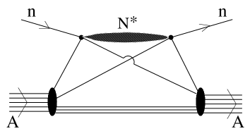
a)                                               b)

Figure 7: The neutron-nucleus total cross section diagrams. a) Glauber double scattering; b) inelastic shadowing effects.

It is well known however that at high energies diffractive scattering of the projectile, depicted if Fig. 7, plays a relevant role. We have evaluated such an effect (also known as Gribov inelastic shadowing) according to Refs. gri01 ; jen01 . It can be seen that inelastic shadowing effects play indeed a relevant role to bring theoretical calculations in good agreement with experimental data.

     

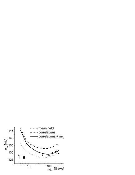
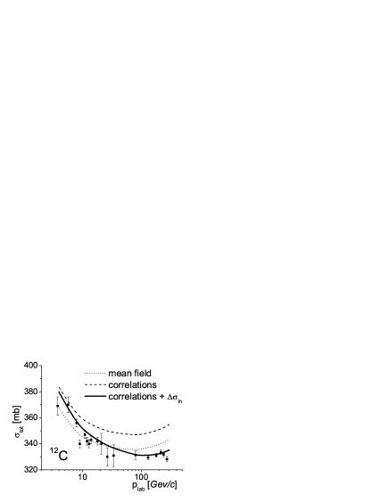
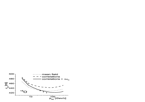
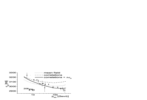
Figure 8: The double scattering diagrams in the neutron-nucleus total cross section.

V Summary

We have developed a method which can be used to calculate scattering processes at medium and high energies within a realistic and parameter-free description of nuclear structure. Our calculations followed the following strategy: i) the values of the parameters pertaining to the correlation functions and the mean field wave functions, have been obtained from the calculation of the ground-state energy, radius and density of the nucleus, to a given order of the expansion, using realistic nucleon-nucleon interactions; ii) using these parameters we have calculated, by a proper generalization of the cluster expansion, the distorted momentum distributions, the nuclear transparency and the total neutron-nucleus cross section. The method we have developed appears to be a very effective, transparent and parameter-free one. To sum up, we have shown that, using realistic models of the nucleon-nucleon interaction, a proper approach based on cluster expansion techniques can produce reliable approximations for those diagonal and non diagonal density matrices which appear in various medium and high energy scattering processes off nuclei, so that the role of nuclear effects in these processes can be reliably estimated without using free parameters to be fitted to the data.

VI Acknowledgments

We are grateful to the organizers for the invitation to the Workshop. HM would like to thank the Department of Physics, University of Perugia and INFN, Sezione di Perugia, for warm hospitality and support. Support by the Italian Ministero dell’Istruzione, Università e Ricerca (MIUR), through the contracts COFIN03-029498 and COFIN04-025729, is gratefully acknowledged.

References

- (1) M. Alvioli, C. Ciofi degli Atti, H. Morita, Phys. Rev. C (2005); in press.
- (2) M. Alvioli, PhD Thesis, University of Perugia (2003).
- (3) M. Alvioli, C. Ciofi degli Atti, H. Morita, Fizica B13 585 (2004).
- (4) B. S. Pudliner, V. R. Pandharipande, J. Carlson, S. C. Pieper and R. B. Wiringa, Phys. Rev. C56 (1999) 1720.
- (5) A. Fabrocini, F. Arias de Saavedra and G. Co’, Phys. Rev. C61, 044302 (2000) and Private Communication.
- (6) S.C. Pieper, R.B. Wiringa and V.R. Pandharipande, Phys. Rev. C46, 1741 (1992).
- (7) C. Ciofi degli Atti, and D. Treleani, Phys. Rev C60 (1999) 024602.
- (8) M. A. Braun, C. Ciofi degli Atti and D. Treleani, Phys. Rev. C62 (2001) 034606.
- (9) H. Morita, M. A. Braun, C. Ciofi degli Atti and D. Treleani, Nucl. Phys. A699 (2002) 328c.
- (10) S. J. Brodsky and A. H. Mueller, Phys. Lett. B206 (1988) 685
- (11) M. Alvioli, C. Ciofi degli Atti, I. Marchino and H. Morita, in preparation
- (12) V. N. Gribov, Sov JETP 29 (1969) 483; J. Pumplin, M. Ross, Phys. Rev. Lett. 21 (1968) 1778; V. A. Karmanov,L. A. Kondratyuk, Jetp letters 18 (1973) 451.
- (13) B. K. Jennings and G. A. Miller, Phys. Rev. C49 (1999) 2637.
- (14) A. Mueller, in Prooceedings of the 17th rencontre de Moriond, edited by J. Tranh Thanh Van (Edition Frontieres, Gif-sur-Ivette, 1982), p. 13; S. J. Brodsky, in Prooceedings of the 13th International Symposium on Multiparticle Dynamics, edited by E. W. Kittel, W. Metzger, and A. Stergiou (World Scientific, Singapore, 1982), p. 964.
- (15) L. L. Foldy and J. D. Walecka, Ann. Phys. 54 (1969) 447.
- (16) A. Bianconi, S. Jeshonnek, N.N. Nikolaev and B.G. Zakharov, Phys. Lett. B343 (1995) 13.