Effects of mode-mode and isospin-isospin correlations on domain formation of disoriented chiral condensates

Abstract

The effects of mode-mode and isospin-isospin correlations on nonequilibrium chiral dynamics are investigated by using the method of the time dependent variational approach with squeezed states as trial states. Our numerical simulations show that large domains of the disoriented chiral condensate (DCC) are formed due to the combined effect of the mode-mode and isospin-isospin correlations. Moreover, it is found that, when the mode-mode correlation is included, the DCC domain formation is accompanied by the amplification of the quantum fluctuation, which implies the squeezing of the state. However, neither the DCC domain formation nor the amplification of the quantum fluctuation is observed if only the isospin-isospin correlation is included. This suggests that the mode-mode coupling plays a key role in the DCC domain formation.

I Introduction

The possibility of the formation of the disoriented chiral condensate (DCC) in relativistic heavy ion collisions has been investigated in a number of theoretical studies. Non-equilibrium field dynamics has been studied also in conjunction with the structure formation in early universe. Within the classical approximation it has been recognized that large domains of DCC are produced during the nonequilibrium process in the course of the time evolution from the quench initial condition ref:classical01 ; ref:classical02 . On the other hand, in calculations including quantum mechanical effects, mainly homogeneous (translationally invariant) systems have been studied to avoid technical difficulty in numerically calculating the two-point functions boyanovski01 ; cooper01 . In fact, there have been several attempts to include spatial inhomogeneity cooper02 ; smit ; bettencourt and also memory effect berges ; ikeda in the quantum mechanical time evolution of the fields. However, the correlation between modes with different momenta (mode-mode correlation) was not taken into account in these works and the effect of interactions has been included only through the mean fields. It has not been settled whether large domain structure is formed when quantum effects are taken into account.

Recently, it was explicitly shown that DCC domains are formed in quantum calculation for the first time in the case of 1+1 dimensional geometry IAT . In that calculation, the mode-mode correlations are explicitly taken into account and no translational invariance was assumed. The importance of the mode-mode correlation is qualitatively understood as follows. If one does not include the mode-mode correlation, each mode is decoupled from each other during the time evolution except for the indirect interactions through the mean fields. The energy transfer from modes with short wavelengths to those with long wavelengths is not effective enough to form large correlated domains. If one includes the mode-mode correlation, direct energy transfer from short wavelength modes to long wavelength modes and as a result the amplification of long wavelength modes in the pion fields become possible, which can lead to the formation of large DCC domains.

In this paper, in addition to the mode-mode correlation, we examine the effect of the correlation between fields having different isospin components (isospin-isospin correlation). This effect on the domain formation of the DCC has not been given particular attention to in earlier studies. However, the isospin-isospin correlation can arise during the nonequilibrium process as well as the mode-mode correlation. It is important to incorporate both correlations on an equal footing. In addition, it is of interest to study whether the isospin-isospin correlation affects the domain formation of DCC and, if yes, it is then important to compare the ways the two correlations affect the domain formation. We also make further examination on the quantum mechanical features of the domain formation in this paper.

The rest of the paper is organized as follows. In Section II we briefly review the formalism and the equations of motion, and discuss the initial condition. In Section III, we present numerical results. Section IV is devoted to summary and conclusions.

II Equations of Motion and Initial Condition

We take the O(4) linear sigma model as a low energy effective theory of QCD and apply the method of the time dependent variational approach (TDVA) with squeezed states as trial states as in the previous paper IAT . This method was originally developed by Jackiw and Kerman as an approximation in the functional Schrödinger approach JK and later it was shown to be equivalent to TDVA with squeezed states by Tsue and Fujiwara TF . This method makes it possible to solve the time-evolution of the order parameters (mean fields), and the quantum fluctuations and correlations in a self-consistent manner.

II.1 Equations of motion

We denote the sigma ($\sigma({\vec{x}})$) and pion $({\vec{\pi}}({\vec{x}})$) field operators as a four dimensional vector, $\phi_{a}({\vec{x}})=(\sigma({\vec{x}}),{\vec{\pi}}({\vec{x}}))$, where $a$ runs from 0 to 3. Then the Hamiltonian $H$ of the O(4) linear sigma model is given as

$$H = \int\sum_{a=0}^{3}\biggl{\{}\frac{1}{2}{\pi}_{a}({\vec{x}})^{2}+\frac{1}{2}{\vec{\nabla}}{\phi}_{a}({\vec{x}})\cdot{\vec{\nabla}}{\phi}_{a}({\vec{x}})+\lambda\bigl{[}{\phi}({\vec{x}})^{2}-v^{2}\bigr{]}^{2}-h{\phi}_{0}({\vec{x}})\biggr{\}}d{\vec{x}}$$ (1)

$$= \int\sum_{a=0}^{3}\biggl{\{}\frac{1}{2}{\pi}_{a}({\vec{x}})^{2}+\frac{1}{2}{\vec{\nabla}}{\phi}_{a}({\vec{x}})\cdot{\vec{\nabla}}{\phi}_{a}({\vec{x}})+V[\phi({\vec{x}})]\biggr{\}}d{\vec{x}},$$

where ${\phi}({\vec{x}})^{2}=\sum_{a=0}^{3}{\phi}_{a}({\vec{x}})^{2}$, and $\lambda$, $v$, and $h$ are constants. Note that ${\pi}_{a}({\vec{x}})$ is the conjugate field operator of $\phi_{a}({\vec{x}})$ and should not be confused with the pion field operator. We determine the three model parameters, $\lambda$, $v$, and $h$, so that they give the pion mass $M_{\pi}=138$ MeV, the sigma meson mass $M_{\sigma}=500$ MeV, and the pion decay constant $f_{\pi}=93$ MeV in the one loop level in the “broken symmetry” vacuum state as in the previous study, i.e., $\lambda=3.44$, $v=110$ MeV, and $h=(103~{}{\rm MeV})^{3}$ IAT ; TKI .

The squeezed states used as trial states have the following form:

$$|\Phi(t)\rangle = \exp\left\{i\sum_{a=0}^{3}\int\left(D_{a}({\vec{x}},t)\phi_{a}({\vec{x}})-C_{a}({\vec{x}},t)\pi_{a}({\vec{x}})\right)d{\vec{x}}\right\}$$ (2)

$$\times \mathcal{N}(t)\exp\Biggl{\{}\sum_{a,b=0}^{3}\int\phi_{a}({\vec{x}})\Bigl{(}\frac{1}{4}G_{ab}^{(0)-1}({\vec{x}},{\vec{x}^{\prime}})-\frac{1}{4}G_{ab}^{-1}({\vec{x}},{\vec{x}^{\prime}},t)+i\Pi_{ab}({\vec{x}},{\vec{x}^{\prime}},t)\Bigr{)}\phi_{b}({\vec{x}})d{\vec{x}}d{\vec{x}^{\prime}}\Biggr{\}}|0\rangle.$$

Here $|0\rangle$ is the vacuum state, and $G_{aa}^{(0)}({\vec{x}},{\vec{y}})=\langle 0|\phi_{a}({\vec{x}})\phi_{a}({\vec{y}})|0\rangle$ and $G_{ab}^{(0)}({\vec{x}},{\vec{y}})=0$ for $a\neq b$. $C_{a}({\vec{x}},t)$ and $D_{a}({\vec{x}},t)$ are the c-number mean fields of $\phi_{a}({\vec{x}})$ and $\pi_{a}({\vec{x}})$, respectively. $G_{ab}({\vec{x}},{\vec{y}},t)$ and $\Pi_{ab}({\vec{x}},{\vec{y}},t)$ are the quantum correlation functions having isospin indices $a$ and $b$ (quantum fluctuation if both ${\vec{x}}={\vec{y}}$ and $a=b$ hold), and the canonical conjugate variable for $G_{ab}({\vec{x}},{\vec{y}},t)$, respectively. Thus, the trial state is specified by $C_{a}({\vec{x}},t)$, $D_{a}({\vec{x}},t)$, $G_{ab}({\vec{x}},{\vec{y}},t)$, and $\Pi_{ab}({\vec{x}},{\vec{y}},t)$. All of these variables are real. $\mathcal{N}(t)$ is a normalization constant, whose explicit form is not needed in the calculation of the time evolution of observables. Its explicit expression is given in Ref. TF . When there is no isospin-isospin correlation, the above squeezed state reduces to the direct product of the squeezed states with single isospin labels, $a=0\sim 3$. The squeezed state include the coherent state as a special case. In addition, correlations can also be taken into account with the trial states. Thus, the trial states given by Eq. (2) span a wide subspace in the physical Hilbert space and are expected to be able to describe a variety of quantum features of the system.

The time evolution is determined by the time dependent variational principle:

$$\delta\int\langle\Phi(t)|i\frac{\partial~{}}{\partial t}-H|\Phi(t)\rangle dt=0.$$ (3)

The equations of motion in momentum space read

$$\ddot{C}_{a}({\vec{k}},t) = -{\vec{k}}^{2}C_{a}({\vec{k}},t)-\mathcal{M}_{a}^{(1)}({\vec{k}},t),$$

$$\dot{G}_{ab}({\vec{k}},{\vec{k}^{\prime}},t) = 2\sum_{a^{\prime}=0}^{3}\langle{\vec{k}}|\Bigl{[}G_{aa^{\prime}}(t)\Pi_{a^{\prime}b}(t)+\Pi_{aa^{\prime}}(t)G_{a^{\prime}b}(t)\Bigr{]}|{\vec{k}^{\prime}}\rangle,$$

$$\dot{\Pi}_{ab}({\vec{k}},{\vec{k}^{\prime}},t) = \frac{1}{8}\sum_{a^{\prime}=0}^{3}\langle{\vec{k}}|G_{aa^{\prime}}^{-1}(t)G_{a^{\prime}b}^{-1}(t)|{\vec{k}^{\prime}}\rangle-2\sum_{a^{\prime}=0}^{3}\langle{\vec{k}}|\Pi_{aa^{\prime}}(t)\Pi_{a^{\prime}b}(t)|{\vec{k}^{\prime}}\rangle-\frac{1}{2}(2\pi)^{3}{\vec{k}}^{2}\delta_{ab}\delta^{3}({\vec{k}}-{\vec{k}^{\prime}})-\frac{1}{2}\mathcal{M}_{ab}^{(2)}({\vec{k}}-{\vec{k}^{\prime}},t),$$

$$\mathcal{M}_{a}^{(1)}({\vec{k}},t) = \Bigl{[}-m^{2}C_{a}({\vec{k}},t)+\int\frac{d{\vec{l}}d{\vec{l}^{\prime}}}{(2\pi)^{6}}\Big{(}4\lambda C_{a}({\vec{k}}-{\vec{l}}-{\vec{l}^{\prime}},t)\sum_{b=0}^{3}C_{b}({\vec{l}},t)C_{b}({\vec{l}^{\prime}},t)+12\lambda C_{a}({\vec{k}}-{\vec{l}}-{\vec{l}^{\prime}},t)G_{aa}({\vec{l}},{\vec{l}^{\prime}},t)$$

$$+4\lambda C_{a}({\vec{k}}-{\vec{l}}-{\vec{l}^{\prime}},t)\sum_{b(\neq a)}G_{bb}({\vec{l}},{\vec{l}^{\prime}},t)+8\lambda\sum_{b(\neq a)}C_{b}({\vec{k}}-{\vec{l}}-{\vec{l}^{\prime}},t)G_{ba}({\vec{l}},{\vec{l}^{\prime}},t)\Bigr{)}-h\delta_{a0}V\Bigr{]},$$

$$\mathcal{M}_{aa}^{(2)}({\vec{k}},t) = -m^{2}V+\int\frac{d{\vec{l}}}{(2\pi)^{3}}\Bigl{(}12\lambda\bigl{(}C_{a}({\vec{k}}-{\vec{l}},t)C_{a}({\vec{l}},t)+G_{aa}({\vec{k}}-{\vec{l}},{\vec{l}},t)\bigr{)}$$

$$+4\lambda\sum_{b(\neq a)}\bigl{(}C_{b}({\vec{k}}-{\vec{l}},t)C_{b}({\vec{l}},t)+G_{bb}({\vec{k}}-{\vec{l}},{\vec{l}},t)\bigr{)}\Bigr{)},$$

$$\mathcal{M}_{ab(\neq a)}^{(2)}({\vec{k}},t) = 8\lambda\int\frac{d{\vec{l}}}{(2\pi)^{3}}\Bigl{(}C_{a}({\vec{k}}-{\vec{l}},t)C_{b}({\vec{l}},t)+G_{ab}({\vec{k}}-{\vec{l}},{\vec{l}},t)\Bigr{)},$$ (4)

where $m^{2}=4\lambda v^{2}$ and $V={\rm Tr}{\bf 1}=\int d{\vec{x}}$. $C_{a}({\vec{k}},t)$ is the mean field for the $\phi_{a}$ field with momentum ${\vec{k}}$, and $G_{ab}({\vec{k}},{\vec{k}^{\prime}},t)$ and $\Pi_{ab}({\vec{k}},{\vec{k}^{\prime}},t)$ are the correlation between modes with isospins $a$ and $b$, and momenta ${\vec{k}}$ and ${\vec{k}^{\prime}}$ (the quantum fluctuation for $a=b$ and ${\vec{k}}={\vec{k}^{\prime}}$), and the canonical conjugate variable for $G_{ab}({\vec{k}},{\vec{k}^{\prime}},t)$, respectively. The one-point functions $C_{a}({\vec{k}},t)$ and $D_{a}({\vec{k}},t)$ and the two-point functions $G_{ab}({\vec{k}},{\vec{k}^{\prime}},t)$ and $\Pi_{ab}({\vec{k}},{\vec{k}^{\prime}},t)$ are the momentum space representations of $C_{a}({\vec{x}},t)$, $D_{a}({\vec{x}},t)$, $G_{ab}({\vec{x}},{\vec{x}^{\prime}},t)$, and $\Pi_{ab}({\vec{x}},{\vec{x}^{\prime}},t)$, respectively. In Eq. (4), we have used the following notation,

$$\langle{\vec{k}}|H(t)I(t)|{\vec{k}^{\prime}}\rangle=\frac{1}{(2\pi)^{3}}\int H({\vec{k}},{\vec{k}^{\prime\prime}},t)I({\vec{k}^{\prime\prime}},{\vec{k}^{\prime}},t){d{\vec{k}^{\prime\prime}}}.$$ (5)

$\mathcal{M}_{ab}^{(2)}({\vec{k}},t)$ in Eq. (4) originates from the nonlinear coupling term in the Hamiltonian and is given as follows:

$$\mathcal{M}_{ab}^{(2)}({\vec{k}},t) = \int\mathcal{M}_{ab}^{(2)}({\vec{x}},t)e^{i{\vec{k}}\cdot{\vec{x}}}{d{\vec{x}}},$$

$$\mathcal{M}_{ab}^{(2)}({\vec{x}},t) = \exp\left\{\frac{1}{2}\sum_{a^{\prime},b^{\prime}=0}^{3}\frac{\partial}{\partial z_{a^{\prime}}}G_{a^{\prime}b^{\prime}}({\vec{x}},{\vec{x}},t)\frac{\partial}{\partial z_{b^{\prime}}}\right\}$$ (6)

$$\left.\times\frac{\partial^{2}}{\partial z_{a}\partial z_{b}}U[z]\right|_{z_{a}=C_{a}({\vec{x}},t)},$$

where $U[z]$ represents the c-number potential that is obtained by replacing $\phi_{a}$ in the potential term of the model Hamiltonian $V[\phi]$ by $z_{a}\in{\bf R}$:

$$U[z]=\left.\phantom{\frac{}{}}V[\phi]\right|_{\phi_{a}({\vec{x}})\,=\,z_{a}}\quad(a\,=\,0-3).$$ (7)

The third equation in Eq. (4) tells us that mode-mode correlations in momentum space arise through $\mathcal{M}_{ab}^{(2)}({\vec{k}}-{\vec{k}^{\prime}},t)$ with $\vec{k}\neq\vec{k}^{\prime}$ even if there is initially no such correlation. Similarly, the isospin-isospin correlation arise due to the interaction term $\mathcal{M}^{(2)}_{ab}({\vec{k}}-{\vec{k}^{\prime}},t)$ with $a\neq b$.

In the numerical calculation, we assume that the system is in a cubic box with the volume $V=L^{3}$ and complies the periodic boundary condition, and that the lattice spacing in each direction is the same, $d=\frac{L}{N}$, where $N$ is the division number in each direction. Accordingly, the momentum $\vec{k}$, the square momentum $\vec{k}^{2}$, and the momentum integral in Eq. (4) are replaced as follows:

$${\vec{k}} \rightarrow \frac{2\pi}{L}{\vec{n}},$$

$${\vec{k}}^{2} \rightarrow \sum_{i=x,y,z}\frac{4}{d^{2}}\sin^{2}\left(\frac{\pi n_{i}}{N}\right),$$

$$\int\frac{d{\vec{k}}}{(2\pi)^{3}} \rightarrow \frac{1}{V}\sum_{n_{x}=0}^{N-1}\sum_{n_{y}=0}^{N-1}\sum_{n_{z}=0}^{N-1},$$ (8)

with $\vec{n}=(n_{x},n_{y},n_{z})$.

II.2 Initial condition

As the initial condition, we take the quench initial condition. In the quench scenario, the following assumption on the time evolution of the system is made: The matter produced in relativistic heavy-ion collisions is initially thermalized and that chiral symmetry is restored. Then, this matter goes through rapid cool down and the true vacuum spontaneously breaks chiral symmetry. In this process, however, the change of the effective potential is so rapid that the order parameter cannot follow the change and remains around the origin, where the minimum of the effective potential is in the chirally symmetric phase. ref:classical01 ; ref:classical02 ; IAT . Namely, in the quench scenario, the mean of the chiral fields as well as the correlation of the fields are the same as those before the sudden cooling (quenching), but only the sizes of the fluctuations of the mean fields and their conjugate fields are quenched. In order to realize the quench scenario in our numerical calculation, we specify the initial condition for the mean fields and the quantum correlation and fluctuation as follows.

For the mean fields, we have used the same prescription for the initial condition as in Refs. IAT ; AM : at each grid site, the mean field variables for the chiral fields and their conjugate variables $C_{a}({\vec{x}},0)$ and $D_{a}({\vec{x}},0)$ are randomly distributed with the Gaussian weights with the following parameters,

$$\langle C_{a}({\vec{x}},0)\rangle = 0,$$

$$\langle C_{a}({\vec{x}},0)^{2}\rangle-\langle C_{a}({\vec{x}},0)\rangle^{2} = \delta^{2},$$

$$\langle D_{a}({\vec{x}},0)\rangle = 0,$$

$$\langle D_{a}({\vec{x}},0)^{2}\rangle-\langle D_{a}({\vec{x}},0)\rangle^{2} = \frac{D}{d^{2}}\delta^{2},$$ (9)

where $\delta$ is the Gaussian width and $D$ is the spatial dimension. In relating the Gaussian widths of $C_{a}({\vec{x}},0)$ and $D_{a}({\vec{x}},0)$, we have taken advantage of the virial theorem. For detailed discussion on the use of virial theorem, see Ref. AM . We use the Gaussian width $\delta=0.19v$, which is the same value which has been taken in Ref. IAT . This value is so chosen that the fluctuation is small enough and the chiral symmetry is spontaneously broken. This is necessary to ensure that the quench scenario is simulated. This value of $\delta$ is taken as a typical value and, of course, other choices are also possible.

In order to fix the initial condition for the quantum correlation and fluctuation, we have assumed that each of the sigma and pion states in momentum space is independently in a coherent state with a degenerate mass $m_{0}$. Accordingly, $G_{ab}({\vec{x}},{\vec{y}},0)$ and $\Pi_{ab}({\vec{x}},{\vec{y}},0)$ are given as follows:

$$G_{aa}({\vec{x}},{\vec{y}},0) = \frac{1}{(2\pi)^{3}}\int_{0}^{\Lambda}\frac{e^{i{\vec{k}}\cdot({\vec{x}}-{\vec{y}})}}{2\omega_{k}}d{\vec{k}},$$

$$G_{ab(\neq a)}({\vec{x}},{\vec{y}},0) = 0,$$

$$\Pi_{ab}({\vec{x}},{\vec{y}},0) = 0,$$ (10)

with $\omega_{k}=\sqrt{m_{0}^{2}+{\vec{k}}^{2}}$. We adopt $m_{0}=200$ MeV. The two-point functions $G_{ab}({\vec{x}},{\vec{y}},0)$ and $\Pi_{ab}({\vec{x}},{\vec{y}},0)$ are thus diagonal in both momentum and isospin spaces in the initial state. However, as previously explained, their off-diagonal components in both momentum and isospin spaces arise through the non-linear coupling term in the equation of motion Eq. (4), if the mean field is not translationally invariant in coordinate space or symmetric in isospin space. We examine the effect of these off-diagonal components of the Green’s function on the time evolution of the system in the next section.

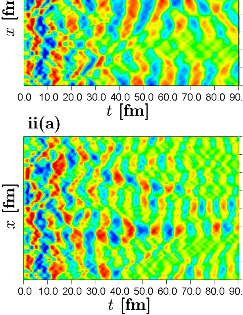
Figure 1: (Color online) Time evolution of the mean field of the third component of the pion field in cases i(a), i(b), ii(a), and ii(b).

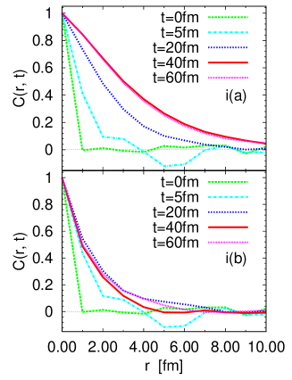
Figure 2: (Color online) Snap shots of the spatial correlations of the mean fields in case i(a) and case i(b).

Figure 3: (Color online) Snap shots of the spatial correlations of the mean fields in case ii(a) and case ii(b).

III Numerical Results

We evolve the mean fields and the two-point functions on a discrete lattice with the total length in the $z$ direction $L=64$ fm and the lattice spacing $d=1.0$ fm, which corresponds to the three dimensional momentum cutoff $\Lambda=1071$ MeV. We assume translational invariance in the $x$ and $y$ directions, thus $D=1$ in Eq. (9). We have confirmed that the total energy is conserved at least to an accuracy of less than 1 percent throughout the time evolution.

To understand the role of the mode-mode and isospin-isospin correlations separately, we have performed the following four numerical simulations:
Case i(a): The mode-mode and the isospin-isospin correlations are both included.
Case i(b): The mode-mode correlation is ignored, but the isospin-isospin correlation is included.
Case ii(a): The mode-mode correlation is included, but the isospin-isospin correlation is ignored.
Case ii(b): The mode-mode and the isospin-isospin correlations are both ignored.

III.1 Time evolution of the mean fields

First we show the time evolution of the mean fields. Figure 1 illustrates the time evolution of the mean field of the third component of the pion field in the four cases. The value of the mean field is represented by different colors at each position and time.

In case i(a) and case ii(a), where the mode-mode correlation is included, the formation of the domain structure of the pion field is clearly seen. Also it is observed that the size of the domains continues to grow beyond the time scale of the rolling down, $\sim$a few fm, in these cases. On the contrary, the formation of only small domains is observed in case i(b) and case ii(b). In these cases, the mode-mode correlation is not included and short range fluctuation is dominant throughout the time evolution. No qualitative change in the behavior of the mean fields is observed after a few fm. These results imply that the mode-mode correlation is a key ingredient for the DCC domain formation.

Furthermore, it is observed that the domain structure is larger in case i(a), where the mode-mode and isospin-isospin correlations are both included, compared with case ii(a), where only the mode-mode correlation is included. The appearance of the larger domains in case i(a) is due to the combined effect of mode-mode and isospin-isospin correlations. Also it is observed that in case i(b), where the isospin-isospin correlation is included but the mode-mode correlation is not included, domains are slightly larger compared to those in case ii(b), where either correlation is not included. From these results, we find that the domain formation is most effective when both mode-mode and isospin-isospin correlations are included.

III.2 Spatial Correlation

In this subsection, we show the spatial correlation function $C(r,t)$ defined by

$$C(r,t)=\frac{\int{{\vec{C}}}({\vec{x}})\!\cdot\!{{\vec{C}}}({\vec{y}})\delta(|{\vec{x}}-{\vec{y}}|-r)d{\vec{x}}d{\vec{y}}}{\int|{{\vec{C}}}({\vec{x}})||{{\vec{C}}}({\vec{y}})|\delta(|{\vec{x}}-{\vec{y}}|-r)d{\vec{x}}d{\vec{y}}}~{},$$ (11)

where ${{\vec{C}}}({\vec{x}})\!\cdot\!{{\vec{C}}}({\vec{y}})=\sum_{i=1}^{3}{C_{i}}({\vec{x}}){C_{i}}({\vec{y}})$ and $|{{\vec{C}}}({\vec{x}})|=\sqrt{\sum_{i=1}^{3}{C_{i}}({\vec{x}})^{2}}$. This is a measure for the closeness of the order parameters in isospin space at distance $r$ in coordinate space.

The snap shots of the spatial correlations at $t=0$ (the initial time), 5, 20, 40, and 60 fm are shown in Figs. 3 and 3 for the four cases. The correlation functions are obtained by taking the ensemble average over 10 independent initial states. At the initial time $t=0$, the spatial correlation length is almost equal to the lattice spacing in each case. This is so, because the initial mean fields are independently distributed at each grid site. However, difference in the correlation function appears as the time elapses.

The correlation lengths in the upper figures are always longer than those in the lower figures in both Fig. 3 and Fig. 3. This tells us the importance of the mode-mode correlation in the trial quantum states in the growth of the correlation length regardless of the presence of the isospin-isospin correlation. Moreover, the correlation length in case i(a) is longer than in case ii(a), while that in case i(b) is only a little longer than in case ii(b). The formation of larger DCC domains is induced by the combined effect of the mode-mode correlation and the isospin-isospin correlation.

The duration of the correlation generation differs between cases i(a) and i(b), and between cases ii(a) and ii(b). However, it is almost the same in cases i(a) and ii(a), and in cases i(b) and ii(b). In cases i(b) and ii(b), the formation of the correlation almost finishes by $t=5$ fm, which is the typical time scale within which the rolling-down of the order parameter from the top of the effective potential is completed gm . We will explicitly show this in the next subsection. The fact that the correlation increases beyond that time scale in cases i(a) and ii(a) strongly suggests that the mode-mode coupling is another driving force for the domain formation in addition to the instability of the low momentum modes that exists during the rolling-down of the order parameter ref:classical01 .

As a possible mechanism of DCC formation, the parametric resonance has been also proposed ref:parametric . It is, however, also understood within the framework of the mean field theory without correlations among modes; it is in essence a one-mode problem. Thus, the mode-mode coupling is yet another mechanism for DCC formation, and according to the result of our calculation, it has the most dominant effect on the generation of the field correlations. It is interesting to compare this result with the result of the classical simulation by Rajagopal and Wilczek ref:classical01 . In their work, it was found that the amplification of low momentum modes lasts far beyond the typical time scale of the rolling-down of the order parameter. Their calculation is classical, but includes direct couplings among modes. This also exemplifies the importance of the direct mode-mode coupling in the domain formation.

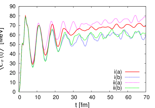
Figure 4: (Color online) Time evolution of the spatial average of the sigma field in cases i(a), i(b), ii(a), and ii(b).

III.3 Time evolution of the sigma field

In this subsection, we examine whether there is the collective oscillation of the sigma field, which is required for the DCC domain formation through the parametric resonance. For this purpose, we show the time evolution of the spatial average of the sigma field defined by,

$$\langle C_{0}(t)\rangle=\frac{1}{V}\int C_{0}({\vec{x}},t)d{\vec{x}}.$$ (12)

Note that the zeroth component of the chiral field is the sigma field.

Figure 4 shows the time evolution of the spatial average of the sigma field in the four cases. This result was obtained by taking the ensemble average over 10 initial states. In each case the sigma field quickly rolls down from the top of the effective potential and approaches its ground state value within less than 5 fm. After that, the sigma field continues to oscillate as found in earlier studies ref:classical01 ; ref:classical02 . The oscillation is damped more quickly in cases i(a) and ii(a), where the direct mode-mode coupling is taken into account. In case i(a), the oscillation almost disappears by $t=25$ fm. On the other hand, according to Fig. 3, the correlation length of the pion field continues to grow until about $t=40$ fm. Thus, the collective oscillation of the sigma field is not necessarily needed for the DCC domain formation unlike in the parametric resonance scenario.

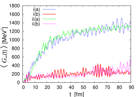
Figure 5: (Color online) Time evolution of the spatial average of the quantum fluctuation of the third component of the pion field, $\langle G_{33}(t)\rangle$ in cases i(a), i(b), ii(a), and ii(b).

III.4 Quantum fluctuations

In this subsection, we show the time evolution of the quantum fluctuation.

Figure 5 depicts the time evolution of the spatial average of the quantum fluctuation of the third component of the pion field, $\langle G_{33}(t)\rangle$, which is defined by,

$$\langle G_{33}(t)\rangle=\frac{1}{V}\int G_{33}({\vec{x}},{\vec{x}},t)d{{\vec{x}}}.$$ (13)

In this figure, no event average is taken. However, since the spatial size of the system is large enough, the behavior of $\langle G_{11}(t)\rangle$ and $\langle G_{22}(t)\rangle$ is expected to be similar to that of $\langle G_{33}(t)\rangle$ due to the isospin symmetry.

In the initial state, fluctuation is small. This is because the initial state is chosen to be the direct product of the coherent states. The remarkable feature is that the quantum fluctuation is substantially amplified in the cases with the mode-mode correlation, i.e., cases i(a) and ii(a). On the other hand, such substantial amplification of the quantum fluctuation is absent in the cases without mode-mode correlation, i.e., cases i(b) and ii(b). In addition, it is noted that the duration of the amplification of the quantum fluctuation in cases i(a) and i(b) is of the same order as that of the correlation formation observed in Fig. 3. In the space of the trial states, the amplification of the quantum fluctuation implies squeezing of the states. Thus, the main part of the late time DCC domain formation occurs in concurrence with squeezing of the states.

On the contrary, only little difference in the time evolution of the quantum fluctuation is observed between cases i(a) and i(b), and also between cases ii(a) and ii(b). This implies that the isospin-isospin correlation does not lead to further amplification of the quantum fluctuation.

However, we have observed that there is a little difference in the formation of correlations between cases i(a) and i(b), and also between cases ii(a) and ii(b), in Figs. 3 and 3. This suggests that there are at least two mechanisms that lead to the long range correlation of the pion fields: one that is accompanied by the squeezing of the pion fields and the other that is not.

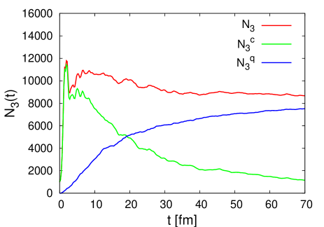
Figure 6: (Color online) Time evolution of the total particle numbers of the third component of the pion field $N_{3}$, its classical part $N_{3}^{cl}$, and its quantum part $N_{3}^{q}$ in case ii(a).

III.5 Pion particle numbers

In this subsection, we calculate the particle numbers associated with the pion fields for cases ii(a) and ii(b).

In order to analyze the particle numbers associated with the pion fields, we expand the field operator $\phi_{a}({\vec{x}})$ and its conjugate operator $\pi_{a}({\vec{x}})$ by the annihilation operator ${\hat{a}}_{a}({\vec{k}})$ and creation operator ${\hat{a}}_{a}^{\dagger}({\vec{k}})$ of the pion with the momentum ${\vec{k}}$ and isospin $a$,

$$\phi_{a}({\vec{x}}) = \frac{1}{(2\pi)^{3}}\int\sqrt{\frac{1}{2\omega_{k}}}\left[{\hat{a}}_{a}({\vec{k}})e^{i{\vec{k}}\cdot{\vec{x}}}+{\hat{a}}_{a}^{\dagger}({\vec{k}})e^{-i{\vec{k}}\cdot{\vec{x}}}\right]{d{\vec{k}}},$$

$$\pi_{a}({\vec{x}}) = \frac{1}{i(2\pi)^{3}}\int\sqrt{\frac{\omega_{k}}{2}}\left[{\hat{a}}_{a}({\vec{k}})e^{i{\vec{k}}\cdot{\vec{x}}}-{\hat{a}}_{a}^{\dagger}({\vec{k}})e^{-i{\vec{k}}\cdot{\vec{x}}}\right]{d{\vec{k}}},$$

where $\omega_{k}$ is the energy of the normal modes with the pion mass in the vacuum $M_{\pi}$, $\omega_{k}=\sqrt{M_{\pi}^{2}+{\vec{k}}^{2}}$. From these relations, we obtain

$${\hat{a}}_{a}({\vec{k}}) = \int\left[\sqrt{\frac{\omega_{k}}{2}}\phi_{a}({\vec{x}})+i\sqrt{\frac{1}{2\omega_{k}}}\pi_{a}({\vec{x}})\right]e^{-i{\vec{k}}\cdot{\vec{x}}}d{\vec{x}},$$

$${\hat{a}}_{a}^{\dagger}({\vec{k}}) = \int\left[\sqrt{\frac{\omega_{k}}{2}}\phi_{a}({\vec{x}})-i\sqrt{\frac{1}{2\omega_{k}}}\pi_{a}({\vec{x}})\right]e^{i{\vec{k}}\cdot{\vec{x}}}d{\vec{x}}.$$

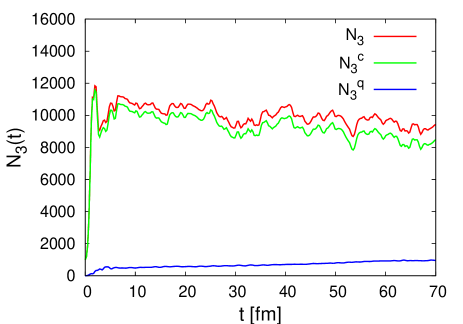
Figure 7: (Color online) Time evolution of the total particle numbers of the third component of pion field $N_{3}$, its classical part $N_{3}^{cl}$, and its quantum part $N_{3}^{q}$ in case ii(b).

Then, the expectation value of the particle number operator of the pion with isospin $a$ in the squeezed state is given as follows:

$$n_{a}({\vec{k}},t) = \langle\Phi(t)|{\hat{a}}_{a}^{\dagger}({\vec{k}}){\hat{a}}_{a}({\vec{k}})|\Phi(t)\rangle$$

$$= n_{a}^{cl}({\vec{k}},t)+n_{a}^{q}({\vec{k}},t),$$

$$n_{a}^{cl}({\vec{k}},t) = \frac{\omega_{k}}{2}C_{a}^{*}({\vec{k}},t)C_{a}({\vec{k}},t)+\frac{1}{2\omega_{k}}D_{a}^{*}({\vec{k}},t)D_{a}({\vec{k}},t)$$

$$- \frac{i}{2}\bigl{(}C_{a}^{*}({\vec{k}},t)D_{a}({\vec{k}},t)-C_{a}({\vec{k}},t)D_{a}^{*}({\vec{k}},t)\bigr{)},$$

$$n_{a}^{q}({\vec{k}},t) = \frac{\omega_{k}}{2}G_{aa}({\vec{k}},{\vec{k}},t)$$ (14)

$$+ \frac{1}{2\omega_{k}}\bigl{(}\frac{1}{4}G_{aa}^{-1}({\vec{k}},{\vec{k}},t)+4\langle{\vec{k}}|\Pi_{aa}G_{aa}\Pi_{aa}|{\vec{k}}\rangle\bigr{)}$$

$$+ i\langle{\vec{k}}|(G_{aa}\Pi_{aa}-\Pi_{aa}G_{aa})|{\vec{k}}\rangle,$$

where we have divided $n_{a}({\vec{k}},t)$ into the classical part $n_{a}^{cl}({\vec{k}},t)$ and the quantum part $n_{a}^{q}({\vec{k}},t)$; $n_{a}^{cl}({\vec{k}},t)$ includes the mean field and its time derivative, $C_{a}({\vec{k}},t)$ and $D_{a}({\vec{k}},t)$, and $n_{a}^{q}({\vec{k}},t)$ includes the quantities associated with the quantum fluctuation. On the right hand side of Eq. (14), no sum over $a$ is taken. In particular, no off-diagonal quantity with regard to the isospin indices appear on the right hand side of the last equation of (14) because no isospin-isospin correlation exists in either case ii(a) or case ii(b). In addition, we define the total particle numbers as the sum of the particle numbers over all modes,

$$N_{a}(t) = \sum_{{\vec{k}}}n_{a}({\vec{k}},t),$$

$$N_{a}^{cl}(t) = \sum_{{\vec{k}}}n_{a}^{cl}({\vec{k}},t),$$

$$N_{a}^{q}(t) = \sum_{{\vec{k}}}n_{a}^{q}({\vec{k}},t).$$ (15)

We have calculated these particle numbers by taking the ensemble average over 10 different initial field configurations. Figs. 6 and 7 show the time evolution of $N_{3}(t)$, $N_{3}^{cl}(t)$, and $N_{3}^{q}(t)$ in cases ii(a) and ii(b), respectively.

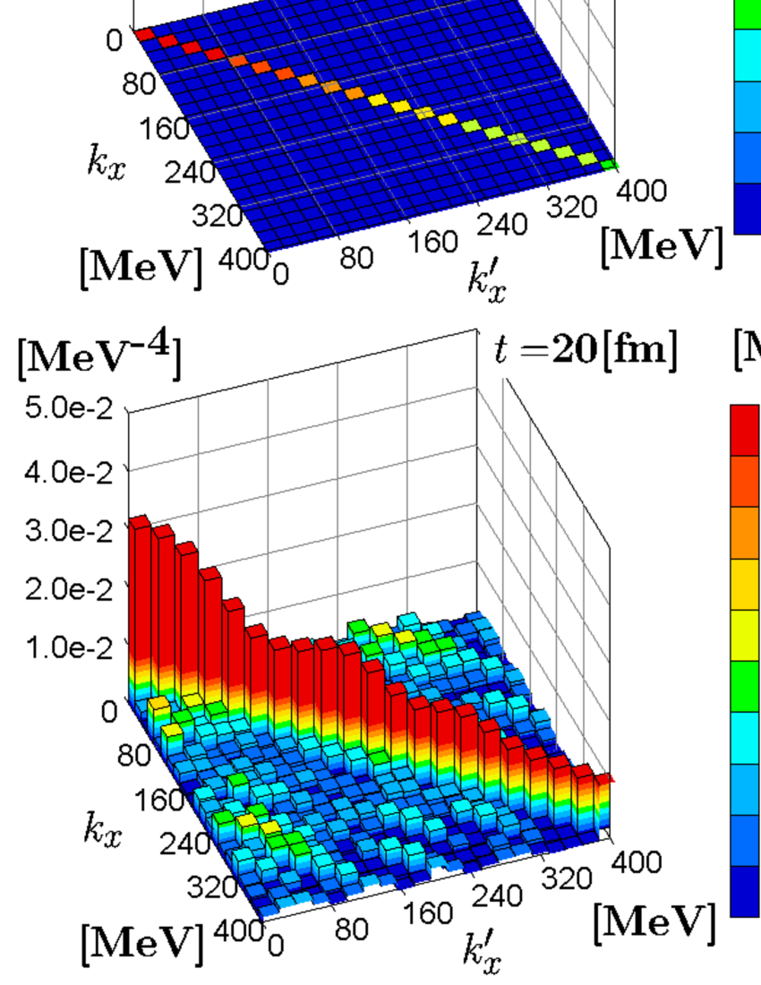
Figure 8: (Color online) Snap shots of the two-point function in momentum space, $|G_{33}({\vec{k}},{\vec{k}^{\prime}},t)|$, in case i(a). Note that the scale of the color legend at the initial time $t=0$ is different from the others.

We observe that the total particle number $N_{3}(t)$ rapidly increases within the typical time scale of the rolling-down of the order parameters (a few fm) in both cases. At first, the classical part $N_{3}^{cl}(t)$ is dominant in both cases. In case ii(a), where the mode-mode correlation is included, the classical part $N_{3}^{cl}(t)$ begins to decrease and the quantum part $N_{3}^{q}(t)$ begins to increase after a few fm, while the sum remains almost unchanged. The typical time scale of the increase of the quantum part is again close to that of the formation of the long range correlation. This clear separation of the stages in the time evolution of $N_{3}^{cl}(t)$ and $N_{3}^{q}(t)$ also shows that the main mechanism for the domain formation is not the rolling-down of the sigma field and the associated instability of pion fields with low momenta. On the other hand, in case ii(b), where less correlation results, the classical part of the total particle number $N_{3}^{cl}(t)$ is dominant throughout the time evolution.

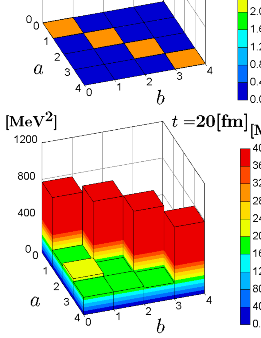
Figure 9: (Color online) Snap shots of the two-point function in isospin space, $\langle|G_{ab}(t)|\rangle$, in case i(a). Note that the scale of the color legend at the initial time $t=0$ is different from the others.

III.6 Off-diagonal components of the two-point functions in momentum space and isospin space

In this subsection, we show the time evolution of the off-diagonal components of the two-point functions in momentum space and also in isospin space, which correspond to the mode-mode correlation and isospin-isospin correlation, respectively.

Figure 8 shows the absolute value of the two-point function within the third component of the pion field in momentum space, $|G_{33}({\vec{k}},{\vec{k}^{\prime}},t)|$, in case i(a). In Fig. 8, no event average is taken. As explained in Section II, in general cases where there is no translational invariance, the off-diagonal components of the two-point functions develop and grow as the system evolves in time even if they are initially absent. According to Fig. 8, the off-diagonal components indeed appear as time elapses. Although the diagonal components are always dominant, the off-diagonal components are not negligible, in particular, at low momenta. This existence of the off-diagonal components is crucial for the DCC formation and the evolution of the quantum fluctuation, as we have already demonstrated.

Figure 9 represents the time evolution of the two-point functions in isospin space in case i(a). In this figure, the spatial average of their absolute value,

$$\langle|G_{ab}(t)|\rangle=\frac{1}{V}\int|G_{ab}({\vec{x}},{\vec{x}},t)|d{\vec{x}},$$ (16)

is shown. No event average is taken in Fig. 9, either. At the initial time, the two-point function is diagonal in isospin space as in momentum space. The off-diagonal components of the two-point function emerge and develop as time elapses. The absolute value of the off-diagonal components evolves up to about one fourth of that of the diagonal components by $t\sim 25$ fm, and then their relative strength starts to decrease.

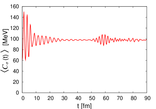
Figure 10: (Color online) Time evolution of the spatial average of the sigma field.

III.7 Dissipation of the sigma field

Finally, we explore whether and how the dissipation of the sigma field is included in the approximation. For this purpose, we chose the following initial condition. The mean field of the sigma field $C_{0}$ was randomly distributed according to the same Gaussian form as Eq. (9) except that the first equation was replaced by $\langle C_{0}\rangle=60$ MeV. The pion fields and their conjugate fields were set to zero at each lattice point. As for the quantum fluctuation and correlation, the same initial condition as in Section II.2, i.e., those of independent coherent states with the degenerate mass $m_{0}=200$ MeV, were used. Ensemble average was taken over 10 initial configurations as before. In the calculation, both mode-mode and isospin-isospin correlations are taken into account, i.e., case i(a).

Figure 10 represents the time evolution of the spatial average of the mean field part of the sigma field. The result tells us that the oscillation of the sigma field is damped quickly and it approaches a constant. Since initially the pion fields and their conjugate variables are all zero, the mean field part of the pion fields remains zero throughout the time evolution. On the contrary, the quantum fluctuation of the pion fields is not zero initially and, moreover, it is amplified substantially as shown for the third component in Fig. 11, while that of the sigma field changes only little. This amplification does not exist in the translationally invariant case. Physically, the damping of the oscillation of the sigma field and the growth of the quantum fluctuation of the pion fields correspond to the decays of the sigma into two pions. As observed from Figs. 10 and 11, the growth of the fluctuation of the pion fields stops approximately at the same time as the oscillation of the sigma fields ends.

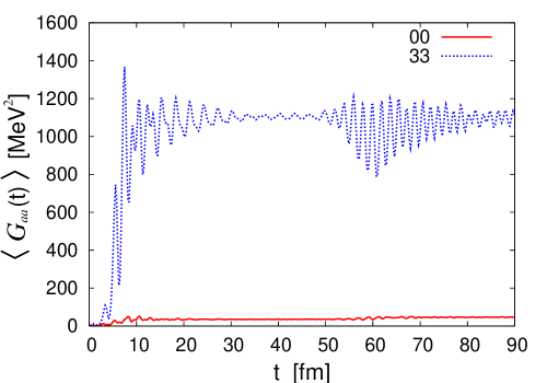
Figure 11: (Color online) Time evolution of the quantum fluctuation of the sigma field (00) and the third component of the pion field (33).

IV Conclusion

In this paper, we have studied the dynamics of chiral phase transition in spatially inhomogeneous systems with mode-mode correlations in the framework of TDVA with squeezed states for the 1+1 dimensional geometry. Quantum effects and spatial inhomogeneity are both incorporated.

In the case with the mode-mode correlation, the DCC domain formation continues beyond the time scale of the rolling-down of the order parameter. The quantum fluctuation is also amplified with approximately the same time scale. This implies that squeezing of the states takes place. On the other hand, no significant DCC domain formation or squeezing of the states was observed in the case without the mode-mode correlation. Thus, it is concluded that the mode-mode correlation plays the key role in the formation of DCC domain. This mode-mode correlation has not been taken into account in preceding quantum calculations for DCC formation. In addition, it was pointed out that this mechanism is different from the previously proposed parametric resonance amplification.

We have also examined the effect of the isospin-isospin correlation on the domain formation of DCC for the first time. We found that the isospin-isospin correlation makes the DCC domain structure larger, but its effect is less conspicuous than that of the mode-mode correlation. The isospin-isospin correlation has almost negligible effects on the time evolution of the quantum fluctuation. Thus, the isospin-isospin correlation does not lead to further squeezing of the states.

We plan to include realistic geometry and dynamics such as expansion, and carry out calculations in 2+1 or 3+1 dimension in future work. They are indispensable for the quantum mechanical understanding of the DCC formation in ultra-relativistic heavy ion collisions.

- (1) K. Rajagopal and F. Wilczek, Nucl. Phys. B404, 577 (1993).
- (2) M. Asakawa, Z. Huang, and X.-N. Wang, Phys. Rev. Lett. 74, 3126 (1995).
- (3) D. Boyanovsky, H. J. de Vega, and R. Holman, Phys. Rev. D 49, 2769 (1994); D. Boyanovsky, H. J. de Vega, R. Holman, D. S. Lee, and A. Singh, Phys. Rev. D 51, 4419 (1995); D. Boyanovsky, H. J. de Vega, R. Holman, and J. Salgado, Phys. Rev. D 59, 125009 (1999).
- (4) F. Cooper, S. Habib, Y. Kluger, E. Mottola, J. P. Paz, and P. R. Anderson, Phys. Rev. D 50, 2848 (1994); F. Cooper, Y. Kluger, E. Mottola, and J. P. Paz, Phys. Rev. D 51, 2377 (1995).
- (5) F. Cooper, J. F. Dawson, and B. Mihaila, Phys. Rev. D 67, 056003 (2003).
- (6) M. Salle, J. Smit, and J. C. Vink, Phys. Rev. D 64, 025016 (2001); M. Salle, J. Smit, and J. C. Vink Nucl. Phys. B625, 495 (2002); G. Aarts and J. Smit, Phys. Rev. D 61, 025002 (2001).
- (7) L. M. A. Bettencourt, K. Pao and J. G. Sanderson, Phys. Rev. D 65, 025015 (2002).
- (8) J. Berges, Nucl. Phys. A699, 847 (2002); G. Aarts, D. Ahrensmeier, R. Baier, J. Berges, and J. Serreau, Phys. Rev. D 66, 045008 (2002).
- (9) T. Ikeda, Phys. Rev. D 69, 105018 (2004).
- (10) N. Ikezi, M. Asakawa and Y. Tsue, Phys. Rev. C 69, 032202(R) (2004).
- (11) R. Jackiw and A. Kerman, Phys. Lett. A71, 158 (1979).
- (12) Y. Tsue and Y. Fujiwara, Prog. Theor. Phys. 86, 443 (1991); Prog. Theor. Phys. 86, 469 (1991).
- (13) Y. Tsue, A. Koike, and N. Ikezi, Prog. Theor. Phys. 106, 469 (2001) 807.
- (14) M. Asakawa, H. Minakata, and B.Müller, Phys. Rev. D 58, 094011 (1998).
- (15) S. Gavin and B. Muller, Phys. Lett. B329, 486 (1994).
- (16) S. Mrówczyński and B. Müller, Phys. Lett. B 363, 1 (1995).