Effects of $\beta$-$\gamma$ coupling in transitional nuclei and the validity of the approximate separation of variables

Abstract

Exact numerical diagonalization is carried out for the Bohr Hamiltonian with a $\beta$-soft, axially stabilized potential. Wave function and observable properties are found to be dominated by strong $\beta$-$\gamma$ coupling effects. The validity of the approximate separation of variables introduced with the $\mathrm{X}(5)$ model, extensively applied in recent analyses of axially stabilized transitional nuclei, is examined, and the reasons for its breakdown are analyzed.

I Introduction

The Bohr Hamiltonian bohr1998:v2 with a $\beta$-soft but $\gamma$-stabilized potential has served as the basis of recent investigations of the collective structure of transitional nuclei intermediate between spherical and axially symmetric deformed shape iachello2001:x5. The solutions obtained so far for the $\mathrm{X}(5)$ model iachello2001:x5; bijker2003:x5-gamma and its various extensions bonatsos2004:x5-monomial; caprio2004:swell; bonatsos2004:z5-triax; fortunato2004:beta-soft-triax; pietralla2004:confined-beta-soft; bonatsos2005:octupole-aqoa-actinides have relied upon an approximate separation of variables, introduced in Ref. iachello2001:x5, since solution of the exact problem was not possible. These approximate calculations have been extensively compared with experimental data casten2001:152sm-x5; bizzeti2002:104mo-x5; kruecken2002:150nd-rdm; caprio2002:156dy-beta; dewald2002:150nd-rdm; caprio2003:diss; hutter2003:104mo106mo-rdm; clark2003:x5-search; tonev2004:154gd-rdm; mccutchan2004:162yb-beta; mccutchan2005:166hf-beta.

However, numerical methods recently developed by Rowe et al. rowe2004:tractable-collective; rowe2004:spherical-harmonics; rowe2005:collective-algebraic make exact numerical diagonalization of the Bohr Hamiltonian feasible for transitional and deformed situations, without recourse to the approximations of Ref. iachello2001:x5. The solution process involves diagonalization in a basis constructed from products of optimally chosen $\beta$ wave functions with five-dimensional spherical harmonics. This method yields much more rapid convergence in the presence of significant $\beta$ deformation than is obtained with conventional methods gneuss1971:gcm; eisenberg1987:v1.

In the present work, an exact numerical solution for the $\mathrm{X}(5)$ Hamiltonian is obtained (Sec. II). The results for wave functions and observables are examined, and the properties of $\beta$-soft nuclei are found to be dominated by a strong coupling between the $\beta$ and $\gamma$ degrees of freedom (Sec. III). Since extensive prior work has been carried out using the approximate separation of variables of Ref. iachello2001:x5, this approximation is reviewed and the reasons for its breakdown are analyzed (Sec. IV).

II Hamiltonian and solution method

Figure 1: Simple forms of the potential $V_{\gamma}(\gamma)$ satisfying the coordinate symmetry constraints of Ref. eisenberg1987:v1: (a) $V_{\gamma}(\gamma)=\chi(1-\cos 3\gamma)$ rowe2004:tractable-collective and (b) $V_{\gamma}(\gamma)=A\gamma^{2}$ ($0\leq\gamma\leq\pi/3$), used here for consistency with Ref. iachello2001:x5.

The Bohr Hamiltonian, in terms of the quadrupole deformation variables $\beta$ and $\gamma$ and the Euler angles $\vartheta$, is bohr1998:v2

$$H=-\frac{\hbar^{2}}{2B}\Biggl{[}\frac{1}{\beta^{4}}\frac{\partial}{\partial\beta}\beta^{4}\frac{\partial}{\partial\beta}+\frac{1}{\beta^{2}}\left(\frac{1}{\sin 3\gamma}\frac{\partial}{\partial\gamma}\sin 3\gamma\frac{\partial}{\partial\gamma}-\frac{1}{4}\sum_{\kappa}\frac{\hat{L}_{\kappa}^{\prime 2}}{\sin^{2}(\gamma-\frac{2}{3}\pi\kappa)}\right)\Biggr{]}+V(\beta,\gamma),$$ (1)

where $\hat{L}_{\kappa}^{\prime}$ are the intrinsic frame angular momentum components. For the transition between spherical and axially symmetric deformed structure, it is appropriate to consider a potential $V(\beta,\gamma)$ which is soft with respect to $\beta$ but which provides confinement about $\gamma=0$. In the $\mathrm{X}(5)$ model, a schematic form $V(\beta,\gamma)=V_{\beta}(\beta)+V_{\gamma}(\gamma)$ is used, where $V_{\beta}$ is taken to be a square well potential [$V_{\beta}(\beta)=0$ for $\beta\leq\beta_{w}$ and $\infty$ otherwise] and $V_{\gamma}$ provides stabilization around $\gamma=0$.

Under the approximate separation of variables of Ref. iachello2001:x5, most results are independent of the specific choice of $V_{\gamma}$. Consequently, in Ref. iachello2001:x5, the confining potential $V_{\gamma}(\gamma)$ is simply described as $\propto\gamma^{2}$ for small $\gamma$. For solution of the full problem, $V_{\gamma}(\gamma)$ must be defined more completely. In general for the Bohr Hamiltonian, the potential energy $V(\beta,\gamma)$ must be periodic in $\gamma$, with period $2\pi/3$, and reflection symmetric about $\pi/3$, to ensure that the potential energy is invariant under relabeling of the intrinsic axes eisenberg1987:v1. The natural choice of such potential is $V_{\gamma}(\gamma)\propto(1-\cos 3\gamma)$ [Fig. 1(a)], as considered in Ref. rowe2004:tractable-collective. However, for consistency with Ref. iachello2001:x5, in the present work the $\gamma$ potential is chosen to be the oscillator potential, given by $V_{\gamma}(\gamma)=A\gamma^{2}$ on the interval $0\leq\gamma\leq\pi/3$ and obtained outside this interval from the symmetry requirements on $\gamma$ [Fig. 1(b)].

As usual for eigenproblems involving the Bohr Hamiltonian, the parameter dependence of the solution can be simplified by an appropriate choice of dimensionless parameters. Transformation of the potential as $V(\beta,\gamma)\rightarrow c^{2}V(c\beta,\gamma)$ or multiplication of the Hamiltonian by a constant factor both leave the solution invariant, to within an overall scale factor on the eigenvalues and an overall dilation of all wave functions (e.g., Ref. caprio2003:gcm). Consequently, all energy ratios and transition matrix elements obtained from diagonalization of the Hamiltonian (1) depend only upon the parameter combination

$$a\equiv\frac{2AB\beta_{w}^{2}}{\hbar^{2}},$$ (2)

which measures the “$\gamma$-stiffness” of the Hamiltonian. In the remainder of this article, the notation is simplfied by setting $\hbar^{2}/(2B)=1$ and $\beta_{w}=1$, so that $a=A$. (Results for any other values of these parameters may then be obtained according to simple scaling relations caprio2003:gcm.)

For $a=0$, the potential is $\gamma$-independent, and the Hamiltonian (1) reduces to the $\mathrm{E}(5)$ Hamiltonian iachello2000:e5. In this case, an exact separation of variables occurs wilets1956:oscillations, and the eigenproblem can be solved analytically iachello2000:e5. Nonzero values of $a$ yield confinement around $\gamma=0$. The realistic range of values for $a$ is discussed in Sec. III.

Rowe et al. rowe2004:tractable-collective; rowe2004:spherical-harmonics; rowe2005:collective-algebraic have recently proposed a method for numerical diagonalization of the Bohr Hamiltonian, with respect to an optimized product basis constructed from the five-dimensional spherical harmonics bes1959:gamma; santopinto1996:so-brackets. Much as a basis for solution of the Schrödinger problem in three dimensions can be formed from the products of a complete set of radial functions $f_{i}(r)$ with the three-dimensional spherical harmonics $Y^{L}_{M}(\theta,\varphi)$, a basis for solution of the Bohr problem can be constructed from products of radial basis functions $f_{i}(\beta)$ with the five-dimensional spherical harmonics $\Psi_{v\alpha{}LM}(\gamma,\vartheta)$.

This method is especially suitable for application to transitional and deformed nuclei, since the radial basis functions can be chosen to match the particular radial potential at hand. It provides vastly more rapid convergence in the presence of significant $\beta$ deformation than is obtained with conventional methods based on diagonalization in an oscillator basis (see Ref. rowe2005:collective-algebraic). Also, it can be applied to potentials for which the oscillator basis methods are simply inapplicable. For the $\mathrm{X}(5)$ problem, the wave functions must vanish for $\beta>1$. This boundary condition cannot be satisfied in a finite basis of oscillator eigenfunctions. Instead, in the present work suitable basis functions are defined as $f_{i}(\beta)\propto\beta^{-3/2}J_{\nu}(x_{\nu,i}\beta)$ for $\beta\leq 1$ and zero elsewhere, where $x_{\nu,i}$ is the $i$th zero of $J_{\nu}$. The calculation of Hamiltonian matrix elements with respect to this radial basis is described further in the Appendix. The choice $\nu=3/2$ makes these $f_{i}(\beta)$ the exact radial wave functions for the seniority zero states in the $\mathrm{E}(5)$ limit ($a=0$) iachello2000:e5.

Rowe et al. rowe2004:spherical-harmonics provide an algorithm for the explicit construction of the five-dimensional spherical harmonics, as sums of the form $\Psi_{v\alpha{}LM}(\gamma,\vartheta)=\sum_{\begin{subarray}{c}K=0\\ \text{even}\end{subarray}}^{L}F_{v\alpha{}LK}(\gamma)\phi^{L}_{MK}(\vartheta)$, where $\phi^{L}_{MK}(\vartheta)\equiv[(2L+1)/(16\pi^{2}(1+\delta_{K}))]^{1/2}[D^{L}_{MK}(\vartheta)+(-)^{L}D^{L}_{M-K}(\vartheta)]^{*}$. The spherical harmonics are seniority eigenstates, labeled by the seniority quantum number $v$, a multiplicity index $\alpha$, and the angular momentum quantum numbers $L$ and $M$. They are the exact angular wave functions in the $\gamma$-soft ($a=0$) limit of the present problem. In the Hamiltonian (1), the angular kinetic energy operator (the quantity in parentheses) is simply the negative of the seniority operator $\hat{\Lambda}$ wilets1956:oscillations. Thus, calculation of its matrix elements between spherical harmonics is trivial (LABEL:eqngammakeme). The matrix elements of an arbitrary spherical tensor function of $\gamma$ and the Euler angles can be obtained through a series of straightforward integrations, as detailed further in the Appendix.

High-seniority spherical harmonics are needed for the construction of highly $\gamma$-localized wave functions. Thus, in general, diagonalization for larger $\gamma$-stiffnesses requires larger angular bases. For the range of $\gamma$ stiffnesses considered in the present work ($0\leq a\leq 1000$), a product basis constructed from the first $\sim 5$ radial functions and the $15$ to $20$ lowest seniority spherical harmonics suffices to provide convergence of the calculated observables for low-lying states.

III Results

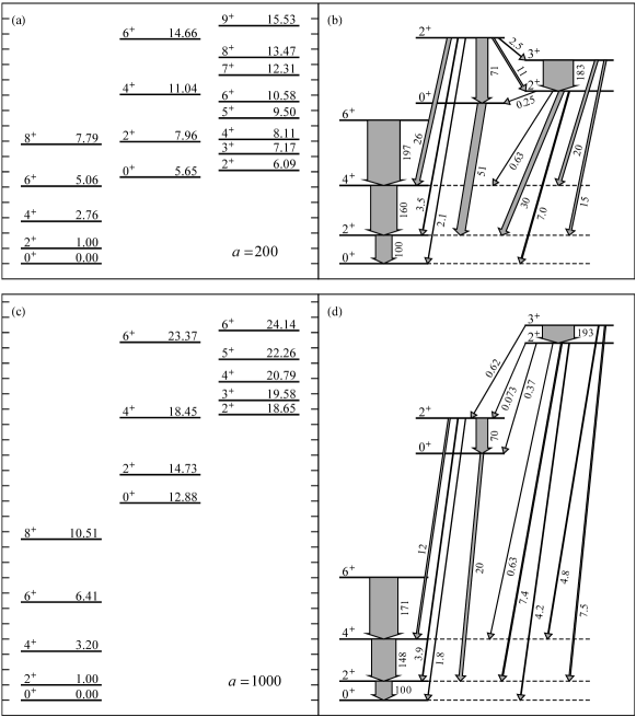
Figure 2: Level schemes for $a=200$ (top) and $a=1000$ (bottom), from the exact numerical solution for the $\mathrm{X}(5)$ Hamiltonian. Excitation energies of the lowest members of the ground, $\beta$, and $\gamma$ bands, normalized to $E(2^{+}_{1})$, are shown at left. Electric quadrupole transition strengths, normalized to $B(E2;2^{+}_{1}\rightarrow 0^{+}_{1})=100$, are shown at right.

Figure 3: Contour plots of the probability distributions with respect to $\beta$ and $\gamma$, from the exact numerical solution for the $\mathrm{X}(5)$ Hamiltonian, for (top) the ground state ($0^{+}_{1}$), (middle) the $\beta$ band head ($0^{+}_{\beta}$), and (bottom) the $\gamma$ band head ($2^{+}_{\gamma}$). These are shown for $\gamma$ stiffness parameter values $a=0$ (left), $a=200$ (middle), and $a=1000$ (right). Contours of the potential [$V_{\gamma}(\gamma)=a\gamma^{2}$] are also shown (dashed curves). For the $\gamma$-soft case $a=0$, where the bands are not well defined, the $0^{+}_{1}$ ($\xi=1$, $v=0$), $0^{+}_{2}$ ($\xi=2$, $v=0$), and $2^{+}_{2}$ ($\xi=1$, $v=2$) states, respectively, are shown. Plots are in the standard polar form, with $\beta$ as the radial coordinate and $\gamma$ as the angular coordinate.

Figure 4: Probability distributions with respect to $\beta$ (left) and $\gamma$ (right) for the ground state (solid), the $\beta$ band head (dashed), and the $\gamma$ band head (dotted), shown for $\gamma$ stiffness parameter values (top) $a=0$, (middle) $a=200$, and (bottom) $a=1000$. The $\gamma$-confining potential $V_{\gamma}$ and the level eigenvalues are shown in the insets. In panel (b), as in Fig. 3, the $0^{+}_{1}$ ($\xi=1$, $v=0$), $0^{+}_{2}$ ($\xi=2$, $v=0$), and $2^{+}_{2}$ ($\xi=1$, $v=2$) states are shown. These states have identical $\gamma$ distributions, $P(\gamma)\propto\sin 3\gamma$.

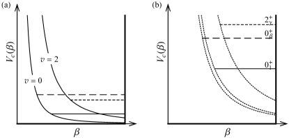
Figure 5: (a) Centrifugal potentials $V_{c}(\beta)=(v+1)(v+2)/\beta^{2}$ for the radial Schrödinger equation in the $\gamma$-soft limit, for quantum numbers $v=0$ and $2$. (b) Effective centrifugal potentials $V_{c}(\beta)=\langle(v+1)(v+2)\rangle/\beta^{2}$, schematically indicating the strength of the centrifugal effect for the $\gamma$-stabilized case $a=1000$. The level energies and centrifugal potentials are shown for the same states as in Figs. 3 and 4, namely, the ground state (solid), the $\beta$ band head (dashed), and the $\gamma$ band head (dotted).

Figure 6: Dependence of energy observables upon the $\gamma$ stiffness parameter $a$, for $0\leq a\leq 1000$. (a) Excitation energies of the $0^{+}_{2}$ (solid), $2^{+}_{2}$ and $2^{+}_{3}$ (dashed), and $3^{+}_{1}$ (dotted) levels, normalized to $E(2^{+}_{1})$. For large $a$, these states become the lowest spin members of the $\beta$ and $\gamma$ bands. (b) Energy ratio $R_{4/2}\equiv E(4^{+}_{1})/E(2^{+}_{1})$.

Figure 7: Dependence of $B(E2)$ observables upon the $\gamma$ stiffness parameter $a$, for $0\leq a\leq 1000$. (a) Branches from the $2^{+}_{2}$ level to the yrast $0^{+}$ (solid), $2^{+}$ (dashed), and $4^{+}$ (dotted) levels, normalized to $BE(2^{+}_{1}\rightarrow 0^{+}_{1})$. Immediately below the avoided crossing at $a\approx 450$ this is the $2^{+}_{\gamma}$ level, while immediately above it is the $2^{+}_{\beta}$ level (as indicated). (b) Branches from the $2^{+}_{3}$ level to the yrast $0^{+}$ (solid), $2^{+}$ (dashed), and $4^{+}$ (dotted) levels, normalized to $BE(2^{+}_{1}\rightarrow 0^{+}_{1})$. Immediately below the avoided crossing at $a\approx 450$ this is the $2^{+}_{\beta}$ level, while immediately above it is the $2^{+}_{\gamma}$ level (as indicated).

Figure 8: Yrast band (a) energies and (b) $B(E2)$ strengths as functions of angular momentum, for $a=0$, $200$, and $1000$ (dashed). The values obtained under the approximate separation of variables (Sec. IV) are indicated for reference, as are the rigid rotor values (solid).

Results obtained from numerical diagonalization of the $\mathrm{X}(5)$ Hamiltonian, for $a=200$ and $a=1000$, are shown in Fig. 2. Level energies and $E2$ transition strengths for the lowest-lying levels are indicated. More detailed tabulations of energy and $B(E2)$ observables, calculated for $0\leq a\leq 1000$, are provided through the Electronic Physics Auxiliary Publication Service (EPAPS) axialsep-epaps. For the transitional rare earth nuclei (with $N\approx 90$) the $\gamma$ band head energy is $\sim 6$ to $8$ times the $2^{+}_{1}$ energy, consistent with a $\gamma$ stiffness $a\approx 200$ to $300$. This may therefore be considered the most “realistic” range of values for the $\gamma$ stiffness parameter, of the greatest phenomenological interest.

First let us note some basic properties of the solution [Fig. 2]. The levels are organized into clearly-defined bands, characterized by strong intraband transition strengths. The lowest energy bands have the spin contents associated with a rotational ground state band, $\beta$ band, and $\gamma$ band. From a comparison of the $a=200$ and $a=1000$ cases shown in Fig. 2, it is apparent that such properties as the band head excitation energies, energy spacings within the bands, and transition strengths are strongly dependent on the $\gamma$ stiffness. This is true for both the $\beta$ and $\gamma$ bands. While it is natural to expect the $\gamma$ band energy to increase with $\gamma$ stiffness, it is seen from Fig. 2 that the $\beta$ band head energy also increases with $\gamma$ stiffness by a comparable amount. For larger $\gamma$ stiffness [Fig. 2(c)], the energy spacings within the bands tend towards rigid rotor [$L(L+1)$] spacings.

Before considering the spectroscopic observables in greater detail, let us first examine the underlying features of the wave functions $\varphi(\beta,\gamma,\vartheta)$. In the approximate treatments of the problem iachello2001:x5, the wave functions were separable into products of $\beta$, $\gamma$, and Euler angle functions, which were considered separately. This is no longer possible for the full solutions, but we can still consider the probability distributions with respect to one or more of these coordinates, constructed by integration over all remaining coordinates (see Appendix). The integration metric appropriate to the Bohr coordinates is $\beta^{4}d\beta\lvert\sin 3\gamma\rvert d\gamma d\vartheta$ bohr1998:v2; eisenberg1987:v1. Contour plots of the probability distribution with respect to $\beta$ and $\gamma$ are shown in Fig. 3, for the ground, $\beta$, and $\gamma$ band head states. The probability distributions with respect to $\beta$ or $\gamma$ individually, i.e., integrated over the other coordinate, are shown for these same states in Fig. 4.

The $\gamma$ dependences of the probability distributions of the various states [Figs. 3 and 4 (right)] are modulated by the $\lvert\sin 3\gamma\rvert$ factor in the integration metric, which causes the probability density to vanish at $\gamma=0$ and $\pi/3$. In the $\gamma$-soft limit, the probability distributions for several of the lowest-lying states are simply $P(\gamma)\propto\sin 3\gamma$ [Fig. 4(b)] and thus peaked at $\gamma=\pi/6$, or $30^{\circ}$. For the $\gamma$-stabilized cases [Fig. 4(d,f)], the $\gamma$ distributions for the $0^{+}_{1}$ and $0^{+}_{\beta}$ states are similar to each other, while that for the $2^{+}_{\gamma}$ state is peaked at nearly twice the $\gamma$ value. The probability distributions are compressed closer to $\gamma=0$ with increasing Hamiltonian $\gamma$-stiffness, but even for the stiffest case considered ($a=1000$) the value of $\langle\gamma\rangle$ is $\sim 11^{\circ}$ for the ground state and $\sim 16^{\circ}$ for the $\gamma$ band head.

Thus, for realistic $\gamma$ stiffnesses, the wave functions exhibit considerable “dynamical” $\gamma$ softness. This is perhaps contrary to the common conception that nuclei with well-defined $\gamma$-bands, like those in Fig. 2, are “axially symmetric” and have $\gamma\approx 0$. (Recent empirical estimates of the effective $\gamma$ deformation of transitional and deformed rare earth nuclei werner2005:triax-invariant yield comparably large dynamical $\gamma$ softness.)

The $\beta$ dependences of the probability distributions of the various states [Figs. 3 and 4 (left)] are seen to be strongly influenced by $\beta$-$\gamma$ interaction, migrating towards larger $\beta$ as the $\gamma$ stiffness increases. This evolution can be understood in a qualitative fashion in terms of the five-dimensional analogue of the centrifugal effect. In the $\gamma$-soft limit, where the problem is separable, the $\beta$ wave function is governed by a radial Schrödinger equation containing a term $V_{c}(\beta)=(v+1)(v+2)/\beta^{2}$ wilets1956:oscillations; rakavy1957:gsoft, analogous to the centrifugal potential in the three-dimensional central force problem, as shown in Fig. 5(a). The strength of this term depends upon the seniority quantum number $v$, alternatively denoted $\tau$ in Ref. iachello2000:e5. The $1/\beta^{2}$ dependence energetically penalizes small $\beta$ values and tends to “push” the wave function towards larger $\beta$. But even in the $\gamma$-stabilized situation, an analogue of the centrifugal effect occurs, and its general features may be understood by observing that the angular kinetic energy operator [the factor in parentheses in the Hamiltonian (1)] multiplies a $\beta$-dependent factor $1/\beta^{2}$. The angular kinetic energy contains contributions from both the rotational degrees of freedom and the $\gamma$ degree of freedom. As the $\gamma$ stiffness of the potential increases, the confinement about $\gamma=0$ results in a larger $\gamma$ contribution to kinetic energy, even for the ground state, where this is essentially the $\gamma$ vibrational zero point kinetic energy. Thus, as the $\gamma$ stiffness increases, the influence of the $1/\beta^{2}$ term in the Hamiltonian becomes larger, displacing the wave functions towards larger $\beta$.

An idea of the strength of the centrifugal effect in the $\gamma$-stabilized cases can be obtained by numerically evaluating the expectation value of the angular kinetic energy for any given state. The resulting “effective” centrifugal potential $V_{c}(\beta)=\langle(v+1)(v+2)\rangle/\beta^{2}=\langle\hat{\Lambda}+2\rangle/\beta^{2}$ is shown in Fig. 5(b). (This potential is not of calculational value, but it is useful in understanding the solution properties.) For the square well $\beta$ potential used in the present model, the extent of the wave function in $\beta$ is limited by the hard wall at $\beta=1$. The centrifugal effect compresses the wave function against the wall, so for large $\gamma$ stiffnesses the wave function becomes localized with respect to $\beta$, just within the wall. Thus, even though the potential is flat in $\beta$, the $\beta$-$\gamma$ interaction inherent in the kinetic energy operator induces something akin to rigid $\beta$ deformation.

The $0^{+}_{\beta}$ state has a bimodal probability distribution with respect to $\beta$ [Fig. 4 (left)]. In the $\gamma$-soft limit [Fig. 4(a)], an exact zero in the probability distribution arises from the node in the radial wave function, but for $a>0$ an exact zero is not expected. The $0^{+}_{\beta}$ state also has a smaller mean value of $\beta$ than the ground state. The $0^{+}_{\beta}$ state is subject to a similar effective centrifugal potential to that for the ground state [Fig. 5(b)], but it has more energy available in the $\beta$ degree of freedom and is thus less strongly confined against the wall at $\beta=1$. The $2^{+}_{\gamma}$ state instead has a larger mean $\beta$ than the ground state. The angular kinetic energy for the $\gamma$ band is about twice that for the ground state, in the limit of harmonic $\gamma$ oscillations iachello2001:x5, and hence so is the centrifugal effect [Fig. 5(b)]. For $a=200$ the mean $\beta$ values are $\langle\beta\rangle_{0^{+}_{1}}\approx 0.64$, $\langle\beta\rangle_{0^{+}_{\beta}}\approx 0.54$, and $\langle\beta\rangle_{2^{+}_{\gamma}}\approx 0.70$, while for $a=1000$ they are $\langle\beta\rangle_{0^{+}_{1}}\approx 0.71$, $\langle\beta\rangle_{0^{+}_{\beta}}\approx 0.60$, and $\langle\beta\rangle_{2^{+}_{\gamma}}\approx 0.76$.

The dependences of a few basic observables upon the $\gamma$ stiffness are shown in Figs. 6–8. Naturally, the $\gamma$ band energy increases with $\gamma$ stiffness: the evolution proceeds from the $\mathrm{E}(5)$ limit ($a=0$), through $\gamma$ excitation energies appropriate to rare earth transitional nuclei ($a\approx 200$ to $300$), to very $\gamma$-stiff structure [Fig. 6(a)]. But the $\beta$ excitation energy increases with $\gamma$ stiffness as well, at about half the rate at which the $\gamma$ excitation energy does. An avoided crossing of the $2^{+}_{\beta}$ and $2^{+}_{\gamma}$ states occurs for $a\approx 450$.

The angular momentum dependence of energies within the yrast band varies substantially with $\gamma$ stiffness [Fig. 8(a)]. For large $a$, it approaches the $L(L+1)$ dependence of the axially symmetric rigid rotor. In particular, the energy ratio $R_{4/2}\equiv E(4^{+}_{1})/E(2^{+}_{1})$ ranges from $2.20$ in the $\mathrm{E}(5)$ limit to $\gtrsim 3.2$ for large $a$ [Fig. 6(b)]. The yrast band $B(E2)$ strengths [Fig. 8(b)] also vary with stiffness, for large $a$ likewise approaching rigid rotor values. The observables are thus seen to clearly reflect the rigid $\beta$ deformation induced by the centrifugal effect at large $\gamma$ stiffness.

Further inspection of Fig. 2 provides a more detailed view of the spectroscopic properties obtained. Strong interband $E2$ transitions are predicted, some comparable in strength to in-band transitions. A radical suppression of the spin-descending $\beta$ band to ground state band transitions (e.g., $2^{+}_{\beta}\rightarrow 0^{+}_{1}$) relative to the spin-ascending transitions (e.g., $2^{+}_{\beta}\rightarrow 4^{+}_{1}$) is one of the most notable features. (Only the branching of the $2^{+}_{\beta}$ state is shown in Fig. 2, but the branchings of the higher-spin band members are provided through the EPAPS axialsep-epaps.) The strengths of the interband transitions depend in detail upon the $\gamma$ stiffness, as shown in Fig. 7. As the $\gamma$ stiffness increases, the $\beta$ to ground band and $\gamma$ to ground band transitions become weaker overall. They also tend closer to the rigid rotor Alaga rule branching ratios bohr1998:v2. Strong $\beta$-$\gamma$ interband transition strengths occur as well [Fig. 2], but these vary greatly with $\gamma$ stiffness.

For all $\gamma$ stiffnesses, the energy spacing scale of the $\beta$ band is enlarged relative to that of the ground state band [Figs. 2 and 6(a)]. (In contrast, the spacing scale of levels within the $\gamma$ band is similar to that of the ground state band.) The enlarged spacing scale may be understood in terms of the $\beta$ probability distributions. For a rigid rotor, with fixed $\beta$, the spacing scale of levels within a band is proportional to $1/\beta^{2}$ bohr1998:v2. As observed above, the probability distribution of the $0^{+}_{\beta}$ state tends towards smaller $\beta$ than that of the ground state, giving a larger average $1/\beta^{2}$. The ratio $\langle\beta^{-2}\rangle_{0^{+}_{\beta}}/\langle\beta^{-2}\rangle_{0^{+}_{1}}$ has a maximum value of $\sim 2.1$ for $a\approx 200$ and decreases to $\sim 1.8$ for $a=1000$. Similarly, the ratio of spacing scales, $[E(2^{+}_{\beta})-E(0^{+}_{\beta})]/E(2^{+}_{1})$, has a maximum value of $\sim 2.3$ for $a\approx 200$ and decreases to $\sim 1.9$ for $a=1000$.

From this understanding of the underlying mechanism, it is seen that enlarged energy spacing scale of the $\beta$ band is an artifact of the rigid well wall in the $\mathrm{X}(5)$ Hamiltonian caprio2004:swell. As already noted, the extra energy available to the $\beta$ excitation, relative to the ground state, allows its wave function to expand “inward” against the centrifugal potential [Fig. 5(b)], but not “outward” against the rigid wall. This produces the larger $\langle\beta^{-2}\rangle$ and hence rotational energy scale for the $\beta$ excitation. A similar expanded spacing scale for the $\beta$ band is encountered in descriptions of transitional nuclei with the interacting boson model (IBM) scholten1978:ibm-u5-su3 and the geometric collective model (GCM) zhang1999:152sm-gcm. In these cases the potential wall is no longer rigid but rather quartic ($\propto\beta^{4}$), but the same basic mechanism may apply (see, e.g., Fig. 15.8 of Ref. caprio2003:diss).

Another distinctive feature of the exact solution is the staggering of energies within the $\gamma$ band, clearly visible for $a=200$ [Fig. 2(a)]. The level energies are clustered as $2^{+}(3^{+}4^{+})(5^{+}6^{+})\ldots$, contrary in sense to the $(2^{+}3^{+})(4^{+}5^{+})\ldots$ staggering of the rigid triaxial rotor davydov1958:arm-intro. The staggering is a remnant of the $\mathrm{SO}(5)$ multiplet structure wilets1956:oscillations; rakavy1957:gsoft present in the $\gamma$-soft limit ($a=0$) and is an observable manifestation of the considerable dynamical $\gamma$ softness seen in Fig. 4(d). It disappears with increasing $\gamma$ stiffness [Fig. 2(c)]. In general in a geometric description, a weakly $\gamma$-confining potential yields both dynamical $\gamma$-softness and a low $\gamma$ excitation energy, while a strongly $\gamma$-confining potential yields $\gamma$ localization and a high $\gamma$ excitation energy. Hence, the presence of signatures of $\gamma$ softness (such as the $\gamma$ band staggering) is closely correlated with low $\gamma$ band energy. The quantitative relationship between these signatures depends upon the particular potential $V(\beta,\gamma)$ used, so reproduction of the $\gamma$ band staggering may prove to be a valuable phenomenological test. Staggering of approximately the calculated magnitude and sense is indeed found in the $\gamma$ bands of rare earth transitional nuclei (e.g., Ref. (scholten1978:ibm-u5-su3, Fig. 25) or Ref. duslingXXXX:staggering). Note that residual $\gamma$-soft staggering occurs for transitional structure in the interacting boson model (IBM) iachello1987:ibm as well, also as a remnant of $\mathrm{SO}(5)$ multiplet structure, disappearing in the $\mathrm{SU}(3)$ limit, which for infinite boson number corresponds to rigid rotor structure.

The exact solution of the $\mathrm{X}(5)$ Hamiltonian has been seen here to provide valuable insight into the effects dominating $\beta$-soft transitional structure. However, this Hamiltonian has several limitations as a realistic Hamiltonian for detailed phenomenological analysis.

(1) The rotational kinetic energy term in the Bohr Hamiltonian, $\propto\sum_{\kappa}\hat{L}_{\kappa}^{\prime 2}/[4\beta^{2}\sin^{2}(\gamma-\frac{2}{3}\pi\kappa)]$, is constructed using the irrotational flow moments of inertia, $\mathscr{J}_{\kappa}=4B\beta^{2}\sin^{2}(\gamma-\frac{2}{3}\pi\kappa)$. There is extensive empirical evidence bohr1998:v2 that the actual moments of inertia are intermediate between the irrotational and rigid body values. This has only been established for the overall normalization of the moments of inertia, but it also calls into question the proper $\beta$ dependence of these moments of inertia and therefore the proper $\beta$ dependence of the accompanying $\gamma$ vibrational kinetic energy term. This $\beta$ dependence is of central importance, since it generates the $\beta$-$\gamma$ coupling just found to play such a major role in the solution properties.

(2) The hard wall of the $\mathrm{X}(5)$ square well potential introduces unrealistic features to the solution, as already discussed. The compression of the wave function against the well wall by the centrifugal effect was noted above to induce something approximating rigid $\beta$ deformation. For a softer well wall, the wave function is instead free to expand to larger $\beta$, so the compression should be gentler. The tendency of observables towards rigid rotor values for large $\gamma$ stiffness and the enlarged energy spacing within the $\beta$ band may both be attenuated.

(3) The restriction of $V(\beta,\gamma)$ to the form $V_{\beta}(\beta)+V_{\gamma}(\gamma)$ was imposed purely for convenience in the approximate separation of variables iachello2001:x5. Coupling terms such as $\beta^{3}\cos{3\gamma}$ arise naturally in the classical limit of the IBM ginocchio1980:ibm-classical; dieperink1980:ibm-classical and have been used extensively in earlier work with the geometric model (e.g., Refs. gneuss1971:gcm; eisenberg1987:v1). The importance of the $\beta$-$\gamma$ coupling in $V(\beta,\gamma)$ must be explored.

The numerical techniques of Refs. rowe2004:tractable-collective; rowe2004:spherical-harmonics; rowe2005:collective-algebraic are flexible and can easily be applied to a broad range of Hamiltonians. It should therefore be straightforward to investigate many of the effects just discussed. Exact numerical diagonalization of such arbitrary Hamiltonians may also be useful for more abstract studies of the geometric Hamiltonian. In particular, it is well known that the geometric model and the IBM produce similar spectra under certain circumstances. But much remains to be understood about the extent to which IBM coherent state energy surface ginocchio1980:ibm-classical; dieperink1980:ibm-classical can be identified with a geometrical model potential energy surface, and the appropriate kinetic energy operator to be used with this potential energy surface (e.g., Refs. vanroosmalen1982:diss; rowe2004:ibm-critical-scaling; rowe2005:ibm-geometric; garciaramos2005:ibm-u5-o6-quartic).

IV Approximate separation

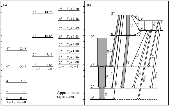
Figure 9: Level scheme for the approximate solution to the $\mathrm{X}(5)$ Hamiltonian. Excitation energies of the lowest members of the ground, $\beta$, and $\gamma$ bands, normalized to $E(2^{+}_{1})$, are shown at left. Electric quadrupole transition strengths, normalized to $B(E2;2^{+}_{1}\rightarrow 0^{+}_{1})=100$, are shown at right. The $\gamma$ band head energy $E_{\gamma}$ in part (a) and the $\gamma$ band transition strength normalizations $x$ and $y$ in part (b) depend upon the details of the $\gamma$ potential and are thus left unspecified. For plotting purposes, the $\gamma$ band head position and arrow thickness scales have been arbitrarily chosen to facilitate comparison with Fig. 2 (top). All observables involving the $\gamma$ band are calculated according to the approximate separation as it appears in Ref. iachello2001:x5 rather than in Ref. bijker2003:x5-gamma, which would yield values differing in detail endnote-bijkersep.

Since extensive prior work has been carried out using the approximate separation of variables of Ref. iachello2001:x5, it is useful to review this approximation, compare the results obtained under this separation with the exact results, and establish more clearly the reasons for the breakdown of the approximation. Two simplifications are required to obtain an approximate separation of variables for the Hamiltonian (1). First, in the limit of small $\gamma$, the sum $\sum_{\kappa}\hat{L}_{\kappa}^{\prime 2}/\sin^{2}(\gamma-2\pi\kappa/3)$ reduces to $4L(L+1)/3+K^{2}(1/\sin^{2}\gamma-4/3)$, where $L$ is the total angular momentum quantum number and $K$ the intrinsic frame angular momentum projection quantum number. Second, in all terms involving $\gamma$, the variable $\beta$ is replaced with a constant “average” value $\beta_{0}$. This yields a Hamiltonian $H=H_{\beta}+H_{\gamma}$ separable in the variables $\beta$ and $\gamma$,

$$H=\underbrace{-\frac{1}{\beta^{4}}\frac{\partial}{\partial\beta}\beta^{4}\frac{\partial}{\partial\beta}+\frac{L(L+1)}{3\beta^{2}}+V_{\beta}(\beta)}_{H_{\beta}}\,+\,\underbrace{{\frac{1}{\beta_{0}^{2}}\left[-\frac{1}{\sin 3\gamma}\frac{\partial}{\partial\gamma}\sin 3\gamma\frac{\partial}{\partial\gamma}+\frac{K^{2}}{4}\left(\frac{1}{\sin^{2}\gamma}-\frac{4}{3}\right)\right]+V_{\gamma}(\gamma)}}_{H_{\gamma}}.$$ (3)

The eigenvalues and eigenfunctions of $H_{\beta}$ are given by $\varepsilon_{\beta}=x^{2}_{\nu,s}$ ($s=0,1,\ldots$) and $f(\beta)\propto\beta^{-3/2}J_{\nu}(\varepsilon_{\beta}^{1/2}\beta)$ ($0\leq\beta\leq 1$), where $\nu=[L(L+1)/3+9/4]^{1/2}$ and $x_{\nu,s}$ is the $s$th zero of $J_{\nu}$ iachello2001:x5. Under the small $\gamma$ approximation, the eigenproblem for $H_{\gamma}$ reduces to that of the two-dimensional isotropic oscillator, with quantum numbers $n_{\gamma}$ and $K$, and the eigenvalues $\varepsilon_{\gamma}$ and eigenfunctions $\eta(\gamma)$ are as described in Ref. iachello2001:x5. The full eigenfunctions of $H$ are products $f_{Ls}(\beta)\eta_{n_{\gamma}K}(\gamma)\phi^{L}_{MK}(\vartheta)$ of a $\beta$ (“radial”) wave function, a $\gamma$ wave function, and a rotational or Euler angle ($\vartheta$) wave function $\phi^{L}_{MK}(\vartheta)$, defined in terms of $D$ functions as in Sec. II.

Under these approximations, the $\mathrm{X}(5)$ model yields levels arranged in bands of good $K$ quantum number, but with level energies [Fig. 9(a)] and $E2$ transition strengths [Fig. 9(b)] which differ from those of the rigid rotor. All predictions for the ground state band and $\beta$ excitations are independent of $V_{\gamma}$. The spin dependence of level energies within the yrast band is intermediate between those of the rigid rotor and harmonic oscillator, with $R_{4/2}\equiv E(4^{+}_{1})/E(2^{+}_{1})\approx 2.90$. The band arising from the first $\beta$ excitation occurs at low energy [$E(0^{+}_{\beta})/E(2^{+}_{1})\approx 5.65$].

Some of the characteristic spectroscopic features found in the approximate solution (discussed in detail in, e.g., Refs. iachello2001:x5; caprio2002:156dy-beta; bijker2003:x5-gamma) are indeed encountered in the full solution (Sec. III). The $\beta$ band exhibits a substantially larger energy spacing scale than the yrast band [$E(2^{+}_{\beta})-E(0^{+}_{\beta})\approx(1.80)E(2^{+}_{1})$]. Strong interband $E2$ transitions are predicted, as is the distinctive branching pattern in which the spin-descending $\beta$ to ground band transitions are suppressed.

However, some of the essential features of the full solution are missing from the approximate solution: the dependence of the $\beta$ band head energy upon $\gamma$ stiffness, the confinement of the wave functions near $\beta=1$ due to the five-dimensional centrifugal effect, and the consequent tendency of energy and transition strength observables towards rotational values for large $\gamma$ stiffness. Also, the observable signatures of $\gamma$-softness obtained in the full solution for realistic $\gamma$ stiffnesses, such as the staggering of energies in the $\gamma$ band, are absent under the approximate separation of variables, which effectively enforces $\gamma$ rigidity in the separation process.

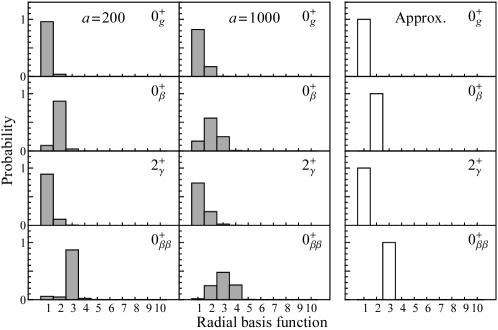
Figure 10: Probability decompositions of the true $\mathrm{X}(5)$ wave functions with respect to the radial functions from the approximate solution, integrated over angular coordinates. Decompositions are shown for the ground, $\beta$, $\gamma$, and $\beta\beta$ band heads, for $a=200$ (left) and $a=1000$ (middle). The relevant radial wave function under the approximate separation is indicated (right) for comparison. A basis of $L=0$ radial wave functions from the approximate solution ($\nu=3/2$) has been used for decomposition of the $0^{+}$ states, while a basis of $L=2$ radial wave functions ($\nu=\sqrt{7}/2$) has been used for decomposition of the $2^{+}_{\gamma}$ state.

The basic reason for the failure of the approximate solution to reproduce these features is clear from the analysis of Sec. III. The approximate Hamiltonian (3) retains only a portion of the centrifugal ($1/\beta^{2}$) contribution to the full Hamiltonian (1). Through the term $L(L+1)/(3\beta^{2})$, the portion of the centrifugal effect arising from rotational kinetic energy is essentially retained. But the replacement of $1/\beta^{2}$ by $1/\beta_{0}^{2}$ in the remaining terms suppresses the portion of the centrifugal effect arising from the $\gamma$ kinetic energy.

For a more detailed understanding of the breakdown of the approximate separation, we can reexamine the two approximations made in obtaining Eqn. (3).

(1) The small angle approximation for $\gamma$ is in principle arbitrarily good for sufficiently large $\gamma$ stiffnesses. However, as discussed in Sec. III [Fig. 4 (right)], confinement to genuinely small angles requires relatively large $\gamma$ stiffnesses ($a\gtrsim 1000$).

(2) The validity of the other approximation, replacement of $\beta$ with $\beta_{0}$ in selected terms, depends upon one of two conditions being met. The approximation would be good if the wave function were sharply localized in $\beta$, so indeed $\beta\approx\beta_{0}$. This condition may hold in some other contexts, such as small oscillations for a rigid rotor bohr1998:v2, but it is not well satisfied for the $\mathrm{X}(5)$ problem, which was specifically constructed to give a lack of $\beta$ localization. Even without reference to the exact solution, it is seen from the approximate radial wave functions $f_{sL}(\beta)$ that the the probability distribution with respect to $\beta$ is broad and differs significantly from state to state. For the approximate ground state $\langle 0^{+}_{1}|\beta^{-2}|0^{+}_{1}\rangle\approx 3.90$, while for the $\beta$ band head $\langle 0^{+}_{\beta}|\beta^{-2}|0^{+}_{\beta}\rangle\approx 7.21$, nearly a factor of two larger. Thus, replacing $1/\beta^{2}$ by a “rigid” value $1/\beta_{0}^{2}$ is not necessarily a small approximation. Alternatively, the replacement of $\beta$ with $\beta_{0}$ could still yield accurate results if the overall strength of the approximated term were small. This is seen from Sec. III to occur when the kinetic energy in the $\gamma$ degreee of freedom is small, and hence for nearly $\gamma$-soft potentials.

The two approximations are thus valid at large $\gamma$ stiffness and small $\gamma$ stiffness, respectively. If these two regimes are to have any overlap, it must be at some intermediate $\gamma$ stiffness. Indeed, as noted above, there is considerable qualitative agreement between the exact spectrum for $a=200$ [Fig. 2 (top)] and the approximate spectrum [Fig. 9]. However, the significance of this resemblance should not be overstated, since more detailed calculations reveal that it arises in part from a cancellation of errors introduced by the two approximations. The small angle approximation tends to cause an overcalculation of the $\beta$ band head energy, while the rigid $\beta$ approximation tends to cause an undercalculation.

A probability decomposition of the true wave functions with respect to the approximate radial wave functions $f_{Ls}$, summed over angular wave functions, provides a direct measure of the resemblance of the true and approximate eigenstates. This decomposition is shown in Fig. 10 (left, center) for several states, for $a=200$ and $1000$. The relevant radial basis state from the approximate solution is also indicated, for comparison [Fig. 10 (right)]. For intermediate $\gamma$ stiffness, the approximate solution indeed dominates the decomposition of the true solution, e.g., with a $96\%$ probability for the $s=1$ basis state in the true $a=200$ ground state [Fig. 10 (left)]. The similarity in wave functions breaks down for larger $\gamma$ stiffness [Fig. 10 (center)].

In summary, the approximate separation of variables of Ref. iachello2001:x5 causes the contribution of the $\gamma$ kinetic energy to the five-dimensional centrifugal effect to be suppressed. This is always a significant contribution and is the dominant portion for large $\gamma$ stiffness. The approximate solution for the $\mathrm{X}(5)$ Hamiltonian qualitatively reproduces some aspects of $\beta$-soft transitional structure, but only those which are least strongly affected by the $\beta$-$\gamma$ interaction. The approximate results quantitatively resemble the exact results only for a small range of $\gamma$ stiffnesses, in the vicinity of $a=200$. This is approximately the $\gamma$ stiffness of phenomenological interest for description of the rare earth ($N\approx 90$) transitional region. Consequently, many of the basic conclusions found in prior comparisons with experimental data casten2001:152sm-x5; bizzeti2002:104mo-x5; kruecken2002:150nd-rdm; caprio2002:156dy-beta; dewald2002:150nd-rdm; caprio2003:diss; hutter2003:104mo106mo-rdm; clark2003:x5-search; tonev2004:154gd-rdm; mccutchan2004:162yb-beta; mccutchan2005:166hf-beta remain largely unaffected.

V Conclusion

The numerical techniques of Rowe et al. rowe2004:tractable-collective; rowe2004:spherical-harmonics; rowe2005:collective-algebraic provide a practicable approach to the exact diagonalization of the $\mathrm{X}(5)$ Hamiltonian. The wave functions and spectroscopic properties obtained thereby provide insight into the structural features expected for $\beta$-soft, axially stabilized transitional nuclei. The properties of the solution are found to be dominated by the $\beta$-$\gamma$ coupling induced by the kinetic energy operator, which results in a significant five-dimensional centrifugal effect. Most spectroscopic properties are strongly dependent upon the $\gamma$ stiffness. The results also highlight the presence of substantial dynamical $\gamma$ softness. These basic qualitative features were not apparent from the approximate solution. The analysis in the present work can readily be extended to Hamiltonians which provide a more realistic treatment of transitional nuclei.

Appendix A Matrix elements

In this appendix a summary is provided of the procedure for calculating the necessary matrix elements of operators between radial or angular basis functions. The matrices of operators in the full product basis are obtained as the outer products of the radial and angular matrices. The radial basis functions $f_{i}(\beta)$ are defined inside the well ($0\leq\beta\leq 1$) as $f_{i}(\beta)=A_{\nu,i}\beta^{-3/2}J_{\nu}(x_{\nu,i}\beta)$ and are vanishing outside the well, where $x_{\nu,i}$ is the $i$th zero of $J_{\nu}$ and $A_{\nu,i}=[-J_{\nu-1}(x_{\nu,i})J_{\nu+1}(x_{\nu,i})]^{-1/2}$. For fixed $\nu$ and for $i=1$, $2$, $\ldots$, these form an orthonormal set of functions with respect to the metric $\beta^{4}d\beta$. The angular basis functions are constructed as sums of the form $\Psi_{v\alpha{}LM}(\gamma,\vartheta)=\sum_{\begin{subarray}{c}K=0\\ \text{even}\end{subarray}}^{L}F_{v\alpha{}LK}(\gamma)\phi^{L}_{MK}(\vartheta)$ according to the procedure of Ref. rowe2004:tractable-collective. These are orthonormal with respect to the metric $\lvert\sin 3\gamma\rvert d\gamma d\vartheta$. The $\phi^{L}_{MK}$ are symmetrized combinations of $D$ functions, $\phi^{L}_{MK}(\vartheta)\equiv[(2L+1)/(16\pi^{2}(1+\delta_{K}))]^{1/2}[D^{L}_{MK}(\vartheta)+(-)^{L}D^{L}_{M-K}(\vartheta)]^{*}$, and are orthonormal under integration over the Euler angles, except that $\phi^{L}_{MK}=0$ in the special case of $K=0$ and $L$ odd.

Matrix elements of an arbitrary function $g(\beta)$ between radial basis functions are calculated by straightforward numerical integration, as

$$\langle f_{i^{\prime}}|g(\beta)|f_{i}\rangle=\int\beta^{4}d\beta f_{i^{\prime}}(\beta)g(\beta)f_{i}(\beta).$$ (4)

The matrix elements of the radial kinetic energy operator in Eqn. (1) can be reexpressed in terms of matrix elements of $\beta^{-2}$ by use of the Bessel equation, as

$$\langle f_{i^{\prime}}|\left(\frac{1}{\beta^{4}}\frac{\partial}{\partial\beta}\beta^{4}\frac{\partial}{\partial\beta}\right)|f_{i}\rangle\\ =x_{\nu,i}^{2}\delta_{i^{\prime}i}-\left(\nu^{2}-9/4\right)\langle f_{i^{\prime}}|\beta^{-2}|f_{i}\rangle.$$ (5)

Observe that for the $\mathrm{X}(5)$ Hamiltonian the matrix elements of $V_{\beta}$ vanish, since $V_{\beta}(\beta)=0$ inside the well. The presence of the square well radial potential thus enters the calculations only implicitly, through the boundary condition it places on the allowed basis functions, which in turn dictates their kinetic energy matrix elements (5).

The matrix elements of an arbitrary function $f(\gamma)$, such as the function $\gamma^{2}$ appearing in the angular potential, can be calculated through a series of straightforward integrations involving the coefficients $F_{v\alpha{}LK}(\gamma)$, as rowe2004:tractable-collective

$$\langle\Psi_{v^{\prime}\alpha^{\prime}L}\|f(\gamma)\|\Psi_{v\alpha L}\rangle=\langle\Psi_{v^{\prime}\alpha^{\prime}LL}|f(\gamma)|\Psi_{v\alpha LL}\rangle\\ =\sum_{\begin{subarray}{c}K\\ \text{even}\end{subarray}}\int\lvert\sin 3\gamma\rvert d\gamma F_{v^{\prime}\alpha^{\prime}LK}^{*}(\gamma)f(\gamma)F_{v\alpha LK}(\gamma).$$ (6)

Here the Wigner-Eckart normalization convention of Rose rose1957:am has been used in the definition of the reduced matrix element. The integration can be restricted to $0\leq\gamma\leq\pi/3$ by periodicity of the functions in $\gamma$ rowe2004:tractable-collective. The expression (6) is readily extended, by application of the Clebsch-Gordan series, to give the matrix element of any spherical tensor operator $f^{\lambda}_{\mu}(\gamma,\vartheta)$, provided it is expanded in terms of $D$ functions as $f^{\lambda}_{\mu}(\gamma,\vartheta)=\sum_{\begin{subarray}{c}\kappa=0\\ \text{even}\end{subarray}}^{\lambda}f^{\lambda}_{\kappa}(\gamma)\phi^{\lambda\,*}_{\mu\kappa}(\vartheta)$. The matrix element is

$$\langle\Psi_{v^{\prime}\alpha^{\prime}L^{\prime}}\|f^{\lambda}(\gamma,\vartheta)\|\Psi_{v\alpha L}\rangle=\frac{1}{4\pi}\left[\frac{(2L+1)(2\lambda+1)}{2L^{\prime}+1}\right]^{1/2}\sum_{\begin{subarray}{c}K^{\prime},\kappa,K\\ \text{even}\end{subarray}}\left[\frac{1+\delta_{K^{\prime}}}{(1+\delta_{K})(1+\delta_{\kappa})}\right]^{1/2}\\ \times\left[(LK\lambda\kappa|L^{\prime}K^{\prime})+\env@cases(-)^{\lambda}(LK\lambda\bar{\kappa}|L^{\prime}K^{\prime}&K\geq\kappa\\ (-)^{L}(L\bar{K}\lambda\kappa|L^{\prime}K^{\prime})&K\leq\kappa\right\}\right]\left[\int\lvert\sin 3\gamma\rvert d\gamma F_{v^{\prime}\alpha^{\prime}L^{\prime}K^{\prime}}^{*}(\gamma)f^{\lambda}_{\kappa}(\gamma)F_{v\alpha LK}(\gamma)\right].$$ (7)

FortheleadingorderE2transitionoperator

bohr1998:v2,M(E2;μ)∝β[D2∗μ0cosγ+12(D2∗μ2+D2∗μ-2)sinγ],theexpansioncoefficientsaref^2_0(γ)∝(8π^2/5)^1/2cosγandf^2_2(γ)∝(8π^2/5)^1/2sinγ.T