Vector-Isovector Excitations at Finite Density and Temperature and the Validity of Brown-Rho Scaling

Abstract

Recent work reported at the Quark Matter Conference 2005 has led to the suggestion that Brown-Rho scaling is ruled out by the NA60 data. (Brown-Rho scaling describes the reduction of hadronic masses in matter and at finite temperature.) In the present work we argue that the interpretation of the experimental data presented at the Quark Matter Conference is not correct and that Brown-Rho scaling is valid. To make this argument we discuss the evolution in time of the excited hadronic system and suggest that the system is deconfined at the earliest times and becomes confined when the density and temperature decrease as the system evolves. Thus, we suggest that we see both the properties of the deconfined and confined systems in the experimental data. In our interpretation, Brown-Rho scaling refers to the later times of the collision, when the system is in the confined phase.

I INTRODUCTION

There has been an ongoing attempt to understand how quantum chromodynamics, the theory of strong interactions, governs the properties of hadrons in vacuum and in matter. Associated with this program are investigations of the properties of the quark-gluon plasma and of hadronic matter at finite temperature and finite matter density. (Experimental data concerning mesons in matter are often discussed in terms of Brown-Rho (BR) scaling [1]. Recent reviews may be found in Refs. [2,3].)

Various authors have discussed the behavior of meson masses in matter. For example, Hatsuda and Lee obtain

$$m_{\rho}^{*}=m_{\rho}(1-0.18\,n_{B}/n_{0}),$$ (1.1)

using QCD sum rules [4]. Here $n_{B}$ is the baryon density and $n_{0}$ is the density of nuclear matter. The Brooklyn College Group has also studied the properties of mesons at finite temperature and finite density [5-12] and we will make use of their results as we proceed.

The experimental data [13] obtained by the NA60 experiment is shown in Fig. 1 [14]. There the solid curve corresponds

$$m_{\rho}^{*}=m_{\rho}(1-0.15\,n_{B}/n_{0}),$$ (1.2)

while the dashed curve represents

$$m_{\rho}^{*}=m_{\rho}(1-0.15\,n_{B}/n_{0})\,\,(1-[T/T_{c}]^{2})^{0.3}.$$ (1.3)

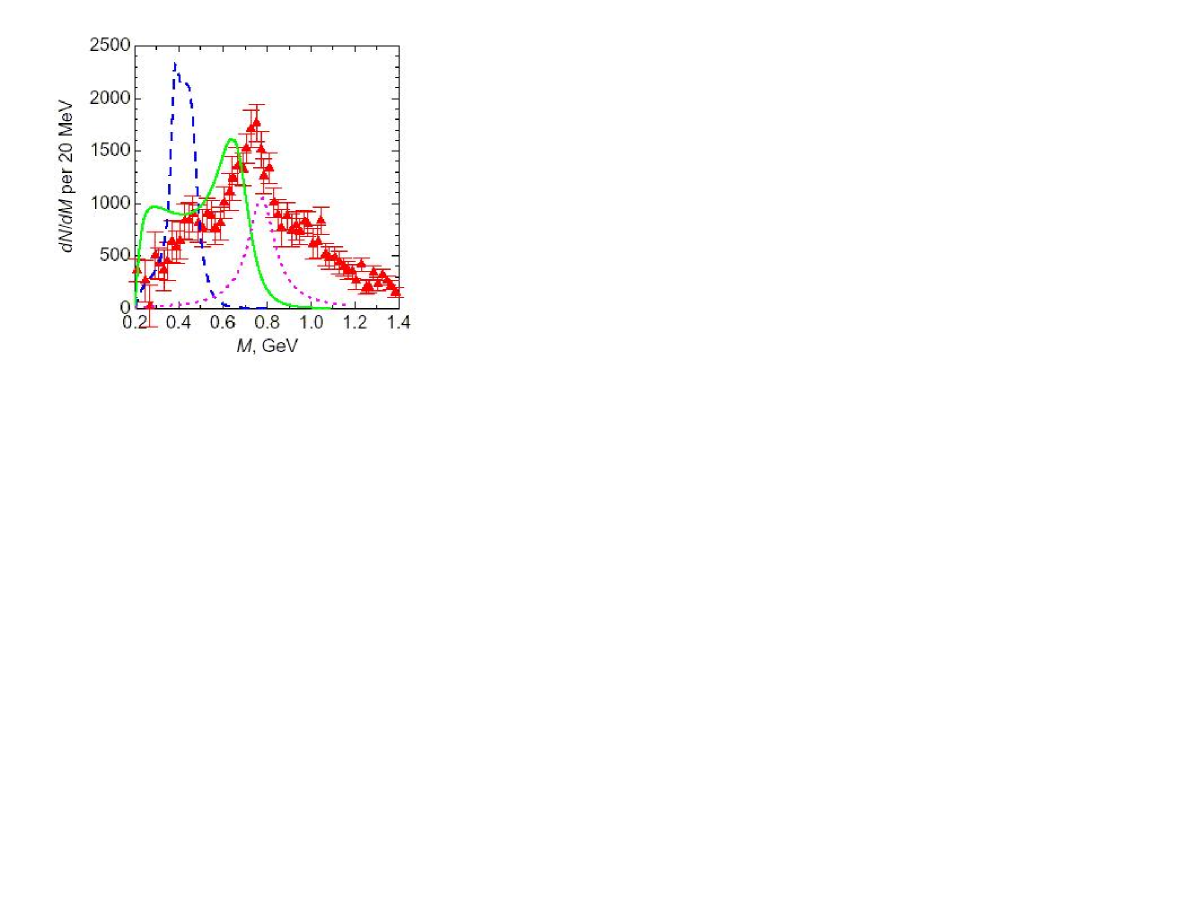
Figure 1: Invariant mass distribution of dimuons from semi-central In+In collisions at the beam energy $158$A GeV. Experimental points are from [13]. The solid and dashed curves are calculated using the $\rho$-mass modification factors of Eqs. (1.2) and (1.3), respectively. The dotted line indicates the hydrodynamically calculated $\rho$-meson decay at the freeze-out. (This figure appears in Ref. [14].)

The dilepton rate is given in Ref. [14] as

$$\frac{d^{8}N}{d^{4}xd^{4}q}=-\mathcal{L}(M)\,\,\frac{\alpha^{2}}{\pi^{3}q^{2}}\,\,f_{B}(q_{0},1/T)\,\,\mbox{Im}\Pi_{em}(q,T,\mu_{b}),$$ (1.4)

where $q^{2}=M^{2}=q_{0}^{2}-\vec{q}\,\,^{2}$. The Bose distribution function is

$$f_{B}(q_{0},\beta=1/T)=(e^{\beta q_{0}}-1)^{-1},$$ (1.5)

and the lepton kinematic factor is

$$\mathcal{L}(M)=\left(1+\frac{2m_{l}^{2}}{M^{2}}\right)\,\,\sqrt{1-\frac{4m_{l}^{2}}{M^{2}}},$$ (1.6)

with lepton mass $m_{l}$. If the pole shift is neglected, the imaginary part of the current correlation function is [14]

$$\mbox{Im}\Pi_{em}(M)=\frac{m_{\rho}^{4}}{g^{2}}\,\,\frac{\mbox{Im}\Pi(M)}{(M^{2}-m_{\rho}^{2})^{2}+\mbox{Im}\Pi^{2}(M)},$$ (1.7)

with

$$\mbox{Im}\Pi(M)=-\frac{g^{2}_{\rho\pi\pi}}{48\pi}\,\,\frac{(M^{2}-4m^{2}_{\pi})^{3/2}}{M},$$ (1.8)

$$\approx-\frac{g^{2}_{\rho\pi\pi}}{48\pi}M^{2}.$$ (1.9)

In the present work we will present results for the hadronic correlation function obtained in earlier studies for values of $T>T_{c}$ and $T<T_{c}$ [5-12].

In recent years we have developed a generalized Nambu-Jona-Lasinio (NJL) model that incorporates a covariant model of confinement. The Lagrangian of the model is

$${\cal L}= \bar{q}(i\hbox to0.0pt{\hbox to5.30904pt{\hfil/\hfil}\hss}\partial-m^{0})q+\frac{G_{S}}{2}\sum_{i=0}^{8}[(\bar{q}\lambda^{i}q)^{2}+(\bar{q}i\gamma_{5}\lambda^{i}q)^{2}]$$ (1.10)

$$-\frac{G_{V}}{2}\sum_{i=0}^{8}[(\bar{q}\lambda^{i}\gamma_{\mu}q)^{2}+(\bar{q}\lambda^{i}\gamma_{5}\gamma_{\mu}q)^{2}]$$

$$+\frac{G_{D}}{2}\{\det[\bar{q}(1+\gamma_{5})q]+\det[\bar{q}(1-\gamma_{5})q]\}$$

$$+{\cal L}_{conf}\,$$

where the $\lambda^{i}(i=0,\cdots,8)$ are the Gell-Mann matrices, with $\lambda^{0}=\sqrt{2/3}\mathbf{\,1}$, $m^{0}=\mbox{diag}\,(m_{u}^{0},m_{d}^{0},m_{s}^{0})$ is a matrix of current quark masses and ${\cal L}_{conf}$ denotes our model of confinement. Many applications have been made in the study of light meson spectra, decay constants, and mixing angles. In the present work we describe the use of our model when we include a description of deconfinement at finite density and temperature.

The organization of our work is as follows. In Section II we review results for mesonic excitations at finite matter density and at zero temperature. (It is of interest to note that the pion and kaon masses do not change very much with increasing density or temperature since these mesons are (pseudo) Goldstone bosons.) In Section III we discuss the properties of mesons at finite temperature in the confined mode. In Section IV we consider temperatures above $T_{c}$, the temperature for deconfinement. Above $T_{c}$, one finds resonant structures in the plasma which correspond to some of the excitations seen in computer simulations of QCD [15-22] whose analysis makes use of the maximum entropy method (MEM). Such excitations are also seen in our calculations made at finite density and zero temperature and are described in Section V.

In Section VI we return to a discussion of the NA60 data of Fig. 1 and argue that Brown-Rho scaling is indeed correct and that the experimental data supports our observation that the compound system evolves from the deconfined to the confined mode as the collision develops in time. Section VII contains some further comments and conclusions. Finally, in the Appendices, we review our model of confinement at finite temperature and at finite density.

II Mesonic Excitations at Finite Density

Figure 2: The density-dependent constituent quark masses, $m_{u}(\rho)=m_{d}(\rho)$ and $m_{s}(\rho)$ are shown. (See Ref. [12] and caption to Fig. 3.).

Figure 3: The dashed line is a linear approximation to the result shown in Fig. 2 which we use for $\rho\leq 2\rho_{NM}$. (Nuclear matter density corresponds to $k_{F}^{3}=0.0192$ GeV³.) See Ref. [12].

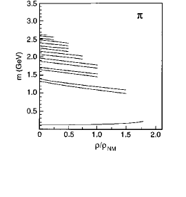
Figure 4: The mass values for the pion and its radial excitations are presented as a function of the density of matter. Here, the NJL model was used with density-dependent coupling constants, density-dependent masses and a density-dependent confining interaction [12]. [See the Appendices.] We use $G_{\pi}(\rho)=G_{\pi}(0)[1-0.087\rho/\rho_{NM}]$ and $m_{u}(\rho)=m_{d}(\rho)=m_{u}^{0}+0.3585\,\mbox{GeV}[1-0.4\rho/\rho_{NM}]$, with $m_{u}^{0}=0.0055$ GeV. We use $G_{\pi}(0)=13.49$ GeV^-2 and $G_{V}=11.46$ GeV^-2. Note that the various curves end at densities beyond which the excitations are no longer bound states.

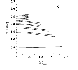
Figure 5: Mass values of the $K$ mesons are shown as a function of the density of matter. Here we use $G_{K}(0)=13.07$ GeV^-2, $G_{K}(\rho)=G_{K}(0)[1-0.087\rho/\rho_{NM}]$ and $G_{V}=11.46$ GeV^-2. (See Ref. [12].)

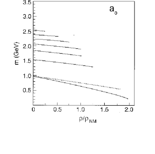
Figure 6: Mass values for the $a_{0}$ mesons are given as a function of the matter density. Here, we have used $G_{a_{0}}(0)=13.10$ GeV^-2 and $G_{a_{0}}(\rho)=G_{a_{0}}(0)[1-0.045\rho/\rho_{NM}]$. We have also used $m_{u}=m_{u}^{0}+0.3585\,\mbox{GeV}[1-0.4\rho/\rho_{NM}]$ with $m_{u}^{0}=0.0055$ GeV. The dotted line results if we put $G_{a_{0}}(\rho)=G_{a_{0}}(0)[1-0.087\rho/\rho_{NM}]$ and use the mass values of Table I of Ref. [12]. The dotted curve is similar to the curve for the $a_{0}$ mass given in Ref. [23]. The curves representing the masses of the radial excitations are changed very little when we use the second form for $G_{a_{0}}(\rho)$ given above. The dotted curve is reasonably well represented by $m^{*}_{a_{0}}(\rho)=m_{a_{0}}[1-0.22\rho/\rho_{NM}]$.

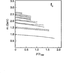
Figure 7: The figure shows the mass values of the $f_{0}$ mesons as a function of density. The mass values for the quarks are taken from Table I of Ref. [12]. In a singlet-octet representation, we have used the constants $G_{00}^{S}=14.25$ GeV^-2, $G_{08}^{S}=0.4953$ GeV^-2 and $G_{88}^{S}=10.65$ GeV^-2. Deconfinement takes place somewhat above $\rho=1.8\rho_{NM}$. (See Ref. [12].) For small $\rho/\rho_{NM}$, the mass of the $f_{0}$ is fairly well represented by $m^{*}_{f_{0}}(\rho)=m_{f_{0}}[1-0.14\rho/\rho_{NM}]$.

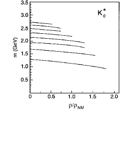
Figure 8: The figure shows the mass values obtained for the $K_{0}^{*}$ mesons as a function of density. Here we use a constant $G_{K_{0}^{*}}=10.25$ GeV^-2. Deconfinement takes place somewhat above $\rho=1.8\rho_{NM}$. For the smaller values of $\rho/\rho_{NM}$ the mass of the $K_{0}^{*}$ is given by $m^{*}_{K_{0}^{*}}(\rho)=m_{K_{0}^{*}}[1-0.14\rho/\rho_{NM}]$.

In this section we review some of the results reported in Ref. [5] for meson mass values at finite matter density. We made use of the density-dependent masses which are shown in Figs. 2 and 3. We also used density-dependent coupling constants in a generalized NJL model, in part to avoid pion condensation, and we have also introduced a density-dependent confining interaction [5]. Our model of confinement is discussed in Appendices A and B.

In Fig. 4 we see results for the pion and its various radial excitations. Note that the pion energy is fairly constant up to the point of deconfinement, since the pion is a (pseudo) Goldstone boson. In this case, deconfinement takes places at $\rho/\rho_{NM}\simeq 1.75$. In Fig. 5 we show corresponding results for the $K$ meson. Figs. 6 and 7 show our results for the $a_{0}$ and $f_{0}$ mesons, respectively. (The curve for the $f_{0}$ meson is reasonably well fit with $m_{f_{0}}^{*}=m_{f}(1-0.15\rho/\rho_{NM})$ for $\rho/\rho_{NM}<1.0$). Finally, in Fig. 8 we show our results for the $K_{0}^{*}$ meson mass as a function of density [12]. (In these calculations we have used the covariant confinement model which we review in the Appendices.)

The results presented in this Section are generally consistent with Brown-Rho scaling at finite density as represented by Eq. (1.1), for example. We see that our results are in agreement with those of Hatsuda and Lee [4], although we have used an entirely different method of calculation.

III Mesonic Excitations at Finite Temperature

Figure 9: The temperature-dependent constituent quark masses, $m_{u}(T)$ and $m_{s}(T)$, are shown. Here $m_{u}^{0}=0.0055$ GeV, $m_{s}^{0}=0.130$ GeV, and $G_{S}(T)=5.691[1-0.17(T/T_{c})]$, if we use Klevansky’s notation [24]. We have used the equation $m(T)=m^{0}+2G_{S}(T)N_{c}\frac{m(T)}{\pi^{2}}\int_{0}^{\Lambda}dp\frac{p^{2}}{E_{p}}\tanh(\frac{1}{2}\beta E_{p}),$ which appears in Ref. [24].

Calculations similar to those made at finite density have also been made at finite temperature [11]. In this case, temperature-dependent coupling constants were used in our generalized NJL model. The quark masses were calculated as a function of temperature and are shown in Fig. 9. Also, a temperature-dependent confining interaction was used based upon the lattice QCD analysis of Ref. [25]. (See Appendix B.)

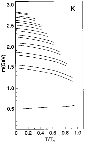
Figure 10: Mass values of kaonic states calculated with $G_{K}(T)=13.07[1-0.17\,T/T_{c}]$ GeV, $G_{V}(T)=11.46[1-0.17\,T/T_{c}]$ GeV, and the quark mass values given in Fig. 9. The value of the kaon mass is 0.598 GeV at $T/T_{c}=0.95$, where $m_{u}(T)=0.075$ GeV and $m_{s}(T)=0.439$ GeV. (See Ref. [11].)

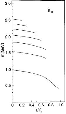
Figure 11: Mass values for the $a_{0}$ mesons calculated with $G_{a_{0}}(T)=13.1[1-0.17\,T/T_{c}]$ GeV, and the quark mass values given in Fig. 9. The value of the $a_{0}$ mass at $T/T_{c}=0.95$ is 0.416 GeV. (See Ref. [11].)

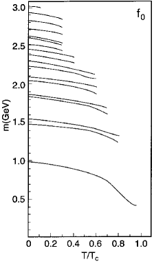
Figure 12: Mass values of the $f_{0}$ mesons calculated with $G_{00}(T)=14.25[1-0.17\,T/T_{c}]$ GeV, $G_{88}(T)=10.65[1-0.17\,T/T_{c}]$ GeV, $G_{08}(T)=0.495[1-0.17\,T/T_{c}]$ GeV, and $G_{80}(T)=G_{08}(T)$ in a singlet-octet representation. The quark mass values used are shown in Fig. 9. The $f_{0}$ has a mass of 0.400 GeV at $T/T_{c}=0.95$. (See Ref. [11].)

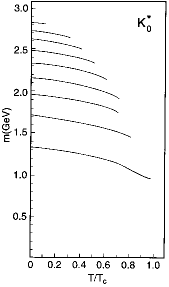
Figure 13: Mass values obtained for the $K_{0}^{*}$ mesons calculated using $G_{K_{0}^{*}}(T)=10.25[1-0.17\,T/T_{c}]$ GeV and the quark mass values shown in Fig. 9. (See Ref. [11].)

In Figs. 10-13 we show our results for the $K$, $a_{0}$, $f_{0}$ and $K_{0}^{*}$ mesons. In all these cases the mesons are no longer confined at energies slightly below $T_{c}$. (See Figs. 10-13.) In these calculations we find that the linear approximation $m^{*}(T)=m_{0}[1-\alpha T/T_{c}]$ is only satisfactory up to about $T/T_{c}\simeq 0.5$ for the $a_{0}$, $f_{0}$ and $K_{0}^{*}$ mesons.

IV Excitations of the Quark-Gluon Plasma at finite Density

For calculations at finite density we use the formalism of Ref. [8]. In this case the unusual form of the curves shown in Figs. 14 and 15 is due to Pauli blocking of the excitations by the filled states of the Fermi sea of quarks at finite density and zero temperature.

Figure 14: The figure presents values of the correlation function, $\mbox{Im}C_{\pi}(P^{2})$, for various values of $\rho/\rho_{c}$. Here, $\rho/\rho_{c}=1.2$ [solid line], 2.0 [dashed line], 3.0 [dotted line], 4.0 [dashed-dotted line] and 5.88 [dashed-(double)dotted line]. We have used $G_{\pi}=13.51$ GeV^-2. (See Ref. [8].)

Figure 15: The figure shown the values of $\mbox{Im}C_{\rho}(P^{2})$. [See the caption of Fig. 14.] Here we have used $G_{V}=11.46$ GeV^-2. (See Ref. [8].)

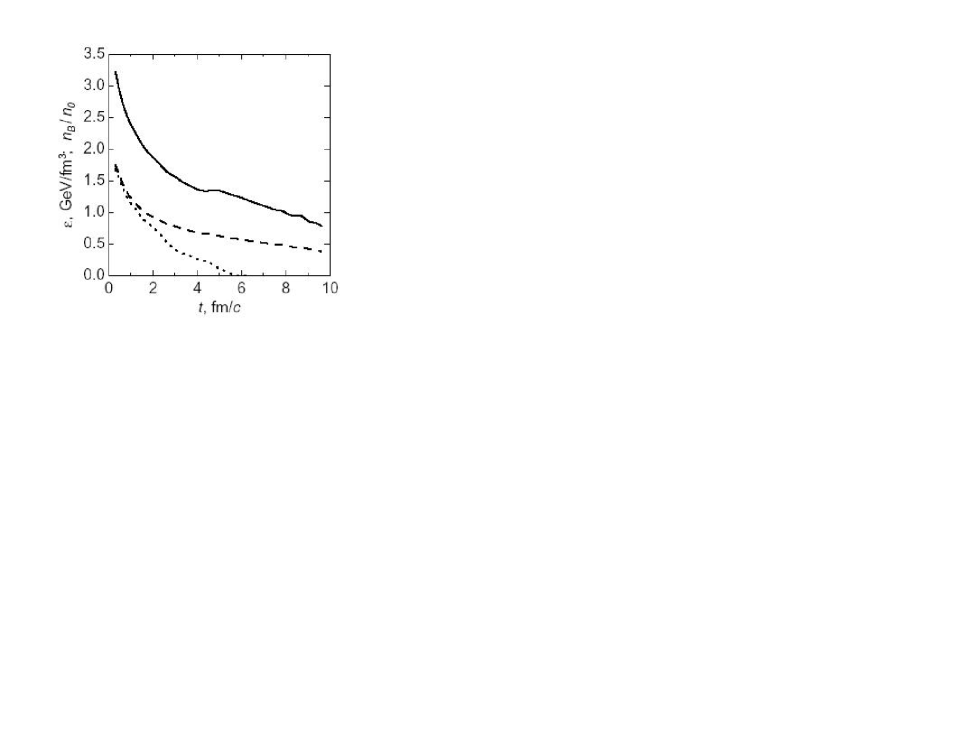
Figure 16: The average energy (solid line) and baryon (dashed) densities of an expanding fireball formed in In+In collisions. Dotted line shows a contribution of quarks and gluons to the energy density, as calculated in Ref. [14].

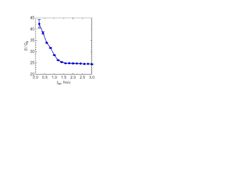
Figure 17: Temporal dependence of entropy $S$ per baryon charge $Q_{B}$ of participants for semi-central In+In collision at $E_{lab}=158A$ GeV, as calculated in Ref. [14].

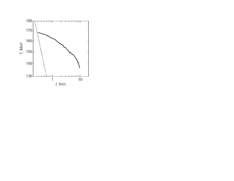
Figure 18: Evolution of the average temperature as calculated in Ref. [14]. The dotted line corresponds to the Bjorken regime with ultra-relativistic ideal gas EoS. (See Ref. [14].)

In Fig. 16, taken from Ref. [14], we show the calculated energy density and values of $n_{B}/n_{0}=\rho/\rho_{NM}$ relevant to the NA60 experiment. For times less than $t=1$ fm/c, $1.2\leq n_{B}/n_{0}\leq 1.7$.

In Fig. 17 the theoretical results for the ratio of the entropy $S$ to the baryon charge in the NA60 experiment is shown, as presented in Ref. [14] for the specific model used, the Quark-Gluon String Model. The authors of Ref. [14] suggest that for $t_{kin}\geq 1.3$ fm/c the system may be considered as undergoing isoentropic expansion.

In Fig. 18, taken from Ref. [14], the temperature is given as a function of $t_{kin}$. For $0<t_{kin}<1$ fm/c the temperature is in the range 162 MeV $\leq T\leq 170$ MeV. While these values are a bit below the deconfinement temperature at zero density, the value of $n_{B}/n_{0}$ is given as 1.7 at $t=0$. The combination of the elevated temperature and the finite matter density may be sufficient to keep the system in the deconfined phase at the earliest times of the collision, $t<1$ fm/c, as suggested in our analysis.

The authors of Ref. [14] suggest that the critical temperature (at the finite chemical potential $\mu_{B}$) is about 160 MeV. According to Fig. 18, taken from Ref. [14], the temperature drops below 160 MeV for $t\geq 1.3$ fm/c suggesting that the hadronic mode becomes dominant above that temperature. According to Fig. 16, the baryon density $n_{B}/n_{0}$ is approximately $1.0$ at $t\sim 1.3$ fm/c. Note that the dotted line in Fig. 16 represents the contribution of the quarks and gluons to the energy density in the model of Ref. [14].

V Excitations of the Quark-Gluon Plasma at finite Temperature

In this section we consider temperatures greater than $T_{c}$ and present the hadronic correlation functions calculated using the formalism of Ref. [7]. (We will not attempt to review that formalism here, but only present some our results.) For example, in Fig. 19 we show the correlation function in the vector-isovector channel. The position of the peaks may be moved by making small modifications of the coupling constant $G_{V}(T)$, whose temperature dependence is not well known. For the coupling constant that we have used for $T/T_{c}=1.2$, we find a peak in the spectral function at about 600 MeV. (Here the value used for $G_{V}$ is equal to 0.8 times the value of $G_{V}$ for $T=0$. See the Appendices for the definition of $G_{V}$.)

Figure 19: Values of $\mbox{Im}\,C_{V}(P_{0},T)/P_{0}^{2}$, obtained in Ref. [7], are shown for values of $T/T_{c}=1.2$ [ solid line ], $T/T_{c}=1.5$ [ dashed line ], $T/T_{c}=2.0$ [ dotted line ], $T/T_{c}=3.0$ [ dot-dashed line ], $T/T_{c}=4.0$ [ double dot-dashed line ], and $T/T_{c}=5.88$ [ short dashed line ]. Here we use $G_{V}(T)=G_{V}\,[1-0.17\,(T/T_{c})]$ with $T_{c}=0.150$ GeV and $G_{V}=11.46\,\mbox{GeV}^{-2}$.

VI discussion

We may return to a consideration of Fig. 1. We have suggested that the large peak at about 750 MeV represents the observation of the “prompt” leptons which are emitted for $t\leq 1$ fm/c when the system is in a deconfined mode. (We have argued that the elevated temperature and density is sufficient to deconfine the system at the earliest stage of the collision.) As the system moves into the confined phase for $t\geq 1$ fm/c we see that the curve for $S/Q_{B}$, seen in Fig. 17, changes its character, becoming constant for $t>1.5$ fm/c. That is suggestive of the formation of a confined phase in which we may discuss the validity of Brown-Rho scaling. (We remark that the peaks seen in Figs. 14, 15 and 16 do not represent bound-state mesons. Such mesons are deconfined at the elevated temperature and densities.)

We suggest that in the confined phase, the system generates the secondary peak seen in Fig. 1 at about 0.4-0.5 GeV. That is roughly in accord with the dashed curve representing Eq. (1.3). We also may suggest that the dashed curve peaks at a somewhat too low an energy since Eq. (1.3) leads to $m_{\rho}^{*}=0$ at $T=T_{c}$ which we believe overemphasizes the effect of temperature. (See Figs. 11-13 of Section III.)

If the interpretation of the NA60 data given in this work is correct, we may argue that the measurement of lepton pairs from vector-isovector states (resonances or bound states) can give us a detailed picture of the evolution of the deconfined system to the confined mode.

Recent work by Ruppert, Renk and M$\ddot{\mbox{{u}}}$ller contains a discussion of the width of the rho meson in a nuclear medium using QCD sum rules [26]. They are particularly concerned with how the width of the rho mass in the medium will affect the Brown-Rho scaling law

$$m_{\rho}^{*}/m_{\rho}\sim(<\bar{q}q>^{*}/<\bar{q}q>)^{1/2},$$ (6.1)

which is the more recent form of the scaling law [27,28] than that given in Ref. [1].

The widths of the rho in matter were calculated and presented in Fig. 2 of Ref. [26]. For the parameter set corresponding to the work of Hatsuda and Lee, the predicted width is approximately 300 MeV at $\rho/\rho_{NM}=1.5$. That is close to the width we may read from Fig. 1, when we consider the first peak in that figure at about 450-500 MeV. Therefore, our interpretation of the data is not incompatible with the analysis of Ref. [26]. Additional studies of the rho meson in matter may be found in Ref. [29]. Finally, we note that Brown and Rho have recently discussed the NA60 data and the validity BR scaling in Refs. [30, 31].

A recent experiment which describes the in-medium modification of the $\omega$ meson [37] provides support for BR scaling and the argument put forth in the present work. Reference [37] reports upon the photoproduction of the $\omega$ mesons on nuclei. They result for the $\omega$ mass in matter may be put into the form $m_{\omega}^{*}=m_{\omega}(1-0.14\rho/\rho_{0})$ where $\rho_{0}$ is the density of nuclear matter in the notation of Ref. [37]. We remark that since the experiment does not involve the creation of high temperature matter and a quark-gluon plasma, one does not expect to see the large peak seen in Fig. 1 which we have ascribed to excitations of the quark-gluon plasma with the quantum numbers of the rho meson.

Appendix A A model of confinement

There are several models of confinement in use. One approach is particularly suited to Euclidean-space calculations of hadron properties. In that case one constructs a model of the quark propagator by solving the Schwinger-Dyson equation. By appropriate choice of the interaction one can construct a propagator that has no on-mass-shell poles when the propagator is continued into Minkowski space. Such calculations have recently been reviewed by Roberts and Schmidt [32]. In the past, we have performed calculations of the quark and gluon propagators in Euclidean space and in Minkowski space. These calculations give rise to propagators which did not have on-mass-shell poles [33-36]. However, for our studies of meson spectra, which included a description of radial excitations, we found it useful to work in Minkowski space.

The construction of our covariant confinement model has been described in a number of works. In all our work we have made use of Lorentz-vector confinement, so that the Lagrangian of our model exhibits chiral symmetry. We begin with the form $V^{C}(r)=\kappa r\mbox{exp}[-\mu r]$ and obtain the momentum-space potential via Fourier transformation. Thus,

$$V^{C}(\vec{k}-\vec{k}\,^{\prime})=-8\pi\kappa\left[\frac{1}{[(\vec{k}-\vec{k}\,^{\prime})^{2}+\mu^{2}]^{2}}-\frac{4\mu^{2}}{[(\vec{k}-\vec{k}\,^{\prime})^{2}+\mu^{2}]^{3}}\right]\,,$$ (A1)

with the matrix form

$$\overline{V}\,{}^{C}(\vec{k}-\vec{k}\,^{\prime})=\gamma^{\mu}(1)V^{C}(\vec{k}-\vec{k}\,^{\prime})\gamma_{\mu}(2)\,,$$ (A2)

appropriate to Lorentz-vector confinement. The potential of Eq. (A1) is used in the meson rest frame. We may write a covariant version of $V^{C}(\vec{k}-\vec{k}^{\prime})$ by introducing the four-vectors

$$\hat{k}^{\mu}=k^{\mu}-\frac{(k\cdot P)P^{\mu}}{P^{2}}\,,$$ (A3)

and

$$\hat{k}^{\prime\,\mu}=k^{\prime\,\mu}-\frac{(k^{\prime}\cdot P)P^{\mu}}{P^{2}}\,.$$ (A4)

Thus, we have

$$V^{C}(\hat{k}-\hat{k}\,^{\prime})=-8\pi\kappa\left[\frac{1}{[-(\hat{k}-\hat{k}\,^{\prime})^{2}+\mu^{2}]^{2}}-\frac{4\mu^{2}}{[-(\hat{k}-\hat{k}\,^{\prime})^{2}+\mu^{2}]^{3}}\right]\,.$$ (A5)

Originally, the parameter $\mu=0.010$ GeV was introduced to simplify our momentum-space calculations. However, in the light of the following discussion, we can remark that $\mu$ may be interpreted as describing screening effects as they affect the confining potential [25]. In our work, we found that the use of $\kappa=0.055$ GeV² gave very good results for meson spectra.

The potential $V^{C}(r)=\kappa r\mbox{exp}[-\mu r]$ has a maximum at $r=1/\mu$, at which point the value is $V_{max}=\kappa/\mu e=2.023$ GeV. If we consider pseudoscalar mesons, which have $L=0$, the continuum of the model starts at $E_{cont}=m_{1}+m_{2}+V_{max}$, so that for $m_{1}=m_{2}=m_{u}=m_{d}=0.364$ GeV, $E_{cont}=2.751$ GeV. It is also worth noting that the potential goes to zero for very large r. Thus, there are scattering states whose lowest energy would be $m_{1}+m_{2}$. However, barrier penetration plays no role in our work. The bound states in the interior of the potential do not communicate with these scattering states to any significant degree. It is not difficult to construct a computer program that picks out the bound states from all the states found upon diagonalizing the random-phase-approximation Hamiltonian.

Appendix B density and temperature dependence of the confining field

In part, our study of the confining interaction has been stimulated by the results presented in Ref. [25] for the temperature-dependent potential, $V(r)$, in the case dynamical quarks are present. We reproduce some of the results of that work in Fig. 20. There, the filled symbols represent the results for $T/T_{c}=0.68,0.80,0.88$ and 0.94 when dynamical quarks are present. This figure represents definite evidence of “string breaking”, since the force between the quarks appears to approach zero for $r>1$ fm. This is not evidence for deconfinement, which is found for $T=T_{c}$. Rather, it represents the creation of a second $\bar{q}q$ pair, so that one has two mesons after string breaking. Some clear evidence for string breaking at zero temperature and finite density is reported in Ref. [25].

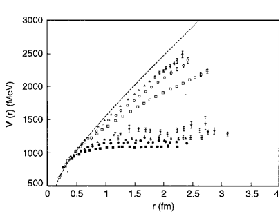
Figure 20: A comparison of quenched (open symbols) and unquenched results (filled symbols) for the interquark potential at finite temperature [25]. The dotted line is the zero temperature quenched potential. Here, the symbols for $T=0.80T_{c}$ [open triangle], $T=0.88T_{c}$ [open circle], $T=0.80T_{c}$ [open square], represent the quenched results. The results with dynamical fermions are given at $T=0.68T_{c}$ [solid downward-pointing triangle], $T=0.80T_{c}$ [solid upward-pointing triangle], $T=0.88T_{c}$ [solid circle], and $T=0.94T_{c}$ [solid square].

In order to study deconfinement in our generalized NJL model, we need to specify the interquark potential at finite density. In that case we had used $V^{C}(r)=\kappa r\mbox{exp}[-\mu r]$ for zero matter density. For the model we study in this work, we write

$$V^{C}(r,\rho)=\kappa r\mbox{exp}[-\mu(\rho)r]$$ (B1)

and put

$$\mu(\rho)=\frac{\mu_{0}}{1-\left(\displaystyle\frac{\rho}{\rho_{C}}\right)^{2}}\,,$$ (B2)

with $\rho_{C}=2.25\rho_{NM}$ and $\mu_{0}=0.010$ GeV. With this modification our results for meson spectra in the vacuum are unchanged. Other forms than that given in Eqs. (B1) and (B2) may be used. However, in this work we limit our analysis to the model described by these equations. The corresponding potentials for our model of Lorentz-vector confinement are shown in Fig. 21 for several values of $\rho/\rho_{NM}$. In the case of finite temperature we make use of the potentials $V^{c}(r,T)$ shown in Fig. 22.

Figure 21: Values of $V(r,\rho)$ are shown, where $V(r,\rho)=\kappa r\exp[-\mu(\rho)r]$ and $\mu(\rho)=\mu_{0}/[1-(\rho/\rho_{C})^{2}]$. Here $\rho_{C}=2.25\rho_{NM}$ and $\mu_{0}=0.010$ GeV. The values of $\rho/\rho_{NM}$ are 0.0 [solid line], 0.50 [dotted line], 1.0 [dashed line], 1.50 [dashed-dotted line]. 1.75 [dashed-dotted-dotted line], 2.0 [short-dashed line], and 2.1 [small dotted line].

Figure 22: The potential $V^{C}(r,T)$ is shown for $T/T_{c}=0$ [solid line], $T/T_{c}=0.4$ [dotted line], $T/T_{c}=0.6$ [dashed line], $T/T_{c}=0.8$ [dashed-dotted line], $T/T_{c}=0.9$ [short dashes], $T/T_{c}=1.0$ [dashed-(double) dotted line]. Here, $V^{C}(r,T)=\kappa r\exp[-\mu(T)r]$, with $\mu(T)=0.01\mbox{GeV}/[1-0.7(T/T_{c})^{2}]$ and $\kappa=0.055$ GeV².

References

• (1) G.E. Brown and M. Rho, Phys. Rev. Lett. 66, 2720 (1991).
• (2) W. Cassing and E.L. Bratkovskaya, Phys. Rep. 308, 65 (1999).
• (3) R. Rapp and J. Wambach, Adv. Nucl. Phys. 25, 1 (2000).
• (4) T. Hatsuda and S.H. Lee, Phys, Rev. C46, R34 (1992).
• (5) H. Li, C.M. Shakin, and Q. Sun, hep-ph/0310254.
• (6) B. He, H. Li, C.M. Shakin, and Q. Sun, Phys. Rev. C67, 065203 (2003).
• (7) B. He, H. Li, C.M. Shakin, and Q. Sun, Phys. Rev. D67, 114012 (2003).
• (8) B. He, H. Li, C.M. Shakin, and Q. Sun, hep-ph/0211318.
• (9) B. He, H. Li, C.M. Shakin, and Q. Sun, Phys. Rev. D67, 014022 (2003).
• (10) H. Li and C.M. Shakin, hep-ph/0209258.
• (11) H. Li and C.M. Shakin, hep-ph/0209136.
• (12) H. Li and C.M. Shakin, Phys. Rev. D66, 074016 (2002).
• (13) S. Scomparin $et\,\,al.$ (NA60 Collaboration) Plenary Talk at QM 2005.
• (14) V.V. Skokov and V.D. Toneev, nucl-th/0509085.
• (15) F. Karsch, M.G. Mustafa, and M.H. Thoma, Phys. Rev. Lett. B 497, 249 (2001).
• (16) M. Asakawa, T. Hatsuda, and Y. Nakahara, hep-lat/0208059.
• (17) T. Yamazaki $et\,\,al$., Phys. Rev. D 65, 014501 (2002).
• (18) M. Asakawa, T. Hatsuda, and Y. Nakahara, Prog. Part. Nucl. Phys. 46, 459 (2001).
• (19) Y. Nakahara, M. Asakawa, and T. Hatsuda, Phys. Rev. D 60, 091503 (1999).
• (20) I. Wetzorke, F. Karsch, E. Laermann, P. Petreczky, and S. Stickan, Nucl. Phys. B (Proc. Suppl.) 106, 510 (2002).
• (21) F. Karsch, S. Datta, E. Laermann, P. Petreczky, S. Stickan, and I. Wetzorke, hep-ph/0209028.
• (22) F. Karsch, E. Laermann, P. Petreczky, S. Stickan, and I. Wetzorke, Phys. Lett. B 530, 147 (2002).
• (23) C.M. Shakin and H. Wang, Phys. Rev. D 63, 114007 (2001).
• (24) S.P. Klevansky, Rev. Mod. Phys. 64, 649 (1992).
• (25) C. Detar, O. Kaczmarek, F. Karsch, and E. Laermann, Phys. Rev. D 59, 031501 (1998).
• (26) J. Ruppert, T. Renk and B. Muller, hep-ph/0509134.
• (27) G.E. Brown amd M. Rho, Phys. Rept. 269, 333 (1996).
• (28) G.E. Brown amd M. Rho, Phys. Rept. 363, 85 (2002).
• (29) S. Leupold, W. Peters and U. Mosel, Nucl. Phys. A 628, 311 9(1998).
• (30) G.E. Brown amd M. Rho,nucl-th/0509001.
• (31) G.E. Brown amd M. Rho,nucl-th/0509002.
• (32) C.D. Roberts and S.M. Schmidt. Prog. Part. Nucl. Phys., 45, S1 (2000).
• (33) C. Shakin, Ann. Phys., (N.Y.) 192, 254 (1989).
• (34) L.S. Celenza, C.M. Shakin, H.W. Wang, and X.H. Yang, Intl. J. Mod. Phys. A4, 3807 (1989).
• (35) V.M. Bannur, L.S. Celenza, H.H. Chen, S.F. Gao, and C.M. Shakin, Intl. J. Mod. Phys. A5, 1479 (1990).
• (36) X. Li and C.M. Shakin, Phys. Rev. D70, 114011 (2004).
• (37) D. Trnka, $et\,\,al.$ (CBELSA/TAPS Collaboration), Phys. Rev. Lett. 94, 192303 (2005).