Hanbury-Brown-Twiss Interferometry with Identical Bosons in Relativistic Heavy Ion Collisions: Comparisons with Hadronic Scattering Models

Abstract

Identical boson Hanbury-Brown-Twiss interferometry as applied to relativistic heavy-ion collisions is reviewed. Emphasis is placed on the use of hadronic scattering models to interpret the physical significance of experimental results. Interferometric studies with center-of-mass energies from $<1$ GeV/nucleon up to 5500 GeV/nucleon are considered.

1 Introduction

1.1 Scope of this Review

In the present work the application of the Hanbury-Brown-Twiss interferometry (HBT) technique to relativistic heavy-ion collisions (RHI) is reviewed. The emphasis is placed on comparing identical boson HBT experiments ranging in $\sqrt{s}$ from less than 1 GeV/nucleon to 200 GeV/nucleon with hadronic scattering models to attempt to understand what has been learned from these studies over the last twenty-five years. Predictions from such a model are also given for future LHC Pb+Pb collisions at $5500$ GeV/nucleon. Since the literature has been quite rich in this field during this period, it has been necessary to be selective both in the experiments and models which are presented. Thus, while in no way attempting to be comprehensive, an attempt has been made to present results in this work which are at least representative of the major developments in the field. More comprehensive reviews of this field can be found in the literature.[1, 2]

The review is organized as follows: the remainder of Section 1 gives a brief discussion of the original work of Hanbury-Brown and Twiss in developing HBT followed by the motivation for applying HBT to RHI, Section 2 gives some practical information to help understand how HBT is applied to RHI, Section 3 describes the hadronic scattering models discussed in this paper and presents comparisons of these models with results from two-boson HBT experiments, and Section 4 gives a summary.

1.2 Origins of HBT: Hanbury-Brown and Twiss experiments

About fifty years ago, Hanbury-Brown and Twiss first suggested, and then proved in a table-top experiment, that photon pairs exhibit a second-order interference effect if detected simultaneously in two detectors.[3] They applied this technique, which we now call HBT when applied with any type of boson,[4] to the measurement of the angular diameter of stars using pairs of photomultiplier tubes to detect optical photons[5] and pairs of radiotelescope dishes to detect longer wavelength photons.[6] Their measurement of the optical angular diameter of the star Sirius located in the constellation Canis Major, serves as a good example of the HBT method.[5] A schematic layout which helps to demonstrate the principle of their method is shown in Figure 1. Sirius is shown emitting two photons with wavevectors $\mathbf{k}_{i}$ and $\mathbf{k}_{j}$ from points $\mathbf{x}_{i}$ and $\mathbf{x}_{j}$, respectively, which are detected in two photomultiplier tubes located at positions $\mathbf{a}_{1}$ and $\mathbf{a}_{2}$ on the Earth.

file=fighbt1.eps,width=10cm

Figure 1: Schematic diagram of the method used to measure the angular diameter of Sirius by Hanbury-Brown and Twiss in 1956.

Assuming that photons are emitted incoherently from the star at each position and the photons are emitted as plane waves and taking a time-independent picture, the wavefunction to detect in coincidence the two photons in the two detectors on Earth, $\Psi(\mathbf{k}_{i},\mathbf{k}_{j};\mathbf{x}_{i},\mathbf{x}_{j})$, is

$$\Psi(\mathbf{k}_{i},\mathbf{k}_{j};\mathbf{x}_{i},\mathbf{x}_{j})=b[\exp(i\mathbf{k}_{i}\cdot(\mathbf{a}_{1}-\mathbf{x}_{i}))\exp(i\mathbf{k}_{j}\cdot(\mathbf{a}_{2}-\mathbf{x}_{j}))$$

$$+\exp(i\mathbf{k}_{i}\cdot(\mathbf{a}_{2}-\mathbf{x}_{i}))\exp(i\mathbf{k}_{j}\cdot(\mathbf{a}_{1}-\mathbf{x}_{j}))]$$ (1)

where the second term arises due to the path ambiguity of detecting bosons (as shown in Figure 1), and where $b$ is a normalization constant. The probability to detect the two photons, $P_{ij}$, is just the square of $\Psi$, i.e. $\Psi^{*}\Psi$, and thus given by

$$P_{ij}(\Delta\mathbf{k},\mathbf{d})=b^{2}[1+\cos(\Delta\mathbf{k}\cdot\mathbf{d})]$$ (2)

where $\Delta\mathbf{k}=\mathbf{k}_{i}-\mathbf{k}_{j}$ and $\mathbf{d}=\mathbf{a}_{1}-\mathbf{a}_{2}$. The separation between the two detectors, $d$, is called the baseline. It is seen in Eq. (2) that a) the $cos$ term in $P_{ij}$ is a result of the path ambiguity term in Eq. (1.2), and b) $P_{ij}$ does not depend on the photon emission positions at the star but only on the differences between the wavevectors and the detector positions. One can write Eq. (2) in a more convenient form with the approximations $k_{i}\simeq k_{j}\equiv k$, $\Delta\mathbf{k}\cdot\mathbf{d}\simeq\mid\Delta\mathbf{k}\mid$, $\mid\Delta\mathbf{k}\mid\simeq\theta_{ij}k=2\pi\theta_{ij}/\lambda$, taking $b=1$, and defining the correlator, $C_{ij}(d)\equiv P_{ij}-1$, resulting in

$$C_{ij}(d)=\cos(2\pi\theta_{ij}d/\lambda)$$ (3)

where, as seen in Figure 1, $\theta_{ij}$ is the angular diameter seen on Earth between the points on the star $i$ and $j$ and $\lambda$ is the wavelength of the photons. $C_{ij}(d)$ is proportional to the coincidence signal produced in the photomultipliers for the photons coming from these two points on the star, but in practice, the signal measured in the electronics is the sum over all of the photon emission point pairs from the star. If $N$ is defined as the number of photon source points making up a star of brightness (intensity) $I$ and radius $r$, to get the detected signal from the entire star, $C(d)$, $C_{ij}$ is summed over all of the unique pairs of photon emission points

$$C(d)=\epsilon\sum^{N}_{i>j}C_{ij}(d)=\epsilon\sum^{N}_{i>j}\cos(2\pi\theta_{ij}d/\lambda)$$ (4)

where $\epsilon$ is a conversion factor to get the detector signal. If one looks at cases where the arguments of the $cos$ terms in Eq. (4) are small such that the $cos$ terms are not far from unity, e.g. for small baselines, Eq. (4) can approximately be expressed as

$$C(d)\simeq\epsilon\frac{N^{2}}{2}\cos(2\pi\theta_{1}d/\lambda)$$ (5)

where $\theta_{1}$ is the average of the $\theta_{ij}$.

One is now in the position to measure the average angular size of a star by measuring $C(d)$ as a function of $d$ and fitting these data with Eq. (5) to extract $\theta_{1}$. Figure 2 shows measurements of $C(d)$ for Sirius by Hanbury- Brown and Twiss. Also plotted are fits to the data using Eq. (5) (taking $\lambda=550$ nm) and a full calculation including integrations over the photon wavelength spectrum and photon source distribution and detection efficiency effects by Hanbury-Brown and Twiss.[5] As seen, $\theta_{1}$ extracted from the fit to the data by Eq. (5) agrees with the angular diameter extracted from the fit by the full calculation within a factor of two.

file=fighbt2.eps,width=10cm

Figure 2: Measurement of $C(d)/C(0)$ vs. d for Sirius by Hanbury-Brown and Twiss. Also shown are fits to the measurements using Equation 4 and a full calculation.

Another example of applying the HBT technique to measure angular size is for the binary star Alpha Centauri, located in the constellation Centauris seen in the southern hemisphere. A schematic diagram of the geometry of the measurement is shown in Figure 3. For the orientation of the two stars shown, there are two angular size scales that enter this measurement: the angular sizes of the individual stars (assumed to be identical), $\theta_{1}$, and the angular size between the two stars, $\theta_{2}$. What angular size will the HBT technique measure? To answer this question, calculate $C_{binary}(d)$ using Eq. (4) assuming that the binary star has the total number of photon source points $N$ distributed equally between the two stars and setting $\epsilon=1$ for simplicity, giving

$$C_{binary}(d)=2\sum^{N/2}_{i>j}\cos(2\pi\theta_{ij}d/\lambda)+\sum^{N/2}_{i(A),j(B)}\cos(2\pi\theta_{ij}d/\lambda)$$ (6)

where the first sum accounts for the two identical sums over the individual stars in the binary, and the second sum accounts for the sum over photon source pairs between the two stars, i.e. the index $i$ associated with star A and $j$ with the star B. One can now use the same approximation as before in going from Eq. (4) to Eq. (5), i.e. the argument of the cosine being small, to express the first sum in Eq. (6) in terms of $\theta_{1}$. This will not be the case for the second sum, since for Alpha Centauri the separation between the stars, $L$, is much larger than the radius of the individual stars, $r$ ($L\simeq 11$ A.U. and $r\sim$ solar radius), resulting in $\theta_{2}>>\theta_{1}$. Thus, the $cos$ terms in the second sum will oscillate wildly, resulting in that sum vanishing, and Eq. (6) becomes

$$C_{binary}(d)=\frac{N^{2}}{4}\cos(2\pi\theta_{1}d/\lambda).$$ (7)

Comparing Eq. (7) with Eq. (5), it is seen that the binary star gives half the detected HBT signal expected from a star with $N$ photon source points, and its angular size is characterized by the size of the individual stars making up the binary. When Hanbury-Brown and Twiss performed such a measurement on Alpha Centauri, this is indeed what they observed.[7]

file=fighbt3.eps,width=10cm

Figure 3: Schematic diagram of the geometry for the measurement of the angular size of the binary star, Alpha Centauri.

This example of the use of this technique on a binary star shows that the particular boson source distribution of the system measured has an important impact on how results from HBT are interpreted. It will be shown later that similar effects are seen when applying this technique to two-pion measurements of RHI.

2 Applying HBT to Relativistic Heavy-Ion Collisions

Relativistic heavy-ion collisions are similar to stars in that they emit bosons from a finite-sized region (i.e. the interaction region). They differ from stars in that 1) the bosons are predominantly pions, 2) other bosons such as kaons are emitted, 3) the size scale is much smaller ($\sim 10^{-15}$ m), and 4) the lifetime of the boson-emitting source is short ($\sim 10^{-23}$ s), introducing time as an important variable. Nevertheless, one could imagine applying HBT to RHI to directly measure the size, and perhaps the lifetime, of these collisions and thus get information on their space-time dynamics. The first measurement of the pion-emitting source using two-pion interferometry was carried out by G. Goldhaber, S. Goldhaber, W. Lee, and A. Pais in 1960 with $\sqrt{s}=2.1$ GeV proton+antiproton collisions from the Bevatron (they referred to this method as Bose-Einstein correlations and others have called this the GGLP effect).[8] In this section a qualitative derivation is given for two-pion Bose-Einstein/HBT interferometry and a few practical considerations for carrying out experimental RHI HBT studies are given.

2.1 Qualitative derivation of two-pion HBT in RHI

A qualitative derivation of two-pion HBT interferometry is given below. More formal derivations can be found in the literature.[9, 2] As will be seen, its derivation will closely parallel that given earlier for two-photon HBT. A schematic diagram of the geometry of a two-pion interferometric measurement is given in Figure 4. The interaction region in a RHI collision is shown emitting two pions from points $\mathbf{x}_{i}$ and $\mathbf{x}_{j}$, which are detected with wavevectors $\mathbf{k}_{i}$ and $\mathbf{k}_{j}$ in two “pion detectors” located at positions $\mathbf{a}_{1}$ and $\mathbf{a}_{2}$, respectively, in the experimental hall.

file=fighbt4.eps,width=10cm

Figure 4: Schematic diagram of a two-pion interferometric measurement in which the pions are produced in a RHI collision.

Assuming that pions are emitted incoherently from the interaction region at each position and the pions are emitted as plane waves and taking a time-independent picture, the wavefunction to detect in coincidence the two pions with these wavevectors in the two detectors, $\Psi(\mathbf{k}_{i},\mathbf{k}_{j};\mathbf{x}_{i},\mathbf{x}_{j})$, is

$$\Psi(\mathbf{k}_{i},\mathbf{k}_{j};\mathbf{x}_{i},\mathbf{x}_{j})=b[\exp(i\mathbf{k}_{i}\cdot(\mathbf{a}_{1}-\mathbf{x}_{i}))\exp(i\mathbf{k}_{j}\cdot(\mathbf{a}_{2}-\mathbf{x}_{j}))$$

$$+\exp(i\mathbf{k}_{i}\cdot(\mathbf{a}_{1}-\mathbf{x}_{j}))\exp(i\mathbf{k}_{j}\cdot(\mathbf{a}_{2}-\mathbf{x}_{i}))]$$ (8)

where the second term arises due to the path ambiguity of detecting bosons (as shown in Figure 4), and where $b$ is a normalization constant. This expression is similar to Eq. (1.2) above used for photon pairs from a star, but not identical. The difference is that indices are switched in the second term since we assume the pion wavevector (momentum) is now associated with a particular detector, rather than with an emission point as in the case of a photon from the star. The ambiguity in this case is in which emission point the pion originates from, not which detector records a photon. The probability to detect the two pions, $P_{ij}$, is just the square of $\Psi$, i.e. $\Psi^{*}\Psi$, and thus given by

$$P_{ij}(\Delta\mathbf{k},\mathbf{r})=b^{2}[1+\cos(\Delta\mathbf{k}\cdot\mathbf{r})]$$ (9)

where $\Delta\mathbf{k}=\mathbf{k}_{i}-\mathbf{k}_{j}$ and $\mathbf{r}=\mathbf{x}_{i}-\mathbf{x}_{j}$. The separation between the two emission points, $r$, is related to the size of the interaction region or “pion source.” It is seen in Eq. (9) that a) the $cos$ term in $P_{ij}$ is a result of the path ambiguity term in Eq. (2.1), and b) $P_{ij}$ does not depend on the detector positions but only on the differences between the pion momenta and the emission positions. Note that the time variable can also be introduced into this formalism by considering $\mathbf{k}$ and $\mathbf{x}$ as four vectors.

As in the discussion of HBT with stars in the last section, the interaction region can emit pions from an extended region of points in space which the detectors sum over. Defining the pion source distribution function as a continuous function of the position of a source point $\mathbf{x}$, $\rho(\mathbf{x})$, one can integrate the interaction region over all pairs of source points using Eq. (9),

$$C(\Delta\mathbf{k})=\int P_{ij}(\Delta\mathbf{k},\mathbf{r})\rho(\mathbf{x_{i}})\rho(\mathbf{x_{j}})d\mathbf{x_{i}}d\mathbf{x_{j}},$$ (10)

where $C(\Delta\mathbf{k})$ is called the correlation function. Assuming for simplicity that the pion source is distributed as a gaussian of width $R$, i.e. $\rho(r)\sim\exp(-r^{2}/2R^{2})$, and substituting into Eq.(10) the result is,

$$C(\Delta\mathbf{k})\sim 1+\exp[-(\Delta\mathbf{k})^{2}R^{2}].$$ (11)

Figure 5. shows a two-pion HBT measurement in central RHIC Au+Au collisions from the STAR experiment, which detects charged particles in a large-acceptance Time Projection Chamber immersed in a magnetic field.[10] The one-dimensional two-pion correlation function (extracted from the two-pion coincidence count rate, see later) evaluated in the invariant frame of the pion source is plotted versus $\Delta k$. Only the data points lower than $\hbar\Delta k<50$ MeV/c are plotted. A version of Eq. (9) assuming $\Delta\mathbf{k}\perp\mathbf{r}$ including an arbitrary parameter $\lambda$ is fitted to the data to extract $r$ and $\lambda$ (dashed line). A version of Eq. (11) with the same parameters is also fitted (solid line). As seen, the gaussian function fits the data better, but both functions give about the same fitted values of $r\sim 8$ fm and $\lambda\sim 0.5-0.6$.

file=fighbt5.eps,width=10cm

Figure 5: Two-pion HBT in RHIC Au+Au collisions from the STAR experiment with fits. Only points for $\hbar\Delta k<50$ MeV/c are plotted.

What is the interpretation of these results for $r$ and $\lambda$? Naively, one would expect the size of the Au nucleus, $1.2A^{1/3}\sim 7$ fm, to set the scale for the size of the pion emitting source in these collisions, and this is seen to be the case for $r$. For $\lambda$ one might expect this to be unity for the idealized derivation of Eq. (9), yet the value extracted in this case is significantly smaller. This is suggestive of the reduced HBT signal seen in binary stars discussed above, for which boson sources of distinctly different sizes are intermixed.

How to interpret the parameters from such fits to data in RHI HBT analyses will be an important theme for the rest of this paper. As will be shown, models of the interaction will be used as tools to interpret experimental HBT results.

2.2 Measuring the Correlation Function in experiments

As shown in Figure 4., in carrying out an experimental HBT study one measures the two-boson coincident count rate along with the one-boson count rates for reference. The experimental two-boson correlation function for bosons binned in momenta $\mathbf{k_{1}}$ and $\mathbf{k_{2}}$, $C(\mathbf{k_{1}},\mathbf{k_{2}})$, is constructed from the coincident countrate, $N_{2}(\mathbf{k_{1}},\mathbf{k_{2}})$ and one-boson countrate, $N_{1}(\mathbf{k})$, as

$$C(\mathbf{k_{1}},\mathbf{k_{2}})=\alpha(\mathbf{k_{1}},\mathbf{k_{2}})\frac{N_{2}(\mathbf{k_{1}},\mathbf{k_{2}})}{N_{1}(\mathbf{k_{1}})N_{1}(\mathbf{k_{2}})},$$ (12)

where $\alpha(\mathbf{k_{1}},\mathbf{k_{2}})$ is a correction factor for non-HBT effects which may be present in the experiment. Typically,the largest contributions to $\alpha(\mathbf{k_{1}},\mathbf{k_{2}})$ occur in the correction for the boson detection efficiency and in correcting for final-state boson-boson Coulomb repulsion.[1] It is usually convenient to express the six-dimensional $C(\mathbf{k_{1}},\mathbf{k_{2}})$ in terms of the four-vector momentum difference, $Q=|k_{1}-k_{2}|$ by summing Eq.(12) over momentum difference,

$$C(Q)=\sum_{\mathbf{k_{1}},\mathbf{k_{2}}(Q)}\alpha(\mathbf{k_{1}},\mathbf{k_{2}})\frac{N_{2}(\mathbf{k_{1}},\mathbf{k_{2}})}{N_{1}(\mathbf{k_{1}})N_{1}(\mathbf{k_{2}})}=\epsilon(Q)\frac{A(Q)}{B(Q)},$$ (13)

where $A(Q)$ represents the “real” coincident two-boson countrate, $B(Q)$ the “background” two-boson countrate composed of products of the one-boson countrates and $\epsilon(Q)$ the correction factor, all expressed in $Q$. [2] In practice, $B(Q)$ is the mixed event distribution, which is computed by taking single bosons from separate events.[1]

2.3 Parameterizing the Correlation Function: extracting boson source parameters

The experimental two-boson correlation function is formed using Eq.(13) and a gaussian model for the boson source distribution is normally fitted to it to extract radius parameters. A standard parameterization of C(Q) is obtained by assuming a gaussian space-time distribution of freeze-out points, $\rho(r,t)$, in terms of the variables $r_{Tside}$, which points in the direction of the sum of the two boson momenta in the transverse plane, $r_{Tout}$, which points perpendicular to $r_{Tside}$ in the transverse plane, the longitudinal variable along the beam direction, z, and time, t:

$$\rho(r,t)=F\exp(-\frac{{r_{Tside}}^{2}}{2{R^{\prime}_{Tside}}^{2}}-\frac{{r_{Tout}}^{2}}{2{R^{\prime}_{Tout}}^{2}}-\frac{z^{2}}{2{R^{\prime}_{Long}}^{2}}-\frac{t^{2}}{2\tau^{2}})$$ (14)

where $R^{\prime}_{Tside}$ is a transverse sideward radius parameter, $R^{\prime}_{Tout}$ is a transverse outward radius parameter, $R^{\prime}_{Long}$ is a longitudinal radius parameter, $\tau$ is a lifetime parameter, and F is a normalization constant.[11] From this distribution function the following parameterization of C(Q) can be obtained :[12]

$$C(Q_{Tside},Q_{Tout},Q_{Long})=$$ (15)

$$G[1+\lambda\exp(-Q_{Tside}^{2}R_{Tside}^{2}-Q_{Tout}^{2}R_{Tout}^{2}-Q_{Long}^{2}R_{Long}^{2})]$$

where Q has been broken up into the two transverse and one longitudinal components, G is a normalization constant, and $\lambda$ is the usual empirical parameter added to help in the fitting of Eq. (15) to the actual correlation function ($\lambda=1$ in the ideal case). The radius parameters in Eq. (15) are related to those in Eq.(14) in, for example, the LCMS frame (longitudinally comoving system in which the longitudinal boson pair momentum vanishes) as follows:

$$R_{Tside}^{2} = {R^{\prime}_{Tside}}^{2}$$

$$R_{Tout}^{2} = {R^{\prime}_{Tout}}^{2}+\beta_{T}^{2}\tau^{2}$$ (16)

$$R_{Long}^{2} = {R^{\prime}_{Long}}^{2}$$

where $\beta_{T}$ is the transverse velocity of the boson pair. In this parameterization as seen from Eq. (2.3) $R_{Tout}$ contains information about both the transverse size and the lifetime of the source. Note that Eq.(15) follows from Eq.(14) under the assumption of a geometrically static boson source. In a realistic heavy-ion collision the source will not be static and may have position-momentum correlations and other effects that could make the source parameters defined above depend on the boson pair momentum . In the present application, Eq. (15) is fitted to the experimental correlation function to extract the radius parameters $R_{Tside}$, $R_{Tout}$, and $R_{Long}$ and $\lambda$. Figure 6 shows experimental $\pi^{-}-\pi^{-}$ correlation functions with and without final-state Coulomb corrections included from the Relativistic Heavy Ion Collider (RHIC) STAR experiment[10] for $\sqrt{s}=130$ GeV/nucleon Au+Au collisions along with gaussian fits.

file=fighbt6.eps,width=10cm

Figure 6: $\pi^{-}-\pi^{-}$ HBT in RHIC Au+Au collisions from the STAR experiment with gaussian fits. The Coulomb-corrected data are shown as filled circles and the uncorrected data as open circles (from Ref.[10]).

3 Comparing hadronic scattering models with two-boson HBT experiments from RHI collisions

Relativistic heavy-ion collisions provide a means of creating matter in a hot and dense state which might shed light on the behavior of matter under these extreme conditions, such as the possibility of producing a phase transition to quark matter.[13] It is generally agreed that the most extreme conditions exist in the initial state of the heavy-ion collision, roughly defined as occurring just after the projectile and target nuclei pass through each other. Eventually the interaction region hadronizes into a large number of mesons and baryons (with non-hadronic particles such as photons, electrons, and muons also being produced) and then expands to its final state. During the expansion stage the hadrons strongly scatter with each other, this process being called rescattering. The final state of the collision can be thought of as the state for which rescattering ceases among all remaining (final) hadrons. It is often convenient to define the “freezeout” point of a final hadron as the position, time, energy, and momentum the particle had when it stopped rescattering. Thus, one can define more precisely the final state of the collision as the collection of the freezeout points of all of the final hadrons in an 8-dimensional phase space (4 dimensions for space-time and 4 dimensions for momentum-energy). The term freezeout will be used to represent the final state of the collision defined in this way. In principle, the properties of the collision at freezeout are directly accessible by measurement. In practice, one directly measures the freezeout momenta and energies of the particles using, for example, magnetic spectrometers [11] and indirectly measures the freezeout space-time from the freezeout momenta and energies using the method of two-boson HBT interferometry.

However, the main motivation to study relativistic heavy-ion collisions is to obtain information about the initial, extreme state of the collision. Some directly measurable non- hadronic probes such as direct photons, and electron and muon pairs have been predicted to be sensitive to certain features of the initial state.[14] It is equally important to study the final hadrons from the collision since they should contain information about the bulk properties of the initial state, i.e. the temperature and energy density achieved in the collision. The difficulty in using the hadrons to extract this information is that the rescattering process masks the initial space-time and momentum-energy information by random scattering and thus there is no simple connection between the freezeout information obtained in experiments and the initial state.

In this paper, the method employed to approach this problem is to use hadronic scattering calculations to disentangle the rescattering effects from the hadronization process. The strategy will be to take a simple model for hadronization and propagate the initial hadrons via rescattering to freezeout, adjusting the parameters of this model to see if a parameter set can be found where the freezeout observables from the calculation agree with those measured in experiments. Within the context of such a model, this parameter set thus describes the state of the collision before rescattering, putting one a step closer in time to the initial state. The advantage of using a simple hadronization model is that the number of parameters to be adjusted is minimized, increasing the chances that the extracted parameter set is unique. The disadvantage is that some physics of the hadronization will be left out, so the physical interpretation of these parameters may be complicated. Descriptions of two such hadronic scattering models are presented below. Results of these models are then compared with RHI HBT experiments.

3.1 Intranuclear Cascade Model for $\sqrt{s}<$ 1 GeV/nucleon: INCM

Intranuclear cascade models (INCM) have been used extensively to understand general features of RHI collisions for bombarding energies of $\sqrt{s}<$ 1 GeV/nucleon.[15] The basic assumption in these models is that a RHI collision can be viewed as a superposition of nucleon-nucleon interactions whose trajectories between interactions are described classically while the interactions are determined by experimental scattering cross sections. The CASCADE code by Cugnon[16] is a version of a INCM. In this version, $\Delta$ isobars are included which serve as the mechanism through which pions are produced and rescattered throughout the duration of the collision. The CASCADE code is isospin averaged such that there is only one type of pion, nucleon, and $\Delta$ in the calculation. A pion is defined as freezing out from the calculation when it no longer scatters and the time and position of its parent $\Delta$, along with the vector momentum of the pion, are recorded.

Two-pion HBT predictions are made with this recorded information by weighting pairs of pions with bose symmetrization using a four-vector version of Eq. (9) (so that time effects are included) and then binning the weighted pion pairs similar to what is done in experiments using Eq. (13)to form the two-pion correlation function.[17] Predictions for pion source parameters are then obtained by fitting a gaussian model to this Monte-Carlo generated correlation function. The particular pion source model used in this study is similar to that represented by Eq. (14) but with a spherical gaussian source, i.e. $\rho(r,t)\sim\exp(-\frac{r^{2}}{R^{2}}-\frac{t^{2}}{\tau^{2}})$, giving

$$C(Q,Q_{0})=1+\lambda\exp(-\frac{Q^{2}R^{2}}{2}-\frac{{Q_{0}}^{2}\tau^{2}}{2})$$ (17)

where the $R$ and $\tau$ parameters differ by a factor of $\sqrt{2}$ from the similar quantities defined in Eq. (14), the $\lambda$ parameter has the same meaning as before, $Q=|\mathbf{k_{1}}-\mathbf{k_{2}}|$, and $Q_{0}={\mid{E_{1}-E_{2}}\mid}$, where $E$ is the total relativistic energy of a pion. Figure 7 shows a two-pion correlation function projected onto the $Q$ variable generated from this procedure using CASCADE for the reaction 1.5 GeV/nucleon (lab frame) $Ar^{40}+Ar^{40}$ with impact parameter $b=2$ fm and minimum pion momentum $k_{min}=50$ MeV/c. The projected fit of Eq. (17) is also shown. The source parameters extracted from the model in this case are $R=3.6\pm 0.1$ fm, $\tau=3.2\pm 0.5$ fm/c, and $\lambda=0.94\pm 0.05$. These parameters are shown in the larger context of their dependence on $k_{min}$ and $b$ in Figure 8. As seen, for increasing $k_{min}$ with fixed $b$, $R$ and $\tau$ are seen to decrease somewhat whereas $\lambda$ stays constant at around unity. For increasing $b$ and fixed $k_{min}$, all three parameters are seen to decrease.

file=fighbt7.eps,width=8cm

Figure 7: Projected two-pion correlation function from CASCADE for the reaction 1.5 GeV/nucleon $Ar^{40}+Ar^{40}$, $b=2$ fm, $k_{min}=50$ MeV/c (From Ref.[17]).

file=fighbt8.eps,width=6cm

Figure 8: Dependence of pion source parameters on $k_{min}$ and $b$ for the reaction 1.5 GeV/nucleon $Ar^{40}+Ar^{40}$. The lines are drawn to guide the eye (From Ref.[17]).

The mechanisms for these dependencies in the model are seen in Figures 9 and 10. Figure 9 shows that the freezeout time distribution for larger $k_{min}$ is shifted backward in time compared with smaller $k_{min}$. Since the pion source from the model is found to be smaller at earlier times, this explains the smaller $R$ and $\tau$ for larger $k_{min}$: higher pion momentum probes earlier stages of the collision. Figure 10 shows the effect of impact parameter on the size and shape of the pion source. For small $b$ the source projected on the $x-z$ plane is spherically symmetric and large, while for larger $b$ the source is smaller and extended along the $z$ axis. Thus one expects the decrease in $R$ and $\tau$ for larger $b$, and sees that the decrease of $\lambda$ is due to the source no longer looking like a perfect gaussian.

file=fighbt9.eps,width=8cm

Figure 9: Comparison between final pion freezeout time distributions for $k_{min}=50$ and $300$ MeV/c, for the reaction 1.5 GeV/nucleon $Ar^{40}+Ar^{40}$ (From Ref.[17]).

file=fighbt10.eps,width=10cm

Figure 10: Time-integrated spacial pion source distribution projected onto the reaction plane for $b=0$ and $6$ fm, for the reaction 1.5 GeV/nucleon $Ar^{40}+Ar^{40}$ (From Ref.[17]).

3.2 Comparing the INCM with Bevalac experiments

In the last section HBT predictions based on the CASCADE INCM were presented and analyzed. How seriously to take these results depends on whether or not this model gives predictions which agree with experiment. Figure 11 shows a comparison of pion source parameters extracted from the model with those from several LBL Bevalac HBT experiments: (a) 1.8 GeV/nucleon $Ar^{40}+KCl$ and $Ne^{20}+NaF$,[18] (b) 1.5 GeV/nucleon $Ar^{40}+KCl$,[19, 20] and (c) 1.2 GeV/nucleon $Ar^{40}+KCl$.[20] The experiments used two different types of detectors to measure the pion momenta, a narrow acceptance magnetic spectrometer[18] and a large acceptance streamer chamber.[19, 20] For the spectrometer, both $\pi^{+}\pi^{+}$ and $\pi^{-}\pi^{-}$ pairs were used. In order to simulate the pion acceptances used in the two experiments, pions used in the model predictions were selected to be only those which fell in the experimental acceptances.

file=fighbt11.eps,width=6cm

Figure 11: Comparison between pion source parameters from CASCADE predictions and pion interferometry measurements (a) 1.8 GeV/nucleon $Ar^{40}+KCl$ and $Ne^{20}+NaF$, (b) 1.5 GeV/nucleon $Ar^{40}+KCl$, and (c) 1.2 GeV/nucleon $Ar^{40}+KCl$ (From Ref.[17]).

As seen in Figure 11, the model predictions, labeled as “Cascade”, mostly agree with the experimental source parameters within $1\sigma$ of the experimental error bars. The largest disagreement is seen for the spectrometer $\lambda$ parameters, the predictions being close to unity and the measurements being in the $0.5-0.7$ range, whereas from the streamer chamber experiment $\lambda$ is measured to be close to unity as with the predictions.

From the overall good agreement between model and experiments, one can conclude that the method of symmetrizing the pions produced in the intranuclear cascade hadronic scattering model to make HBT predictions can be a valuable tool in understanding what HBT is measuring at the “microscopic level” in these lower energy RHI collisions. This motivates one to apply this same method to hadronic scattering models valid for higher energy RHI collisions. This is done in the next section.

3.3 Hadronic Rescattering Model for $\sqrt{s}>$ 1 GeV/nucleon: HRM

For higher energy RHI collisions, i.e. $\sqrt{s}>$ 1 GeV/nucleon, a different hadronic scattering approach is taken to simulate the collision as the basis for HBT predictions: a rescattering calculation is used to disentangle the rescattering effects from the hadronization process. As mentioned earlier, the strategy will be to take a simple model for hadronization and propagate the initial hadrons via rescattering to freeze out, adjusting the parameters of this model to see if a parameter set can be found where the freeze-out observables from the calculation agree with those measured in experiments. Descriptions of both the hadronization model and the rescattering calculation used are presented below. Results of applying this approach for the BNL Alternating Gradient Synchrotron (AGS), CERN Super Proton Synchrotron (SPS), BNL Relativistic Heavy Ion Collider (RHIC), and CERN Large Hadron Collider (LHC) energy collisions are then shown.

3.3.1 HRM description

A brief description of the hadron rescattering model (HRM) calculational method is given below. A more detailed description is given elsewhere.[21, 22] Rescattering is simulated with a semi-classical Monte Carlo calculation which assumes strong binary collisions between hadrons. The Monte Carlo calculation is carried out in three stages: 1) initialization and hadronization, 2) rescattering and freeze out, and 3) calculation of experimental observables. Relativistic kinematics is used throughout. All calculations are made to simulate either AGS, SPS, RHIC, or LHC energy collisions in order to compare with present (or future) experimental results

The hadronization model employs simple parameterizations to describe the initial momenta and space-time of the hadrons similar to that used by Herrmann and Bertsch.[23] The initial momenta are assumed to follow a thermal transverse (perpendicular to the beam direction) momentum distribution for all particles,

$$(1/{m_{T}})dN/d{m_{T}}=C{m_{T}}/[\exp{({m_{T}}/T)}\pm 1]$$ (18)

where ${m_{T}}=\sqrt{{p_{T}}^{2}+{m_{0}}^{2}}$ is the transverse mass, $p_{T}$ is the transverse momentum, $m_{0}$ is the particle rest mass, $C$ is a normalization constant, and $T$ is the initial “temperature” of the system, and a gaussian rapidity distribution for mesons,

$$dN/dy=D\exp{[-{(y-y_{0})}^{2}/(2{\sigma_{y}}^{2})]}$$ (19)

where $y=0.5\ln{[(E+p_{z})/(E-p_{z})]}$ is the rapidity, $E$ is the particle energy, $p_{z}$ is the longitudinal (along the beam direction) momentum, $D$ is a normalization constant, $y_{0}$ is the central rapidity value (mid-rapidity), and $\sigma_{y}$ is the rapidity width. Two rapidity distributions for baryons have been tried: 1) flat and then falling off near beam rapidity and 2) peaked at central rapidity and falling off until beam rapidity. Both baryon distributions give about the same results. The initial space-time of the hadrons for $b=0$ fm (i.e. zero impact parameter or central collisions) is parameterized as having cylindrical symmetry with respect to the beam axis. The transverse particle density dependence is assumed to be that of a projected uniform sphere of radius equal to the projectile radius, $R$ ($R={r_{0}}A^{1/3}$, where ${r_{0}}=1.12$ fm and $A$ is the atomic mass number of the projectile). For $b>0$ (non-central collisions) the transverse particle density is that of overlapping projected spheres whose centers are separated by a distance b. The longitudinal particle hadronization position ($z_{had}$) and time ($t_{had}$) are determined by the relativistic equations,[24]

$$z_{had}=\tau_{had}\sinh{y}$$ (20)

$$t_{had}=\tau_{had}\cosh{y}$$

where $y$ is the particle rapidity and $\tau_{had}$ is the hadronization proper time. Thus, apart from particle multiplicities, the hadronization model has three free parameters to extract from experiment: $\sigma_{y}$, $T$ and $\tau_{had}$. The hadrons included in the calculation are pions, kaons, nucleons and lambdas ($\pi$, K, N, and $\Lambda$), and the $\rho$, $\omega$, $\eta$, ${\eta}^{\prime}$, $\phi$, $\Delta$, and $K^{*}$ resonances. For simplicity, the calculation is isospin averaged (e.g. no distinction is made among a $\pi^{+}$, $\pi^{0}$, and $\pi^{-}$). Resonances are present at hadronization and also can be produced as a result of rescattering. Initial resonance multiplicity fractions are taken from Herrmann and Bertsch,[23] who extracted results from the HELIOS experiment.[25] The initial resonance fractions used in the present calculations are: $\eta/\pi=0.05$, $\rho/\pi=0.1$, $\rho/\omega=3$, $\phi/(\rho+\omega)=0.12$, ${\eta}^{\prime}/\eta=K^{*}/\omega=1$ and, for simplicity, $\Delta/N=0$. Note that the AGS $Si+Au$ and SPS $S+S$ and $S+Pb$ calculations were done with an earlier version of HRM and differ from the description above in that 1) an initial cylinder was used instead of Eq. (20) of length $z=\pm 1$ fm and 2) no resonances were included.[26, 27]

The second stage in the calculation is rescattering which finishes with the freeze out and decay of all particles. Starting from the initial stage ($t=0$ fm/c), the positions of all particles are allowed to evolve in time in small time steps ($dt=0.1$ fm/c) according to their initial momenta. At each time step each particle is checked to see a) if it decays, and b) if it is sufficiently close to another particle to scatter with it. Isospin-averaged s-wave and p-wave cross sections for meson scattering are obtained from Prakash et al..[28] The calculation is carried out to 100 fm/c, although most of the rescattering finishes by about 30 fm/c.

Calculations are carried out assuming initial parameter values and particle multiplicities for each type of particle. In the last stage of the calculation, the freeze-out and decay momenta and space-times are used to produce observables such as pion, kaon, and nucleon multiplicities and transverse momentum and rapidity distributions. The values of the initial parameters of the calculation and multiplicities are constrained to give observables which agree with available measured hadronic observables. As a cross-check on this, the total kinetic energy from the calculation is determined and compared with the collision center of mass energy to see that it is in reasonable agreement. Particle multiplicities were estimated from charged hadron multiplicity measurements and models. The hadronization model parameters used for various systems are shown in Table 1. It is interesting to note that it is desirable the same value of $\tau_{had}$ for all three very disparate in energy systems.

Table 1: Hadronization model parameters used in the HRM for various systems.

$System$	$\tau_{had}$ (fm/c)	$T_{init}$ (MeV)	$\sigma_{yinit}$
SPS Pb+Pb	1	270	1.2
RHIC Au+Au	1	300	2.4
LHC Pb+Pb	1	500	4.2

Figures 12-18 show some results from HRM to give a feeling for the information one can obtain from this model.

Figures 12 and 13 show the effects of momentum cuts, both in magnitude and direction, on the transverse and longitudinal pion source dimensions, respectively. Figure 12 shows distributions of pion freeze out positions for central collision SPS $S+Pb$ collisions projected onto the transverse plane. In (a) and (c) a low momentum cut on the pions of $0<p_{T}<100$ MeV/c is made, while for (b) and (d) a high pion momentum cut of $500<p_{T}<600$ MeV/c is made. Also, in (c) and (d) only pions with azimuthal direction in the range $165^{o}<\phi<195^{o}$ (as indicated by the arrows) are shown. Comparing (a) and (b), one sees that higher momentum pions tend to be concentrated at larger radius compared with the lower momentum pions which tend to be uniformly distributed in a spherical volume. As seen in (c) and (d), if on top of these momentum cuts on magnitude cuts on direction are also made, the geometry of the low momentum pion source is not significantly changed (aside from fewer pions satisfying both cuts), whereas the higher momentum pions are seen to be more directional and only pions in the vicinity of the angular cut are present, making the pions source look smaller in size. Figure 13 shows a similar effect along the “light cone” of cutting on the direction of pions normal to the longitudinal direction, seen in the lower plot of the figure. Since HBT tends to pick out pion pairs with small momentum difference, the distributions in Figure 12(c) and (d) and Figure 13 give a qualitative indication of how HBT will view these cases.

file=fighbt12.eps,width=10cm

Figure 12: Distribution of pion freeze out positions for SPS $S+Pb$ collisions projected onto the transverse plane. (a) and (c): $0<p_{T}<100$ MeV/c pions, (b) and (d): $500<p_{T}<600$ MeV/c pions. In (c) and (d) only pions with azimuthal direction in the range $165^{o}<\phi<195^{o}$ (as indicated by the arrows) are shown (From Ref.[26]).

file=fighbt13.eps,width=10cm

Figure 13: Distributions of pion freeze out positions for SPS $S+Pb$ collisions for time versus $z$. The upper plot has no cuts applied. The lower plot only shows positions of pions with radial direction in the range $75^{o}<\theta<105^{o}$ in the c.m. frame (corresponding to a c.m. rapidity window of $\pm 0.25$) (From Ref.[26]).

One can see the dramatic effect of rescattering on the freezeout times of particles in the HRM calculation in Figure 14, which shows the freezeout (and decay) time distributions for pions, kaons, and nucleons for SPS Pb+Pb collisions (a) from a full rescattering calculation, and (b) with rescattering turned off. With rescattering the distributions for different particles are peaked at different freezeout times, the kaons peaking earliest and the nucleons the latest. Without rescattering the only feature to be seen is the exponential decay of the initial resonances producing pions and kaons.

file=fighbt14.eps,width=10cm

Figure 14: Freezeout (and decay) time distributions for pions, kaons, and nucleons for SPS Pb+Pb (a) from a full rescattering calculation, and (b) with rescattering turned off (From Ref.[21]).

Figures 15 and 16 show the effects of rescattering from the HRM model on the transverse mass distributions for SPS Pb+Pb collisions for pions, kaons, and nucleons. Figure 15 shows these distributions at freeze out along with exponential fits from which slope parameters are extracted using

$$\frac{1}{m_{T}}\frac{dN}{dm_{T}}=a\exp(-\frac{m_{T}}{T})$$ (21)

where $m_{T}=\sqrt{{p_{T}}^{2}+m^{2}}$ is the transverse mass, $m$ is the particle rest mass, $T$ is the slope parameter, and $a$ is a normalization constant. Figure 16 shows how these slope parameters evolve in time during the calculation. At $t=0$ fm/c all of the particle types begin with a common temperature (as seen in Table 1) and as time proceeds the rescattering drives the separation of the slope parameters until freezeout at which point they evolve into the experimental values from the NA44 experiment[na44] (as discussed above, $T_{init}$ is adjusted to give the overall scale of the experimental slope parameters). Also shown in Figure 16 is the time evolution for the pion slope parameter for the “pion gas” case, i.e. without nucleons and kaons included. As seen, the initial temperature required in this case is much lower than for the full calculation, showing the significant effect rescattering with the nucleons, and to a lesser extent kaons, has on the pions.

file=fighbt15.eps,width=10cm

Figure 15: Transverse mass distribution at freeze out from HRM for SPS Pb+Pb collisions for pions, kaons, and nucleons at midrapidity with exponential fit (From Ref.[21]).

file=fighbt16.eps,width=10cm

Figure 16: Time evolution of the slope parameters in HRM for SPS Pb+Pb collisions for a full calculation (solid lines) and for a “pion gas” calculation (dashed line). Experimental slope parameters from NA44 (points) are plotted at $t=70$ fm/c for comparison (From Ref. [21]).

Figure 17 shows projections of the three-dimensional two-pion correlation function for SPS Pb+Pb onto the $Q_{Tside}$, $Q_{Tout}$, and $Q_{Long}$ axes from HRM. A fit to Eq. (15) is also shown. As seen, applying the boson symmetrization method described above with the HRM results in correlation functions which are well described by the gaussian model represented in Eq. (15). The two extracted transverse radius parameters, $R_{Tside}$ and $R_{Tout}$, are seen to be comparable in size around $5-6$ fm, while $R_{Long}$ is significantly larger, reflecting the different dynamics of the pion source along the beam direction compared with transverse to the beam direction. Looking at the resulting $\lambda$ parameter extracted in this case of $0.634\pm 0.019$, it is seen to be significantly smaller than unity which was obtained in the INCM discussed above. The explanation for this in the HRM model is the presence of long-lived resonances such as $\eta$ and $\eta^{\prime}$. Pions produced from these resonances come from a much larger source that the directly produced pions, resulting in an overall suppression of the correlation function which is manifest in a smaller overall $\lambda$ parameter for the collision. It is interesting to compare this effect with the effect seen by Hanbury-Brown and Twiss when observing Alpha Centauri, i.e, Eq. (7). The two cases turn out to be analogous since for Alpha Centauri one has two photon sources, i.e. stars, separated by a large distance which dilutes the HBT effect, whereas in RHI collisions the two pion sources separated by a long distance are the direct and long-lived resonance sources.

file=fighbt17.eps,width=7cm

Figure 17: Projections of the three-dimensional two-pion correlation function for SPS $Pb+Pb$ onto the $Q_{Tside}$, $Q_{Tout}$, and $Q_{Long}$ axes from HRM. A fit to Eq. (15) is also shown (From Ref.[21]).

It is interesting to compare at the time evolutions of various observables in the context of the HRM for RHIC Au+Au collisions. Figure 18 shows the time evolution of the pion elliptic flow, pion HBT, and $m_{T}$ slope parameters from the rescattering calculation with an impact parameter of 8 fm and averaged over 100 events. Lines fitted to the points from the calculation are shown for convenience. All quantities are extracted at midrapidity, elliptic flow includes all $p_{T}$, HBT is calculated for $125<p_{T}<225$ MeV/c, and the slope parameters are calculated in the region $m_{T}<1$ GeV. In these calculations, rescattering drives all of the time evolution seen in the various quantities, i.e. if rescattering were turned off, there would be no change in their $t=0$ values for $t>0$. It is seen that the elliptic flow develops the earliest, stabilizing at about 5 fm/c, the HBT parameters stabilizing next at about 10 fm/c, and the latest being the slope parameters which require a time somewhat longer than 25 fm/c to stabilize (note that rescattering calculations are carried out to a time of 100 fm/c).

file=fighbt18.eps,width=7cm

Figure 18: Time evolution of $V_{2}$, HBT, and $m_{T}$ slope parameters from HRM for RHIC Au+Au.

3.3.2 Subdivision test of HRM code

Before presenting comparisons of the HRM code with experimental results, it is worthwhile to address two criticisms which have been made against using the HRM to make RHIC-energy predictions. They are 1) the initial state for the calculation is too hot and too dense to be considering hadrons, thus the results are meaningless, and 2) the calculational results may have reasonable agreement with data but that is only accidental because the calculation is dominated by computational artifacts which strongly influence the results. A response to 1) is that the HRM should be viewed as a limiting case study of how far one can get with an extreme and simple model such that maybe we can learn something about the true initial state from this unexpected agreement with data, e.g. maybe hadron-like objects exist in the QGP, and/or the QGP has a short lifetime and then quickly hadronizes. The response to 2) is that the HRM has been tested for Boltzmann-transport-equation-like behavior and the influence of superluminal artifacts using the subdivision method.[29, 30] Although in that test the HRM results were shown to not be significantly affected by using a subdivision of $l=5$, it was not studied whether $l=5$ was sufficiently large to significantly reduce the superluminal artifacts to make the test meaningful. Superluminal artifacts can be introduced into a scattering code at the point at which the scattering cross section is used to determine whether two particles are sufficiently close in space and time for a scattering to take place if the density of particles in the calculation is sufficiently high.[29] In a subdivision test of a scattering code, the particle density, $\rho$, is increased by a factor $l$, the subdivision, while at the same time the scattering cross section, $\sigma$, is decreased by this same factor, i.e.

$$\rho\rightarrow l\rho$$ (22)

$$\sigma\rightarrow\frac{\sigma}{l}.$$

Running the scattering code in this configuration with $l>1$ in principle reduces the superluminal artifacts and tests whether the code is properly solving the Boltzmann transport equation.

In the present test, subdivisions of $l=1,5,$ and $8$ are used in HRM calculations of RHIC-energy Au+Au collisions with $b=8$ fm centrality. Plots of the transverse signal velocity distributions for these subdivision are shown in order to determine how effective these subdivisions are in reducing the superluminal effects. The pion HBT radius parameters are also shown for these subdivisions in order to determine how sensitively they depend on them. The left plot in Figure 19 shows the transverse signal velocity distributions for all particles in the calculation. As shown, there are indeed superluminal effects present for $l=1$, but the higher subdivisions significantly reduce these effects. From this, it is seen that using $l=5$ and $l=8$ should each provide a valid test of the effects of these artifacts on the results of the calculation. Results from calculating pion HBT parameters vs. $p_{T}$ for $b=8$ fm is shown in the right plot of Figure 19. As is seen, the higher subdivisions do not significantly effect the HBT results. Radial and elliptic flow results from the HRM calculations can also be shown to not be effected significantly by using these higher subdivisions.[30] Thus one can conclude from this test that the previously published results and present results from the HRM are not affected by superluminal artifacts, and criticism 2) above is answered. One can now proceed with comparisons with data below.

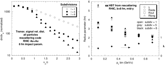
Figure 19: Subdivision test of the HRM code, showing transverse signal velocity distribution and pion HBT parameters vs. $p_{T}$ for $b=8$ fm centrality and subdivisions 1, 5, and 8.

3.4 Comparison of HRM with AGS ($\sqrt{s}\sim 2$ GeV/nucleon) and SPS ($\sqrt{s}\sim 20$ GeV/nucleon) experiments

Having discussed some of the features of the HRM, comparisons between HBT results from the HRM with AGS and SPS experiments are now presented below in Figures 20-23.

Figure 20 shows a comparison between boson source parameters from the HRM (triangles) with those from the fixed-target central collisions 200 GeV/nucleon S+Pb measured by SPS experiment NA44[11, 31] and 14.6 GeV/nucleon Si+Au from the AGS experiment E859/E866[32] (circles). Both experiments are based on small acceptance magnetic spectrometers with good particle identification allowing them both to also carry out HBT measurements with kaon pairs as well as pion pairs as shown in the figure. As seen, NA44 also measured pion source parameters with a low-$p_{T}$ cut ($<p_{T}>\sim 150$ MeV/c) and a high-$p_{T}$ cut ($<p_{T}>\sim 450$ MeV/c) on the pion momentum. The HRM is seen to follow the trends of the data rather well, predicting the decrease in the source parameters with the higher pion momentum cut (NA44) and for both experiments predicting smaller source parameters extracted from the kaon-pair HBT measurements. In the context of the HRM, the explanation for the smaller parameter sizes extracted used kaon pairs is due to the generally smaller scattering cross sections for $K-\pi$ and $K-N$ reactions compared with those for pions. The dashed lines in the figure show the parameters extracted from HRM with rescattering turned off, showing that rescattering plays a crucial role in determining the scale and kinematic dependencies of the boson source parameters measured by HBT interferometry.

file=fighbt20.eps,width=7cm

Figure 20: Comparison between boson source parameters from the HRM (triangles) with those from SPS experiment NA44 and AGS experiment E859/E866 (circles). The dashed lines show the parameters extracted from HRM with rescattering turned off (From Ref.[26]).

Figure 21 presents a comparison between the HRM for various model configurations and HBT parameters extracted from fixed-target central 158 GeV/nucleon Pb+Pb collisions from SPS experiment NA49 (based on a large acceptance detector).[33] The dashed lines are projections of the NA49 data points to guide the eye. For the purposes of this figure, “IOC” refers to the use of Eq. (20) in the HRM (the normal method used) and “pill” refers to taking $t_{had}=0$ and $z_{had}$ uniformly distributed in the region $z=\pm 1$. As seen, the HRM predictions show robustness to the first three running configurations predictions being close to the measurements for the cases “IOC”, “pill”, and “pill(old)”, the latter being a calculation without resonances which accounts for the $\lambda$ parameter being unity for that case. The cases “IOC (pion gas)” and “IOC (no RS)”, referring to running the HRM code without kaons and nucleons and with rescattering turned off, respectively, are seen to deviate significantly from the measurements showing the importance of including the pions and kaons and rescattering in the calculations.

file=fighbt21.eps,width=10cm

Figure 21: Comparison between SPS experiment NA49 HBT results for $Pb+Pb$ with HRM for various model configurations. The dashed lines are projections of the NA49 data points to guide the eye (From Ref.[21]).

Figures 22 and 23 show more comparisons of HBT source parameters extracted from the HRM and the SPS NA49 and NA44 experiments. Figure 22 shows a comparison between HRM (points) and the trends of NA49 central 158 GeV/nucleon Pb+Pb experimental results[33] (dashed lines with same meaning as in Figure 21) for the $k_{T}$ dependence of the pion source parameters. Figure 23 compares an overview of HBT-extracted pion and kaon source parameters measured in the NA44 experiment[11, 34, 35, 36] with those calculated with the HRM. Although there are some minor disagreements, the HRM is seen overall to qualitatively describe the trends of the data for both experiments.

file=fighbt22.eps,width=10cm

Figure 22: Comparison between HRM (points) and the trends of NA49 $Pb+Pb$ experimental results (dashed lines with same meaning as in Figure 21) for the $k_{T}$ dependence of the pion source parameters (From Ref.[21]).

file=fighbt23.eps,width=10cm

Figure 23: Comparison between HRM calculations and boson source parameters extracted from the NA44 experiment (From Ref.[36]).

3.5 Comparison of HRM with RHIC ($\sqrt{s}\sim 130-200$ GeV/nucleon) experiments

Results from the first year of running of the Relativistic Heavy Ion Collider (RHIC) for Au+Au collisions at $\sqrt{s}=130$ GeV showed surprisingly large pion elliptic flow[37] and surprisingly small radii from two-pion HBT interferometry. [10, 38] Hydrodynamical models agreed with the large elliptic flow seen in the RHIC data[39] but significantly disagreed with the experimental HBT radii. [40] On the other hand, relativistic quantum molecular dynamics calculations which include hadronic rescattering, for example RQMD v2.4,[41] significantly under-predict the elliptic flow seen in the RHIC data[42] but predict pion HBT radii comparable to the data.[43] A calculation was made to extract HBT radii with a hydrodynamical model coupled with a hadronic rescattering afterburner with the result that the HBT radii were significantly larger than measurements.[44] This situation lead to the first big mystery from RHIC, sometimes called the “HBT Puzzle.” It has even been suggested that one should call into question the current understanding of what information pion HBT measurements give.[45] In this context, the HRM model is compared with both elliptic flow and HBT measurements from RHIC to see if it can shed any light on this situation.

3.5.1 Elliptic flow results

The elliptic flow variable for a collision, $V_{2}$, is defined as[37]

$$V_{2}=<\cos(2\phi)>$$ (23)

$$\phi=\arctan(\frac{p_{y}}{p_{x}})$$

where $p_{x}$ and $p_{y}$ are the $x$ and $y$ components of the particle momentum, and $x$ is in the impact parameter direction, i.e. reaction plane direction, and $y$ is in the direction perpendicular to the reaction plane.

Figure 24 shows the $p_{T}$ dependence of $V_{2}$ for pions and nucleons extracted from the $b=8$ fm HRM calculation compared with the trends of the STAR measurements for $\pi^{+}+\pi^{-}$ and $p$ + $\overline{p}$ at $11-45\%$ centrality,[37] which roughly corresponds to this impact parameter.

file=fighbt24.eps,width=10cm

Figure 24: Calculations of $V_{2}$ from the HRM for $b=8$ fm for pions and nucleons compared with STAR measurements at 11-45% centrality. The plotted points with error bars are the HRM calculations and the lines show the trends of the STAR measurements. Average errors on the STAR measurements are $\leq 0.002$ for pions and $0.006$ for protons+antiprotons (From Ref.[22]).

Figure 25 compares the $p_{T}$ dependence of $V_{2}$ for kaons from the $b=8$ fm HRM calculation with the STAR measurements for ${K^{0}}_{s}$ at $11-45\%$ centrality.[46] As seen, the HRM calculation values are in reasonable agreement with the STAR measurements. The flattening out of the pion and nucleon $V_{2}$ distributions for $p_{T}>2$ GeV/c is consistent with that seen in STAR and PHENIX results for minimum-bias hadrons[47, 48] (the kaon $V_{2}$ calculation does not extend higher than 2 GeV/c in Figure 5 due to limited statistics). Thus, the same rescattering mechanism that can account for the radial flow seen in $m_{T}$ distributions, e.g. Figures 15 and 16, also is seen to account for the magnitude and $p_{T}$ dependence of the elliptic flow for pions, kaons, and nucleons.

file=fighbt25.eps,width=10cm

Figure 25: Calculation of $v_{2}$ from HRM for kaons at $b=8$ fm compared with STAR measurements for ${K^{0}}_{s}$ at 11-45% centrality (From Ref.[22]).

3.5.2 “Year-1” HBT results

The pion source parameters extracted from HBT analyses of HRM calculations for three different impact parameters, $b=0$, $5$, and $8$ fm, are compared with STAR $\pi^{-}$ measurements at three centrality bins[10] in Figure 26. Note that the PHENIX experiment HBT results[38] are in basic agreement with the STAR results. The STAR centrality bins labeled “3”, “2”, and “1” in the figure correspond to $12\%$ of central, the next $20\%$, and the next $40\%$, respectively. These bins are roughly approximated by the impact parameters used in the HRM calculations, i.e. the average impact parameters of the STAR centrality bins are estimated to be within $\pm 2$ fm of the HRM calculation impact parameters used to compare with them. In the left panel, the centrality dependence of the HBT parameters is plotted for a $p_{T}$ bin of $0.125-0.225$ GeV/c. In the right panel, the $m_{T}$ dependence of the HBT parameters is plotted for centrality bin 3, for the STAR measurements, or $b=0$ fm, for the HRM calculations. Although there are differences in some of the details, the trends of the STAR HBT measurements are seen to be described rather well by the HRM calculation.

file=fighbt26.eps,width=12cm

Figure 26: Comparison of HBT source parameters from HRM with STAR measurements as a function of centrality bin (see text) and $m_{T}$. The STAR measurements are the solid symbols and the rescattering calculations are the open symbols. The errors on the STAR measurements are statistical+systematic (From Ref.[22]).

3.5.3 Azimuthal HBT results

It was first shown experimentally at the AGS that looking at the azimuthal dependence of HBT with respect to the reaction plane can give another handle on the space-time evolution of the pion source.[49] For central collisions with vanishing impact parameter ($b\sim 0$) one would expect no azimuthal dependence since the initial collision is symmetric about the beam axis. However, for non-central ($b>0$) collisions, a definite initial asymmetry with respect to the beam axis will exist which may be reflected in the extracted HBT source parameters. The STAR collaboration has recently published experimental results on the azimuthal dependence of pion HBT parameters in central and non-central RHIC collisions.[50] Preliminary calculations have been made with the HRM to extract azimuthal HBT parameters to compare with the STAR results. These comparisons are shown in Figures 27 and 28 below. In Figure 27 the azimuthal dependence of HBT parameters is shown for $b=0$ fm rescattering model calculations compared with results from STAR central collisions ($0-5\%$ centrality). As seen for both the calculation and data, no oscillations occur with respect to $\phi$ for any of the parameters except the cross-term parameter, $R_{outside}^{2}$, as would be expected for an azimuthally symmetric system. Figure 28 shows a similar comparison for $b=4$ fm calculations and STAR medium-central collisions ($10-20\%$ centrality). As would be expected, the non-central collisions break the azimuthal symmetry of the pion source and oscillations are now seen in all parameters. The calculations are seen to be in reasonable qualitative agreement with the data.

Figure 27: Azimuthal pion HBT parameters from the rescattering model with $b=0$ fm centrality compared with central STAR results

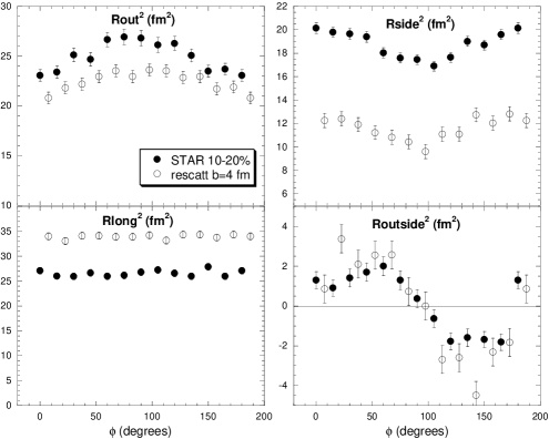
Figure 28: Azimuthal pion HBT parameters from the rescattering model with $b=4$ fm centrality compared with medium-central STAR results

3.5.4 Discussion of RHIC results

As shown above, the elliptic flow as well as the features of the HBT measurements at RHIC can be adequately described by HRM with the hadronization model parameters given earlier in Table I. The results of the calculations are found to be sensitive to the value of $\tau_{had}$ used, as was studied in detail for SPS HRM calculations.[21] For calculations with $\tau_{had}>1$ fm/c the initial hadron density is smaller, fewer collisions occur, and the rescattering-generated flow is reduced, reducing in magnitude the radial and elliptic flow and most of the HBT observables. Only the HBT parameter $R_{Long}$ increases for larger $\tau_{had}$ reflecting the increased longitudinal size of the initial hadron source, as seen in Eq. (20). One can compensate for this reduced flow in the other observables by introducing an ad hoc initial “flow velocity parameter”, but the increased $R_{Long}$ cannot be compensated by this new parameter. In this sense, the initial hadron model used in the present calculations with $\tau_{had}=1$ fm/c and no initial flow is uniquely determined with the help of $R_{Long}$.

At this point, one can consider the physical significance of the HRM in two different ways. The first way is to accept that it is physically valid in the time range where hadronic rescattering should be valid, e.g. for times later than when the particle density reaches about 1 $fm^{-3}$, and to take the initial state hadronization model as merely a parameterization useful to fit the data. Considering the calculation this way, one can at least expect to gain an insight into the phase-space configuration of the system relatively early in the collision (in the calculation 1 $fm^{-3}$ occurs at a time 4 fm/c after hadronization). The second way to consider the calculation is to see if it is possible to also physically motivate the initial state hadronization model. An attempt to do this is given below.

In order to consider the present initial state model as a physical picture, one must assume: 1) hadronization occurs very rapidly after the nuclei have passed through each other, i.e. $\tau_{had}=1$ fm/c, 2) hadrons or at least hadron-like objects can exist in the early stage of the collision where the maximum value of $\rho$ approaches 8 GeV/$fm^{3}$, and 3) the initial kinetic energies of hadrons can be large enough to be described by $T=300$ MeV in Equation 1.

Addressing assumption 2) first, in the calculation the maximum number density of hadrons at mid-rapidity at $t=0$ fm/c is 6.8 $fm^{-3}$, rapidly dropping to about 1 $fm^{-3}$ at $t=4$ fm/c. Since most of these hadrons are pions, it is useful as a comparison to estimate the effective volume of a pion in the context of the $\pi-\pi$ scattering cross section, which is about 0.8 $fm^{2}$ for s-waves.[28] The “radius” of a pion is found to be 0.25 fm and the effective pion volume is 0.065 $fm^{3}$, the reciprocal of which is about 15 $fm^{-3}$. From this it is seen that at the maximum hadron number density in the calculation, the particle occupancy of space is estimated to be less than $50\%$, falling rapidly with time. One could speculate that this may be enough spacial separation to allow individual hadrons or hadron-like objects to keep their identities and not melt into quark matter, resulting in a “super-heated” semi-classical gas of hadrons at very early times, as assumed in the present calculation.

Since the calculation takes the point of view of being purely hadronic, it is instructive to consider assumptions 1) and 3) in the context of the Hagedorn thermodynamic model of hadronic collisions. [51] According to Hagedorn, the mass spectrum of hadrons of mass m increases proportional to $\exp{(m/T_{0})}$ in hadronic collisions, where $T_{0}=160$ MeV is the limiting temperature of the system. This seems to contradict the value $T=300$ MeV needed in the present case in Eq. (18) to describe the data. The Hagedorn model assumes that a) the system comes to equilibrium and b) the details of particle production via direct processes and through resonance decay average out. Neither of these assumptions is necessarily guaranteed at very early times in the collision. The use of the thermal functional form, Equation 1, to set up the initial transverse momenta of the hadrons in the present calculations is convenient but not required. For example, the exponential form $\exp{(-m_{T}/T_{e})}$ (where $T_{e}$ is a slope parameter) which does not describe thermal equilibrium, could have equally well been used. This exponential form of the transverse mass distribution was successfully used previously in rescattering calculations to describe SPS data.[26, 27]

Assumption 1) can also be motivated by the Color Glass Condensate model.[52, 53] In the usual version of this picture, after the collision takes place the Color Glass melts into quarks and gluons in a timescale of about 0.3 fm/c at RHIC energy, and then the matter expands and thermalizes into quark matter by about 1 fm/c. In the context of the HRM calculations, it is tempting to modify the collision scenario such that instead of the Color Glass melting into quarks and gluons just after the collision, the sudden impact of the collision “shatters” it directly into hadronic fragments on the same timescale as in the parton scenario due to the hadronic strong interactions.

3.6 Predictions from HRM for LHC ($\sqrt{s}\sim 5500$ GeV/nucleon) experiments

Since it has been found that the predictions from HRM agree rather well with AGS, SPS, and RHIC measurements, it is interesting to use this model to make similar predictions for Pb+Pb collisions at the LHC. Preliminary calculations for the LHC have been carried out with HRM, the results from which are shown below. In performing LHC calculations, the following parameters were used in the code: 1) a collision impact parameter of $b=8$ fm, 2) an initial temperature parameter of $500$ MeV, 3) a hadronization proper time for the initial system of 1 fm/c, 4) a $dn/dy$ at mid-rapidity for central collisions for all particles of 4000, and 5) an initial rapidity width of 4.2. These parameters were judged to be reasonable guesses to simulate LHC Pb+Pb collisions. They at least satisfy the self-consistency check that summing over the energy of all particles in an event at the end of the calculation agrees with the input total energy of a LHC Pb+Pb collision with an impact parameter of $b=8$ fm. An impact parameter of $b=8$ fm was chosen for the present preliminary study both to obtain non-negligible elliptic flow values and for calculational convenience (even for this impact parameter the cpu time used by the code for each LHC Pb+Pb event was about 60 hours). For item 3) above, the hadronization proper time was taken to be the same as was used in the SPS and RHIC calculations. Results of these calculations are compared with similar calculations at $b=8$ fm centrality for RHIC Au+Au collisions and are shown in Figures 29, 30, and 31. All of these results are obtained at mid-rapidity, i.e $-2<y<2$.

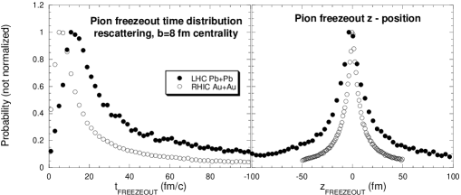
Figure 29: Pion freezout time and z-position distributions for LHC Pb+Pb and RHIC Au+Au for $b=8$ fm centrality collisions at mid-rapidity from HRM.

Figure 29 shows the pion freezeout time and z-position distributions for LHC Pb+Pb and RHIC Au+Au from HRM. As seen, the average pion freezeout time and z-position for LHC are about twice as large as those for RHIC. Although the tails of the freezeout time distributions extend beyond 100 fm/c, the peaks for the LHC and RHIC occur at fairly short times in the collision, at about 5 fm/c and 10 fm/c, respectively. Thus, effects from earlier times in general have the greatest influence on the results from these calculations.

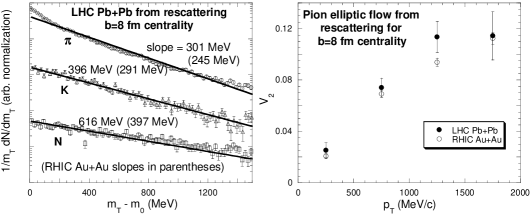
Figure 30: $m_{T}$ distribution and pion elliptic flow predictions for LHC Pb+Pb compared with RHIC Au+Au for $b=8$ fm centrality collisions at mid-rapidity from HRM. Note that in the plot on the left, corresponding RHIC slope parameters from HRM are show in parentheses for comparison with the LHC values.

Figure 30 shows the radial and elliptic flow predictions for LHC Pb+Pb compared with RHIC Au+Au from HRM. As seen in the $m_{T}$-distribution plot on the left, although all species of particles start from a common temperature in the calculation, after rescattering the exponential slope parameters follow the usual radial flow pattern of $slope(\pi)<slope(K)<slope(N)$ for both LHC and RHIC. The slopes are seen to be consistently larger at LHC than RHIC, as well as for the degree of radial flow which is built up. Looking at the plot of pion elliptic flow vs. $p_{T}$ on the right, it is seen that LHC and RHIC give about the same values. This is due to the elliptic flow stabilizing at a very early stage in the HRM calculation.

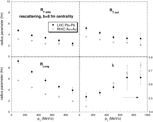
Figure 31: Pion HBT predictions for LHC Pb+Pb compared with RHIC Au+Au for $b=8$ fm centrality collisions at mid-rapidity from HRM.

Figure 31 shows the pion HBT parameters vs. $p_{T}$ for LHC Pb+Pb compared with RHIC Au+Au from HRM. The transverse radius parameters, $R_{Tside}$ and $R_{Tout}$, are seen to be somewhat larger and show a stronger $p_{T}$ dependence for LHC as compared with RHIC. The longitudinal radius parameter, $R_{Long}$ is seen to be significantly larger for LHC as compared with RHIC, clearly reflecting that the pion freezeout times at LHC are twice as long as at RHIC according to HRM. The $\lambda$ parameter is seen to increase with increasing $p_{T}$ in the same way for both LHC and RHIC, reflected the reduced influence of long-lived resonances at the higher $p_{T}$ values.

Summarizing the results of this preliminary study, it is predicted from HRM that medium-peripheral ($b=8$ fm) LHC Pb+Pb collisions will produce more radial flow and larger HBT radii than the analogous RHIC Au+Au collisions, although elliptic flow and the $\lambda$ parameter values will look the same.

4 Summary

Over the past 25 years the HBT interferometry technique as applied to relativistic heavy ion collisions has evolved from being little more than a curiosity to becoming a standard tool applied by most RHI experiments to help understand their data. It has evolved in both its level of theoretical sophistication as well as in the level of precision at which HBT measurements can be carried out. The issue still remains of how to physically interpret the HBT observables which are measured. As is the clear theme of the present review, hadronic scattering models provide a means of addressing this issue of interpretation. Because of their success in describing the behavior of experimental HBT parameters, in addition to other measured observables such as the radial and elliptic flow, such models can be used in conjunction with experiments to view relativistic heavy ion collision at an earlier stage prior to the randomizing effects of the rescattering process. It will be more than interesting to carry out HBT measurements at the LHC in several years and thus to see if nature presents us with a host of new HBT puzzles to solve.

References

- [1] M. A. Lisa, S. Pratt, R. Soltz and U. Wiedemann, arXiv:nucl-ex/0505014 (2005).
- [2] U. W. Heinz and B. V. Jacak, Ann. Rev. Nucl. Part. Sci. 49, 529 (1999).
- [3] R. Hanbury-Brown and R. Q. Twiss, Nature 177, 27 (1956).
- [4] Hanbury-Brown attended the CRIS’98 (2nd Catania Relativistic Ion Studies) conference on HBT in RHI in Catania in 1998 as the honored speaker of the conference (the author had the privilege of talking with him there). He remarked that before attending this conference he had no idea that his technique was used outside the field of astronomy.
- [5] R. Hanbury-Brown and R. Q. Twiss, Nature 178, 1046 (1956).
- [6] R. Hanbury-Brown and R. Q. Twiss, Phil. Mag. 45, 663 (1954).
- [7] Hanbury-Brown mentioned his measurement of Alpha Centauri during a coffee break at the CRIS’98 conference. He said that he was surprised that the HBT signal was half of what he expected from observing its brightness with other methods (e.g. a single photomultiplier tube). At first, he thought there was something wrong with the detector setup, but finally convinced himself that a binary star should give half the expected HBT signal. He assigned the derivation of this to us as a homework problem, and this is my solution to it.
- [8] G. Goldhaber, S. Goldhaber, W. Lee, and A. Pais, Phys. Rev.120, 300 (1960).
- [9] M. Gyulassy, S. K. Kauffmann, and L. W. Wilson, Phys.Rev.C 20, 2267 (1979).
- [10] C. Adler et al. [STAR Collaboration], Phys. Rev. Lett. 87, 082301 (2001).
- [11] H. Beker et al. [NA44 Collaboration], Phys.Rev.Lett. 74, 3340 (1995).
- [12] S. Pratt, T. Csorgo, and J. Zimanyi, Phys. Rev. C 42, 2646 (1990)
- [13] B. Mueller, Nucl.Phys. A590 ,3c (1995); E. Laermann, Nucl.Phys. A610, 1c (1996).
- [14] H. Satz, Nucl.Phys. A590, 63c (1995); NA50 Collaboration, M. Gonin et al., Nucl.Phy. A610, 404c (1996).
- [15] J. Cugnon and R. M. Lombard, Phys. Lett. B134, 392 (1984).
- [16] J. Cugnon et al., Nucl. Phys. A355, 477 (1981).
- [17] T. J. Humanic, Phys. Rev. C 34, 191 (1986).
- [18] W. A. Zajc et al., Phys. Rev. C 29, 2173 (1984).
- [19] D. Beavis et al., Phys. Rev. C 27, 910 (1983).
- [20] D. Beavis et al., Phys. Rev. C 28, 2561 (1983).
- [21] T. J. Humanic, Phys. Rev. C 57, 866 (1998).
- [22] T. J. Humanic, Nucl.Phys. A715,641(2003).
- [23] M. Herrmann and G. F. Bertsch, Phys. Rev. C 51, 328 (1995).
- [24] J. D. Bjorken, Phys. Rev. D 27, 140 (1983).
- [25] U. Goerlach et al. [HELIOS Collaboration], Nucl. Phys. A 544, 109C (1992).
- [26] T. J. Humanic, Phys.Rev.C 53, 901 (1996).
- [27] T. J. Humanic, Phys. Rev. C 50, 2525 (1994).
- [28] M. Prakash, M. Prakash, R. Venugopalan and G. Welke, Phys. Rept. 227, 321 (1993).
- [29] Denes Molnar and Miklos Gyulassy, Phys. Rev. C 62, 054907 (2000).
- [30] T. J. Humanic, arXiv:nucl-th/0301055v1 (2003).
- [31] H. Beker et al. NA44 Collaboration], Z. Phys. C 64, 209 (1994).
- [32] V. Cianciolo et al. [E859/E866 Collaboration], Nucl. Phys. A590, 459c (1995).
- [33] K. Kadija et al. NA49 Collaboration], Nucl. Phys. A610, 248c (1996); H. Appelshuser, Ph.D. thesis, University of Frankfurt (1996).
- [34] A. Franz et al. [NA44 Collaboration], Nucl.Phys. A610, 240c (1996).
- [35] I. G. Bearden et al. [NA44 Collaboration], Phys. Rev. C 58, 1656 (1998).
- [36] T. J. Humanic, Nucl. Phys. A661, 431c (1999).
- [37] C. Adler et al. [STAR Collaboration], Phys. Rev. Lett. 87, 182301 (2001).
- [38] K. Adcox et al. [PHENIX Collaboration], arXiv:nucl-ex/0201008.
- [39] P. F. Kolb, J. Sollfrank and U. W. Heinz, Phys. Lett. B 459, 667 (1999).
- [40] D. H. Rischke and M. Gyulassy, Nucl. Phys. A 608, 479 (1996).
- [41] H. Sorge, H. Stocker and W. Greiner, Annals Phys. 192, 266 (1989).
- [42] H. Sorge, Phys. Rev. C 52, 3291 (1995).
- [43] D. Hardtke and S. A. Voloshin, Phys. Rev. C 61, 024905 (2000).
- [44] S. Soff, S. A. Bass and A. Dumitru, Phys. Rev. Lett. 86, 3981 (2001).
- [45] M. Gyulassy, arXiv:nucl-th/0106072.
- [46] J. Adams et al. [STAR Collaboration], Phys. Rev. Lett. 92, 052302 (2004).
- [47] R. J. Snellings [STAR Collaboration], Nucl. Phys. A 698, 193 (2002).
- [48] W. A. Zajc et al. [PHENIX Collaboration], Nucl. Phys. A 698, 39 (2002).
- [49] M. A. Lisa et al. [E895 Collaboration], Phys. Lett. B 496, 1 (2000).
- [50] J. Adams et al. [STAR Collaboration], Phys. Rev. Lett. 93, 012301 (2004).
- [51] R. Hagedorn, Nucl. Phys. B 24, 93 (1970).
- [52] L. D. McLerran, arXiv:hep-ph/0202025.
- [53] A. Kovner, L. D. McLerran and H. Weigert, Phys. Rev. D 52, 6231 (1995).