A COMPLEX SHELL MODEL REPRESENTATION INCLUDING ANTIBOUND STATES

Abstract

A generalization of the Complex Shell Model formalism is presented which includes antibound states in the basis. These states, together with bound states, Gamow states, and the continuum background, represented by properly chosen scattering waves, form a representation where all states are treated on the same footing. Two-particle states are evaluated within this formalism and observable two-particle resonances are defined. The formalism is illustrated in the well known case of ¹¹Li in its bound ground state and in ⁷⁰Ca(gs), which is also bound. Both cases are found to have a halo structure. These halo structures are described within the generalized Complex Shell Model. We investigated the formation of two-particle resonances in these nuclei, but no evidence of such resonances was found.

I Introduction

One of the most intriguing developments in nuclear physics is the disclosure of antibound states as important building blocks to induce the appearance of halos in exotic nuclei. The explanation of halos as well as the description of the behaviour of exotic nuclei, which live a short time and therefore their dynamics is governed by process occuring in the continuum part of the spectrum, requires the introduction of new and powerful models to take into account the complicated interplay among different degrees of freedom that produce weakly bound and resonant states. Such models appeared as soon as the experimental evidence in exotic nuclei provided a variety of features which could not be explained by standard approaches like the shell model using harmonic oscillator representations.

The lively activity that characterizes this field can be attested by the rapid development that is taken place. It would be outside the scope of this paper to assess those models. One of the first reviews is still rather recent zhu . Since then much have been published. In light nuclei a concise but clear account is in Ref. gar . A more comprehensive treatment (including abundant references) can be found in Ref. suz . The Continuum Shell Model is also been applied for this purpose oko .

Among the attemps to describe the structure of rare nuclei the Complex Shell Model method (CXSM) rsm ; mic ; cxsm presents the advantage of incorporating on an equal footing bound single-particle states as well as resonances and the non-resonant continuum. Recently, in a short publication ant , even the elusive antibound states have been included in the CXSM basis. The purpose of this paper is to present in a more extensive fashion the work of Ref. ant . At the same time the influence of the different ingredients that determine the importance of the antibound state will be appraised by analyzing realistic situations. The formalism is in Section II, applications are in Section III and a summary and conclusions are in Section IV.

II Formalism

Although the formalism to be used here was given before, we will present it again with some detail for clarity of presentation and also because we will deal with unfamiliar quantities like antibound states and complex probabilities which we would like to clarify from the outset. In addition we would like to display in the presentation the advantages of working in the complex energy plane, with its implicit loose of familiar quantum mechanical concepts, as compared with standard representations on the real energy axis.

With this in mind we start by pointing out that the study of processes taking part in the continuum part of the spectrum may require, by the very nature of the problem, a time dependent formalism. Therefore the quantum description of the system may become a very hard undertaking. In fact it may even become an impossible task, since the dynamics of the problem may be very sensitive to the initial conditions and the system can easily precipitate into a chaotic regime. But there are exceptions to this setting. Thus, the spectrum corresponding to a system of free particles is a monotonous and continuum function of the energy as determined by the kinetic motion of the particles, and the time-independent Schrödinger equation is suitable to explain this system.

A not so clear situation where time-independent formalisms can be applied occurs even if the particles start to interact with each other under the influence of a central field. Here the continuum may acquire features which depart from the monotony of the kinetic energy spectrum. The physical meaning of these structures is that due to the interactions the system remain in a certain configuration during a time, i. e. within an energy interval. In other words, the system is trapped by a barrier erected by the interactions as well as by the centrifugal motion. The structures appearing on the continuum background are the resonances. If the barrier is high enough the system will remain during a long time in a localized region of space and the dynamics of the process can be studied within stationary formalisms. The question that one may ask is what is meant by ”long time” or ”barrier high enough”. This question is irrelevant in radioactive decay, since measurable mean lives correspond to very narrow resonances. Thus, for the shortest measurable radioactive decay (i. e. the widest measurable resonance) the mean life is at present $T\approx 10^{-12}$ sec and the width is, according to the uncertainty relation, $\Gamma=6.6\times 10^{-10}$ MeV. Therefore in this time-energy scale the nucleus lives a long time before decaying and one may assume that the process is stationary. But this is not the case in all processes occurrying in the continuum. In particular the formation of halos could proceed through wide resonances where even the proper continuum plays a role, as we will see in the next Section. On the other hand, if the resonance is very wide the halflive is very short, indicating that the system is not trapped in a barrier during a long time and the process can not be considered stationary. One can still try to solve the time-independent Schrödinger equation in this situation to gain insight into the limitations of the problem. Since the system is not trapped by a barrier high enough all or parts of its components will soon depart from the rest. To study this situation in a many-body case is a difficult task. We therefore start from the simplest case, that is a particle moving in a central field, as Gamow did in the beginning of quantum mechanics Gam28 .

II.1 The Berggren representation

We thus solve the time-independent Schrödinger equation imposing to the wavefunction $w_{n}(r,k_{n})$ regularity at origin and outgoing boundary conditions (the particle departs from the origin), i. e. we require Pei38

$$\lim_{r\to 0}w_{n}(r,k_{n})=0,~{}~{}~{}~{}\lim_{r\to\infty}w_{n}(r,k_{n})=N_{n}e^{ik_{n}r}$$ (1)

where $k_{n}$ is the asymptotic momentum of the state with energy eigenvalue $E_{n}$, i. e.

$$E_{n}=\frac{\hbar^{2}}{2\mu}k^{2}_{n}$$ (2)

The wavefunction $w_{n}(r,k_{n})$ thus defined can be considered a generalization of the definition of eigenvectors of the single particle Schrödinger equation. The eigenvalues $E_{n}$ can now be complex. Writing

$$k_{n}=\kappa_{n}+i\gamma_{n}$$ (3)

the eigenvectors belonging to those eigenvalues can be classified in four classes, namely: (a) bound states, for which $\kappa_{n}$=0 and $\gamma_{n}>0$; (b) antibound states with $\kappa_{n}$=0, $\gamma_{n}<0$; (c) decay resonant states with $\kappa_{n}>0$, $\gamma_{n}<0$ and (d) capture resonant states with $\kappa_{n}<0$, $\gamma_{n}<0$. From Eq. (1) one sees that only the bound state wave functions do not diverge.

The imaginary part of the energy of the states (c) was interpreted by Gamow as minus twice the width of the resonance Gam28 and therefore these states are usually called Gamow resonances. However, we will make a distinction between real resonances, having physical meaning, and other ”resonances” which are generally wide and therefore do not correspond to any particular observable state. To avoid having to distinguish between these different situations any time we refer to the four classes of outgoing states described above we will refer to them in general as ”poles”, since they are the poles of the Green function n66 and, therefore, of the S-matrix.

With the standard definition of scalar product only the bound states can be normalized in an infinite interval. Therefore this definition has to be generalized in order to be able to use the generalized ”eigenvectors”. This can only be done if one uses a bi-orthogonal basis. As we will see, a consequence of this generalization is that the scalar product between two functions is not the integral of one of the functions times the complex conjugate of the other but rather times the function itself, and one has to apply some regularization method for calculating the resulting integrals. We will perform this task by using the complex rotation method Gya71 .

Berggren found that some of these complex eigenvectors (bound states and decaying resonances) can be used to express the Dirac $\delta$-function b68 . We will show the main points of his derivation since we will come back to it frequently.

One can write the Dirac $\delta$-function on the real energy axis, i. e. within a quantum mechanical framework, as n66

$$\delta(r-r^{\prime})=\sum_{n}w_{n}(r)w_{n}(r^{{}^{\prime}})+\int_{0}^{\infty}dEu(r,E)u(r^{{}^{\prime}},E)$$ (4)

where $w_{n}(r)$ are the bound states wavefunctions and $u(r,E)$ are scattering states. The integration contour is along the real energy axis. Notice that it appears the wavefunction times itself, and not times its complex conjugate, although (4) is a distribution to be applied on the Hilbert space. This is because for both bound states and scattering states on the real energy axis one can choose the phases such that the wavefunctions are real.

Berggren extended the expression (4) by prolonging the integration contour to the complex energy plane. Using the Cauchy theorem one gets b68

$$\delta(r-r^{\prime})=\sum_{n}{\tilde{w}^{*}_{n}(r)}w_{n}(r^{{}^{\prime}})+\int_{L^{+}}dE{\tilde{u}^{*}(r,E)}u(r^{{}^{\prime}},E)$$ (5)

where the sum runs over all the bound states plus the complex poles which lie between the real energy axis and the integration contour $L^{+}$, as shown in Fig. 1. This contour may have any form one wishes but, since it is a topological deformation of the real energy axis, it should be a continuum curve that starts in the origin, i. e. at $(0,0)$, and end at infinite, i. e. at $(\infty,0)$. However, as in any shell model calculation one cuts the basis at certain maximum energy which in the Figure is the point $(c,0)$.

Figure 1: Integration contour $L^{+}$ in the complex energy plane as defined by the vertex points $V_{i}$. The open circles represent the Gamow resonances to be included in the sum of Eq. (5) while the solid circles are those which are excluded. The vertex $(c,0)$ corresponds to the energy cut-off point $c$.

The wavefunction $\tilde{w}_{n}(r)$ is the mirror state of $w_{n}(r,k_{n})$, i. e. the solution with $\tilde{k}_{n}=-k^{*}_{n}$. Therefore $\tilde{w}^{*}_{n}(r)=w_{n}(r)$. The same is valid for the scattering state $u(r,E)$. We therefore indeed find that the internal product is the wavefunction times itself and not times its complex conjugate. This internal product is called Berggren metric.

The Gamow states enclosed by the contour $L^{+}$, plus the bound states and the scattering states on the contour, have been shown to form a complete set of single-particle states (Berggren representation) to describe many-body states in the complex energy plane l96 .

Discretizing the integral in Eq. (5) one obtains the set of orthonormal vectors $|\varphi_{j}\rangle$ forming the Berggren representation. These vectors include the set of bound and Gamow states, i . e. $\varphi_{p}(r)=\langle r|\varphi_{p}\rangle=\{w_{p}(r)\}$ and the discretized scattering states, i. e. $\varphi_{p}(r)=\langle r|\varphi_{p}\rangle=\sqrt{h_{p}}u(r,E_{p})$. The quantities $E_{p}$ and $h_{p}$ are defined by the procedure one uses to perform the integration. In the Gaussian method $E_{p}$ are the Gaussian points and $h_{p}$ the corresponding weights.

II.2 Berggren space and resonances

The representation above spans a space which is called Berggren space. Since within the metric defining the Berggren space the definition of scalar product does not include absolute values, one may have probabilities which are complex numbers. We thus find that forcing the time-dependent process of particles interacting in the continuum to be stationary one has to pay the price of having complex energies and complex probabilities. This is not as weird as it may sound, since we are now dealing with states lying in the complex energy plane which, in principle, do not have any physical meaning. This is a point which has produced some confusion already from the time of the first application of the theory nearly twenty years ago v87 . It is therefore important to clarify the meaning of this feature here where even another weird feature, namely antibound states, will be introduced.

Let us start by pointing out that the Berggren transformation leading to the representation (5) does not change in any way the meaning of the Dirac $\delta$-function. In particular, since on the real energy axis the wavefunctions can be chosen to be real, the results of a continuum shell model many-body calculation of quantities on the real energy axis (like e. g. sum rules or the energies of bound states) should coincide with the results provided by the same calculation using the Berggren metric with whatever contour one chooses provided that the resonances enclosed by that contour are also included. This is a very important property that will be used by us to check our results as well as our computer codes. Only for states lying in the complex energy plane the evaluated quantities will be unfamiliar, which is not surprising since these states lie outside the Hilbert space. Then the question is why one uses the Berggren space or, equivalently, which is the advantage of using the complex energy plane. This is a valid question which we will therefore answer in some detail.

In absence of any background the usual form of the S-matrix corresponding to a partial wave $(lj)$ in the neighborhood of an isolated resonance $n$ is

$${\cal S}_{nlj}(E)=\frac{E-E_{nlj}^{(0)}-\frac{i}{2}\Gamma_{nlj}}{E-E_{nlj}^{(0)}+\frac{i}{2}\Gamma_{nlj}}=\left[1-\frac{i\Gamma_{nlj}}{E-E_{nlj}^{(0)}+\frac{i}{2}\Gamma_{nlj}}\right]~{}.$$ (6)

where $E_{nlj}^{(0)}$ is the position and $\Gamma_{nlj}$ the width of the resonance. These are real positive numbers.

It is important to point out that Eq. (6) is valid only if the resonance is isolated. This condition is fulfilled for narrow resonances. In this case the residues ${\cal R}$ of the S-matrix is a pure imaginary number, i. e. ${\cal R}_{nlj}$=-i$\Gamma_{nlj}$, as readily follows from Eq. (6).

The cross section corresponding to the scattering of a particle at an energy close to the isolated resonance acquires the form

$$\sigma_{lj}(E)=(2l+1)\frac{\pi}{k^{2}}\frac{\Gamma^{2}_{lj}}{(E-E^{(0)}_{lj})^{2}+(\Gamma_{lj}/2)^{2}}~{},$$ (7)

This formula was derived by G. Breit and E. P. Wigner Bre36 to explain the capture of slow neutrons. It is one of the most successful expressions ever written in quantum physics, as shown by its extensive use in the study of resonances ever since. It was by comparing with experiment that Wigner interpreted the number $\Gamma$ as the width of the resonance. Since the imaginary part of the S-matrix pole is -$\Gamma/2$ (Eq. (6)), this interpretation coincided with the Gamow interpretation of the width. It is often assumed that the value of $\Gamma$ thus defined is the width of the resonance if it is narrow, i. e. if $\Gamma$ is small enough. However, a state having a very small (in absolute value) part of the energy is not necessarily a physically meaningful resonance. For instance in the CXSM calculation of two-particle resonances there are states lying very close to the real energy axis which form part of the continuum background since they are induced by basis vectors belonging to the continuum contour cxsm . But besides this objection one my ask what it is meant by ”large” and ”small” width even in the case of a pure Gamow pole.

To avoid these objections and to get a more precise definition of a resonance we notice that the condition that the resonance is isolated is equivalent to the requirement that the residues of the S-matrix should be a pure imaginary number. This criterion was used in Ref. Ver95 to evaluate partial decay widths corresponding to the emission of neutrons from giant resonances. It was thus found that only in a few cases the residues of the S-matrix was a pure imaginary number. Usually that quantity was complex and therefore devoided of any physical meaning. Yet, in some circunstances one can show that the imaginary part of the width thus evaluated (that is, as $\Gamma_{nlj}$=2i${\cal R}_{nlj}$) indicates that the lifetime of the resonance is too short and that it can be considered as a part of the background b78 .

The important conclusion of this discussion is that the imaginary part of the energy, which in some cases can even be evaluated analytically Hum61 , is not in itself related to the width.

A more precise definition of a resonance can be obtained by requiring that the corresponding complex pole posseses some physical attribute. As already pointed out, a measurable resonance corresponds to a process in which the system is trapped inside a barrier during a long time. One can therefore define a resonance according to its degree of localization inside the nuclear volume. This criterion will be very important to identify the two-particle resonances to be studied in the applications. Thus, we will evaluate all resonances that can be built within our Berggren single-particle representation and give physical meaning to the ones with wavefunctions showing localization properties within the nuclear volume. But it is important to point out that although this criterion is more accurate to define a resonance in comparisson to e. g. the one based on the value of the imaginary part of the energy, the very nature of the problem hinders an exact formulation of a criterion to define a resonance in the framework of a time independent formalism. Therefore even our criterion of defining a resonance according to its localization features has to be considered approximate.

The developing of a resonance depends upon the central mean field as well as the two body residual interaction acting upon the basis elements. As in any shell-model calculation the interplay among these elements induces the correlated states which, in our case, include resonances, bound and antibound states. One thus expects that correlated narrow resonances may be induced not only by bound states and narrow resonances but also by wide resonances, antibound states and even the continuum itself. The evolution of this complicated process as a function of the interactions as well as the dimension of the basis (including the energy cut-off that defines the representation) can clearly be seen in the complex energy plane, since the location of the complex energies corresponding to the resonances are just points in the two-particle complex plane. This would be very difficult to do on the real energy axis, since here the wavefunctions corresponding to wide resonances cannot be easily diferentiated from those corresponding to the continuum background. This is an important advantage of using the complex energy plane. We will come back to this point below.

The two-particle shell-model equations have the standard form, except the metric, i. e.

$$(\omega_{\alpha}-\epsilon_{i}-\epsilon_{j})X(ij;\alpha)=\sum_{k\leq l}<\tilde{kl};\alpha|V|ij;\alpha>X(kl;\alpha)$$ (8)

where $\alpha$ labels two-particle states and $i,j,k,l$ label single-particle states. As in Eq. (5) tilde denotes mirror states.

In principle the zeroth order energies $\epsilon_{i}+\epsilon_{j}$ would cover the whole two-particle energy plane (since $\epsilon$ is actually a continuous variable) and the correlated state would thus be immersed in a background of uncorrelated states. However, one can avoid this problem by chosen suitable contours cxsm .

A convenient fashion of solving Eq. (8) is by using a separable two-body interaction. One thus obtains the dispersion relation cxsm

$$-\frac{1}{G_{\alpha}}=\sum_{i\leq j}\frac{f^{2}_{\alpha}(ij)}{\omega_{\alpha}-\epsilon_{i}-\epsilon_{j}}$$ (9)

where $G_{\alpha}$ is the interaction strength and $f_{\alpha}(ij)$ is the matrix element of the field defining the interaction. We will choose for this field the derivative of the Woods-Saxon potential given by

$$F(r)=\frac{f_{0}}{1+exp(r-R^{\prime})/a^{\prime}}$$ (10)

i. e. the field $f$ is

$$f(r)=-r\frac{dF(r)}{dr}$$ (11)

This choice of the field defining the two-body interaction differs from the one given in Refs. rsm ; cxsm , where the function $F$ was the Woods-Saxon potential used to evaluate the single-particle states. The reason of this is that now the central field defining the single-particle states contains also a Gaussian part, as we will see in the Aplications. With the present choice of the effective two-body interaction we are able to describe well experimental data, which is the main criterion used in Shell Model calculations to define the effective force.

The two-particle wavefunction can be written as

$$X(ij;\alpha)=N_{\alpha}\frac{f_{\alpha}(ij)}{\omega_{\alpha}-\epsilon_{i}-\epsilon_{j}}$$ (12)

where $N_{\alpha}$ is the normalization constant.

This form of the wavefunction shows clearly the problem one faces if no measure is taken to avoid the continuum background of uncorrelated states. As one chooses more points on the contour (thus improving, in principle, the procedure) the energy denominators corresponding to zeroth order states close to the energy $\omega_{\alpha}$ diminish and all wavefunctions tend to a common value, thus making impossible the identification of the correlated resonance.

This possibility of identifying individually the correlated states is another favorable feature of the complex energy plane. On the positive side of the real energy axis (i. e. on the continuum) there is no any unique correlated state because the poles of the two-particle Green function consist only of bound states, which lie on the physical $k$-sheet, or to resonances located on non-physical sheets kuk . Therefore one does not evaluate the energy (i. e. the position) of the resonances on the real energy axis but rather matrix elements of physical operators, like e. g. transition amplitudes, which increase (in absolute value) close to the resonance energy if the resonance is narrow enough be ; ebh . Such limitations do not exist in the complex energy plane. Instead, here one calculates all complex states but at the end, in order to assign physical meaning to those states as well as to compare with experiment, one chooses the integration contour as the real energy axis. At this point of the calculation the CXSM and standard methods like the Continuum Shell Model coincide. Only complex states showing the resonant features mentioned above (at energies around the real part of the complex energy) will have physical meaning. This is a manifestation that these states are localized inside the nuclear volume. The wavefunctions of non-localized states are small inside the nuclear volumen and their contribution to the matrix elements of physical operators is also small Bia01 . This feature will be illustrated below, where we will show localized as well as non-localized states.

Usually one chooses the contour of integration $L^{+}$ such that it encompasses only Gamow resonances, as in Fig. 1. However, in order to include antibound states, which is a major aim in this paper, one has to choose a generalized contour which should enclose not only the Gamow resonances but also the antibound states. Since for these states it is $k_{n}=-i\mid k_{n}\mid$ the corresponding energy is real and negative. As we will see, in some circumstances the antibound state has properties similar to the bound state. However, these states are fundamentally different. While the bound state wavefunction diminishes exponentially at large distances, the outgoing antibound state diverges exponentially.

The antibound states and resonances with $|\gamma_{n}|>\kappa_{n}$ were not included in the completeness relations originally suggested by Berggrenb68 . This was related to the regularization procedure used in that early work. The first attempt to generalize the completeness by including antibound states and all type of decaying resonances was in a pole RPA approximation ve89 in which the complex rotation in the radial distance was used as a regularization method. Later Berggren and Lind also discussed these type of generalized completeness relations be93 .

The single-particle states to be used in the applications will, therefore, be determined by the generalized contour shown in Fig. 2. The antibound state in this figure is the open circle on the real energy axis. Notice that the contour lies on the unphysical $E$-sheet since $Im(k)<0$.

Figure 2: Generalized integration contour $L^{+}$ in the complex energy plane as defined by the vertex points $V_{i}$. The open circles represent the antibound states and the Gamow resonances to be included in the Berggren representation, while the solid circles are those which are excluded. The open squares are the bound states, which have to be included independently of the integration contour that is chosen. The vertex $(c,0)$ corresponds to the energy cut-off point $c$.

We will perform the integration of the scattering states on the continuum contour by using the Gauss method. Assuming that there are $N_{p}$ poles within the chosen contour and $N_{g}$ Gaussian points in the integration procedure, the set of generalized basis states consists of $N=N_{p}+N_{g}$ elements. We will order this set such that $n=1,2,..,N_{p}$ labels the poles while $n=N_{p}+1,N_{p}+2,...,N$ labels the sattering states. The corresponding basis vectors are, with standard notation,

$$\varphi_{nljm}(\vec{r})=R_{nlj}(r)(\chi_{1/2}Y_{l}(\hat{r}))_{ljm}$$ (13)

It is important to point out that the Berggren metric affects only the radial part of these functions while the spin-angular part follows the usual Hilbert metric.

Summarizing this Section we have presented a representation that defines a space (Berggren space) which contains as a subspace the Hilbert space.

The formalism dealing with the many-body applications of the dynamics of a system within the Berggren space is called Complex Shell Model (CXSM).

The properties of the CXSM are perhaps bizarre and therefore it is important to clarify some points that we will use in the Applications.

The extension of the Berggren space is defined by the continuum contour. If it is chosen to be the real energy axis then the resulting CXSM coincides with the Shell Model. But as soon as the contour departs from the real energy axis then a new dimension appears in the Berggren space. However, whichever is the contour, the Shell Model remains a subspace of the CXSM. As a result, all the physical properties evaluated by the standard Shell Model has to coincide with the corresponding quantities evaluated within the CXSM. In particular, quantities like transition matrix elements or the angular momentum content of a state corresponding to bound states should be independent of the contour. For a complex state this may not be valid any more, since the state may be outside the Berggren space defined by the chosen contour. For instance (and perhaps obvious) the evaluation of those quantities in complex states by using the real energy axis as a contour would not be possible since the complex vector is outside the space spanned by the real energy-axis basis states (i. e. it is outside the Hilbert space).

Concepts like probabilities have no physical meaning for states outside the real energy axis, since they become usually complex quantities. However if the outgoing wavefunction corresponding to the complex poles show localization features then one may be able to consider the state as a resonance, for which the halflive can be defined.

These features will be discussed below.

III Applications

In this Section we will apply the formalism presented above to weakly bound nuclei. The most prominent of these nuclei is ¹¹Li, which we will also treat here but only as an example of the power of the method. Besides, we will show that in the neutron drip-line nucleus ⁷⁰Ca antibound states play a fundamental role to build the low energy spectrum.

In all cases the poles as well as the scattering states will be evaluated by using the high precision piecewise perturbation method tv2 .

III.1 The nucleus ¹¹Li

This nucleus has been a playing ground for methods and models invented to describe features associated to weakly bound nuclei, specially halos zhu ; gar ; suz . In the shell model approach one assumes that the odd proton occupying the shell $0p_{3/2}$ is inert and the low lying states can be described as two neutrons moving outside the core ⁹Li. Therefore the ground state of ¹¹Li is in this formalism the $0^{+}_{1}$ state coupled to the proton state $0p_{3/2}$, which is a pure spectator providing the angular momentum of the even-odd nucleus but which otherwise does not contribute in any way to the dynamics leading to the low lying states. The validity of this approach is justified by the strong correlations between the valence neutrons at large distance which determine the halo structure of the nucleus as well as the low energy spectrum be . Moreover, the disregard of the center of mass motion of the core, as we will do here, is an approximation which was found to work quite well ebh .

The core therefore is the nucleus ⁹Li, corresponding to N=6 neutrons, with the shells $0s_{1/2}$ and $0p_{3/2}$ frozen while the valence shells would be $0p_{1/2}$, $1s_{1/2}$ and perhaps even $0d_{5/2}$ and $0d_{3/2}$. The central field determining these single-particle states is often chosen as a Woods-Saxon potential. However, in order to reproduce the amount of s-wave content of the ground state wavefunction in ¹¹Li the depth of the potential was taken to be different for positive- and negative-parity states ant ; be ; ebh . Although with this choice one gets at the same time large bindings for the states $0s_{1/2}$ and $0p_{3/2}$ and weakly bound valence shells, it is an unpleasant feature to have to use a central potential which is state dependent. The valence shells are more sensitive to the value of the central potential close to the nuclear surface, indicating that a similar feature would be obtained if one uses a standard Woods-Saxon potential but with an additional central part of short range and large depth. This would insure a large binding for the states in the core while the valence shells would be loosely bound. With this in mind we chose a Woods-Saxon plus Gaussian central potential. The Woods-Saxon potential is defined by the parameters $V_{0}$=39.97 MeV, $V_{0}^{so}$=19.43 MeV, $r_{0}=r_{0}^{so}$=1.27 fm, $a=a^{so}$=0.67 fm, while the Gaussian potential is $V(Gauss)=-V_{g}\exp(-(r/a_{g})^{2})$ with $V_{g}$=663 MeV and $a_{g}$=0.26 fm. The resulting single-particle states are given in Table 1.

Table 1: Single-particle states used in the calculation of the two-neutron states in ¹¹Li. The energy $E_{n}$ and the wave number $k_{n}$ are related as in Eq 2. The $k_{n}-$value corresponding to the state $1s_{1/2}$ shows that this is an antibound state.

State	$E_{n}$ (MeV)	$k_{n}$ (fm-1)
$0s_{1/2}$	(-20.61,0)	(0,0.945)
$0p_{3/2}$	(-4.525,0)	(0,0.443)
$1s_{1/2}$	(-0.025,0)	(0,-0.033)
$0p_{1/2}$	(0.240,-0.064)	(0.103,-0.013)
$0d_{5/2}$	(4.334,-1.638)	(0.441,-0.081)
$0d_{3/2}$	(6.396,-9.898)	(0.628,-0.342)

One indeed sees that the shells $0s_{1/2}$ and $0p_{3/2}$ are deeply bound while the shell $1s_{1/2}$ lies close to threshold, but as an antibound state, as required by experimental evidence tz , and the shell $0p_{1/2}$ appears as a resonance at 240 keV and a width of 128 keV, as also required by experiment Boh97 . These two unbound states are the valence shells. They will determine the bound ground state of ¹¹Li, given to the three-body system consisting of the core, i. e. ⁹Li, and the two neutrons its Borromean character zhu .

We are assigning the features of a bound state to the shell $1s_{1/2}$ by labelling it with the principal quantum number $n=1$. This indicates that it has only one node (excluding the origin) although it is an antibound state. To show that this is indeed the case inside the nuclear volume, i. e. that this complex state is localized, we have plotted the radial part $R_{p}(r)$ (with $p\equiv 1s_{1/2}$) of the corresponding wavefunction in Fig. 3. In this Figure we also plotted the wavefunction corresponding to the equivalent bound state, i. e. with the same negative energy. To obtain the same energy as before but now bound (instead of antibound) we changed the depth of the Woods-Saxon potential to the value $V_{0}$=42.97 MeV (before it was $V_{0}$=39.97 MeV). The rest of the parameters defining the mean field (including the Gaussian part) are the same as before.

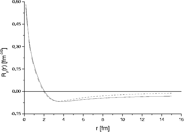
Figure 3: Radial wavefunction $R_{1s_{1/2}}(r)$ (Eq. (13)) corresponding to the bound (dashed line) and antibound (straight line) states in ¹⁰Li at (-0.025,0) MeV. The bound state was obtained by changing the depth of the Woods-Saxon potential, as explained in the text. The bound (antibound) wavefunction is purely real (imaginary).

With the usual definition of the nuclear radius, i. e. $R=r_{0}A^{1/3}$, $r_{0}$=1.25 fm, $A$=10, one gets $R$=2.69 fm, but in this neutron $l=0$ case there is not any barrier and the states lie so near the continuum threshold that the bound wavefunction extends far beyond the nuclear radius. This feature motivated the assumption of a weakly $1s_{1/2}$ bound state in ¹⁰Li when the halo structure of ¹¹Li was discovered. However, although great experimental efforts were made searching for such a state, no trace of it was ever found zhu . Finally, the $n+^{9}Li$ system was measured to have a large and negative scattering length (-17 fm) which prompted the realization that the state $1s_{1/2}$ indeed exists here at low energy, but actually as an antibound (or virtual) state tz .

In fact there is a similarity between bound and antibound states lying close to the continuum threshold. One sees in Fig. 3 that for these states the wavefunctions inside the nucleus are practically identical. They depart from each other only at large distances. Here the antibound wavefunction increases, eventually diverging. As mentioned above, the CXSM takes care of this divergence by regularizing all integrals using the complex rotation.

The localization of the antibound state can also be deduced from the behaviour of the corresponding scattering wavefunction on the real energy axis. At the energy $E=\hbar^{2}k^{2}/2\mu$ ($k$ real and positive) close to a bound or antibound state lying at a energy $E_{0}$ near threshold the scattering wavefunction can be written as mig ,

$$R_{l}(kr)\approx\sqrt{\frac{2k|k_{0}|}{k^{2}+|k_{0}|^{2}}}R_{l}(|k_{0}|r)$$ (14)

where $R_{l}(|k_{0}|r)$ is the scattering function at $positive$ energy $|E_{0}|$, although the wave numbers for the bound or antibound state are purely imaginary, i. e. $k_{0}=\pm i|k_{0}|$ respectively. That is, the energy values for these states are negative, $E_{0}<0$, but they lie on different energy sheets.

The expression (14) shows that close to threshold the radial shape of the scattering wavefunctions is independent upon the energy $E$ and the wave function depends on $E$ ($k$) only in its magnitude through the square root factor. This factor has its maximum at $k=|k_{0}|$ and therefore the large matrix elements in an energy region close to $E_{0}$ are induced by the S-matrix pole at imaginary $k_{0}$. In particular, as seen from Eq. (12), the two-body wavefunction in that energy region will be large on the real energy axis (i. e. within the continuum shell model). As we will see, this feature explains the large $l=0$ content of the ¹¹Li(gs) wavefunction. The remarkable point in this argument is that it does not matter whether the pole at $E_{0}<0$ corresponds to a bound or to an antibound state. Only the absolute value of $E_{0}$ is relevant and the effect is the same for both types of states, as expected from Fig. 3.

One should not take the similarity between bound and antibound states too far. To appraise this we notice that in the presence of a high barrier a bound state lying near the continuum threshold becomes a narrow Gamow resonance if one changes the central potential adequately, as we did above Bia01 . The imaginary part of the Gamow wavefunction thus obtained is small while the real part is very much alike the bound state in a range up to about twice the nuclear radius. Moreover, the Gamow wavefunctions of all narrow resonances, not only those lying near the continuum threshold, have negligible imaginary parts and real parts which are very similar, within the nuclear range as above, to the ones provided by a standard harmonic oscillator potential Bia01 . This feature explains why harmonic oscillator representations have been very successful in describing observable cluster decays, i. e. very narrow resonances Lov98 . But we want to stress, once again, that in general it is not the imaginary part of the energy which is a proper measure of the width of a resonance but rather the localization of the corresponding wavefunction. As we have already discussed, the relation between $Im(E_{n})$ and $\Gamma_{n}$ is only valid if the width thus obtained coincides with the Breit-Wigner definition, i. e. if it satisfies Eq. (6). This occurs if the resonance is isolated, in which case the wavefunction is localized, as it occurs with narrow Gamow resonances.

The limitations of the definition of the width as twice -$Im(E_{n})$ can clearly be seen by trying to apply it to our weakly antibound $1s_{1/2}$ state, which cannot have any relation with physically meaningful Gamow resonances since there is no barrier to trap the system within the nuclear region (yet, there are Gamow-type $s_{1/2}$ poles at bizarre energies, like very large values of -$Im(E_{n})$). Even more, no antibound state can be related to Gamow resonances, since the energy is purely real. That is, one cannot recognize the physical meaning of the antibound state by analysing its properties in the complex energy plane, since here quantum mechanics is not valid. Instead one has to evaluate meaningful transitions on the real energy axis. Thus, the probability ${\cal P}(E)$ that the neutron escapes from the nucleus carrying a kinetic energy $E$ is proportional to $|R_{l}(kr)|^{2}$, which vanishes at large radius for bound states. Instead, for antibound states one gets, from Eq. (14),

$${\cal P}(E)=A\frac{\sqrt{E}}{E+E_{0}}$$ (15)

where $A$ is an energy independent quantity. As seen in Fig. 4, this probability looks like the one corresponding to the decay from a state at positive energy $|E_{0}|$. That is, in a decaying process the antibound state does not behave as a bound state but rather, again, as a Gamow resonance but having a width unrelated to the energy.

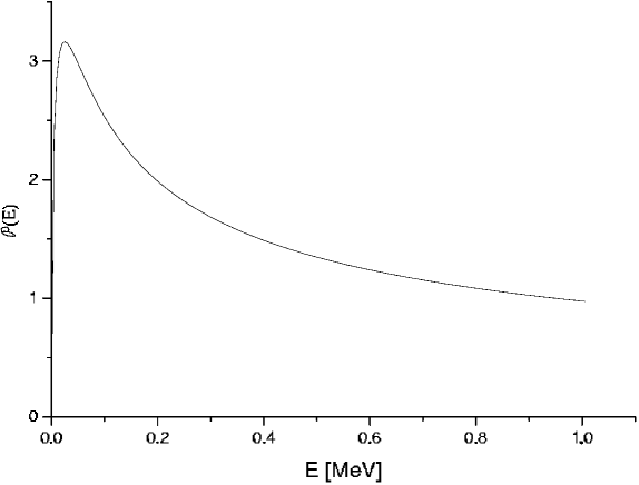
Figure 4: The function $\frac{{\cal P}(E)}{A}$, Eq. (15), corresponding to the antibound state at energy $E_{0}$=-0.025 MeV of Fig. 3.

The conclusion of this discussion is that poles may have physical meaning only if the corresponding wavefunction is localized. As an illustration of a non-localized pole we show in Fig. 5 the wavefunction corresponding to the ”resonance” $0d_{3/2}$ of Table 1. This state is so wide that it may be considered part of the continuum background since in a region surrounding the nuclear core its value is very small. As for the antibound state discussed previously the wavefunction increases with distance, but the difference with that case is that now the increase is huge even at a rather short distance. This state cannot be expected to have any physical significance. Yet we will include it in the generalized Berggren basis. In fact, one of the reasons why we apply in our calculations high presicion methods tv2 is to avoid numerical errors which would otherwise appear when states with large imaginary parts have to be considered.

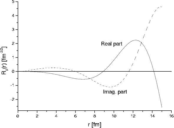
Figure 5: Radial wavefunction $R_{0d_{3/2}}(r)$ corresponding to the ”resonance” of Table 1. Notice the large values of the wavefunction here in comparisson with those in Fig. 3.

A state that will be fundamental to build the low lying spectrum of ¹¹Li is the Gamow pole $0p_{1/2}$ and, therefore, we show the corresponding wavefunction in Fig. 6. The imaginary part of the energy is in this case not very small in comparisson to the corresponding real part. Yet the wavefunction shows clear localization features. This state can be considered a resonance.

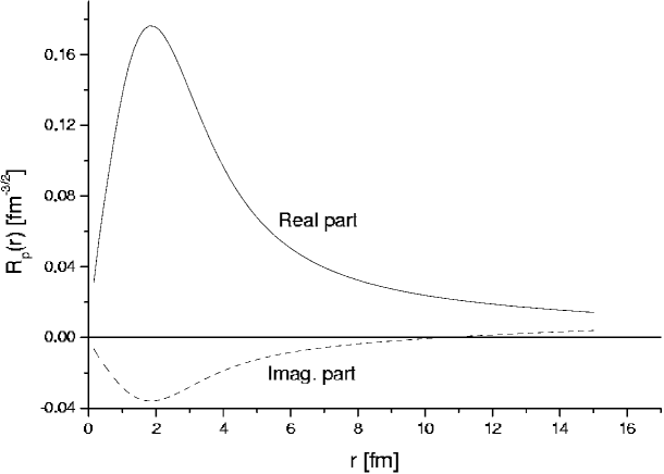
Figure 6: Radial wavefunction $R_{0p_{1/2}}(r)$ corresponding to the single-particle state in Table 1.

One does not need to use the same integration contour for all the single-particle states, since within the Berggren metric basis states are independent of each other. It is therefore convenient to use in each case a contour adapted to the position of the poles. In our case only for the antibound state it is necessary to have a contour that lies outside the fourth quadrant in the complex energy plane, as the one in Fig. 2. For the other partial waves corresponding to the poles of Table 1 we will use a contour as the one in Fig. 1. Moreover, in each segment $V_{i}-V_{i-1}$ (with $i>0$ and $V_{0}=(0,0)$) we choose different number of points according to how near a pole is to the segment. The values of the vertices $V_{i}$ and the number of points $N_{i}$ between adjacent vertices defining our Berggren basis is given in Table 2. The value of $N_{i}$ is the smallest number of Gaussian points which provides a convergence of the results of at least 5 digits in the energies and at least 4 digits in the wavefunctions.

Table 2: Vertices $V_{i}$ (in MeV) in the integration contours of Fig. 1 corresponding to all partial waves with values of $(l,j)$ as those in the states of Table 1 except for the partial wave $s_{1/2}$ for which the contour shown in Fig. 2 was used. $N_{i}$ is the number of Gaussian integration points in the segment between the vertices $V_{i}$ and $V_{i-1}$. The point $V_{0}$ (not shown in the Table neither in the Figures) is the origin, i. e. $V_{0}=(0,0)$. The energy cut-off point is $(c,0)$ = 10 MeV and the number of Gaussian points between the last vertex and the cutt-off point $(c,0)$ is 4 in all cases.

partial wave	$V_{1}$	$N_{1}$	$V_{2}$	$N_{2}$	$V_{3}$	$N_{3}$	$V_{4}$	$N_{4}$	$V_{5}$	$N_{5}$
$s_{1/2}$	(-0.025,0.1)	10	(-0.050,0)	10	(0,-0.7)	20	(3,-0.7)	6	(3,0)	2
$p_{3/2}$	(0,0)	2	(0,-0.7)	4	(3,-0.7)	4	(3,0)	4	——	—
$p_{1/2}$	(0,0)	2	(0,-0.7)	6	(3,-0.7)	10	(3,0)	6	——	—
$d_{5/2}$	(3.5,0)	4	(3.5,-3)	4	(5,-3)	4	(5,0)	4	——	—
$d_{3/2}$	(5,0)	4	(5,-10.7)	4	(8,-10.7)	4	(8,0)	4	——	—

The valence poles plus the scattering states thus defined constitute our generalized single-particle Berggren basis.

The two-particle basis is built from the single-particle states as usually. To evaluate the two-body energies and corresponding wavefunctions one has to solve the dispersion relation (9). To determine the strength $G_{\alpha}$ we will use the standard procedure of adjusting its value to fit the lowest energy of the two-particle state carrying angular momentum $\lambda_{\alpha}$ (and parity $(-1)^{\lambda_{\alpha}}$, since the force is separable ).

The only two-neutron positive-parity state for which there is any experimental data in ¹¹Li is the ground state, i. e. $\lambda_{\alpha}$=0 (although due to the presence of the proton the real spin of ¹¹Li(g.s.) is $3/2^{-}$). The corresponding experimental energy is $\omega_{n_{\alpha}=1,\lambda_{\alpha}=0}\approx$-0.295 MeV gar .

The short range and attractive character of the residual nuclear interaction causes the lowest $0^{+}$ state to lie below the lowest two-particle configuration. Therefore the vertex $V_{2}=(a,0)$ in Fig. 2 has to fulfill the condition $\omega_{0^{+}_{1}}<2a$. This restricts the position of the vertex $V_{2}$ to the range $-0.1MeV<a<-0.025MeV$. As seen in Table 2 we use $V_{2}=(-0.050,0)$ MeV which is very close to the energy of the antibound state. This is not an optimal situation since close to a pole the scattering waves increase rapidly as the energy approaches the pole. In fact, one of the advantages of using the representation (5) for the Dirac delta function is to avoid the numerical difficulties that one encounters when integrating on the real energy axis in the presence of very narrow resonances. These difficulties can be overcome by choosing an integration countour lying far enough from the resonance energy shec . In our case the contour has to be near the pole and therefore we had to use many integrations points around the antibound state. This explains the relatively large values of $N_{1}$, $N_{2}$ and $N_{3}$ corresponding to the partial wave $s_{1/2}$ in Table 2.

Another undesirable feature of this situation is that the two-particle configurations corresponding to the scattering states may acquire values which are very large (according to Eq. (12)) and therefore unfamiliar. But this is not a problem in itself, since the wavefunction components in the complex energy plane depends upon the contour that one uses. It is worthwhile to point out again that the results have physical meaning only when evaluating quantities defined on the real energy axis, as for instance the energies of bound states or the angular momentum content of the two-particle wavefunctions of those bound states. The ground state of ¹¹Li lies at about -295 keV, as mentioned above, and the angular momentum content is about 60 % $s$-states and 40 % $p$-states, although some small components of other angular momenta are not excluded gar .

Notice that for bound states the angular momentum content $A_{l}$ does not depend upon the contour because it is a sum over all basis states. Thus, for states with angular momentum $\lambda_{\alpha}$ = 0 it is

$$A_{l}=\sum_{nn^{\prime}l^{\prime}\not=lj}X(nl^{\prime}j,n^{\prime}l^{\prime}j;\alpha)^{2}$$ (16)

which is a real number if the state $\alpha$ is bound and complex otherwise since the real energy axis is excluded as a contour to describe complex states. This also implies that $A_{l}$ (as well as all physical quantities corresponding to ”resonances” which are not isolated) may depend upon the contour if this contour defines a Berggren space which does not fully contain the ”resonance”. However, due to the normalization of the state it is $\sum_{l}A_{l}=1$ in all cases.

The imaginary part of $A_{l}$ may give a measure of how significant (isolated) is the complex state. If $|Im(A_{l})|$ is large then the state may be considered a part of the two-particle continuum background. Again here, it is not very clear what is meant by ”large” and it would be more convenient to answer this question by looking at the localization of the corresponding wavefunction, as we will do below.

The property that $A_{l}$ for bound states do not depend upon the contour has been used by us as an important test for checking our computer codes.

The energy of ¹¹Li(gs) will be fitted to adjust the strength $G_{\alpha}$ of the separable interaction. Therefore it is $G_{\alpha}$ which should remain the same and a real number (since the Hamiltonian is Hermitian) as one changes the contour.

Using for the field (11) the parameters $f_{0}$=10, $R^{\prime}$=4.5 fm and $a^{\prime}$=1.5 fm we evaluated within the generalized Berggren basis defined above the strength from Eq. (9) to obtain the value $G_{0}$=0.1659 MeV. Using as a contour the real energy axis we obtained the same value, confirming the formalism as well as the precision of our computer codes.

The dispersion relation has as many solutions as the dimension of the two-particle basis. The overwhelming majority of these solutions form part of the continuum background. These continuum states are easy to recognize because they feel the interaction very weakly and therefore they lie very close to their zeroth order energy, i. e. they are ordered according to the lines defining the contour. For illustrations of this feature see Ref. cxsm . The physically meaningful states are localized and, therefore, one expects that the main wavefunction configurations of the relevant two-particle states should correspond to bound states or resonances. One indeed finds this feature in the main wavefunction components of the ground state (i. e. $0^{+}_{1}$) at -0.295 MeV and in a state at (0.274,-0.247) MeV ($0^{+}_{2}$) which may be a resonance. The largest of those components are

$$|0^{+}_{1}>=(1.79,0)|(1s_{1/2})^{2}>+(0.15,1.02)|(1s_{1/2}c_{1})>+(0.03,0.98)|(1s_{1/2}c_{2})>$$

$$|0^{+}_{2}>=(0.70,0.12)|(0p_{1/2})^{2}>+(-0.50,-0.08)|(0p_{1/2}c_{3})>+(0.36,-0.15)|(0p_{1/2}c_{4})>$$

where $c_{i}$ are states belonging to the continuum contour, i. e. they are scattering waves with angular momenta $(l,j)$ and energies $\epsilon_{i}$ (in MeV) given by

$$|c_{1}>=|l=0,j=1/2,\epsilon_{1}=(-0.048,-0.031)>;~{}~{}|c_{2}>=|l=0,j=1/2,\epsilon_{2}=(-0.046,-0.056)>$$

$$|c_{3}>=|l=1,j=1/2,\epsilon_{3}=(0,-0.266)>;~{}~{}|c_{4}>=|l=1,j=1/2,\epsilon_{4}=(0,-0.119)>$$

These continuum states are important in the description of our relevant $0^{+}$ levels because the zeroth order energies of the corresponding two-particle basis states are very close to the correlated energies. However, the CXSM wavefunction components depend upon the contour one chooses and, therefore, they have physical meaning only if the contour coincides with the real energy axis, as in the continuum shell-model. This feature is valid even if the state is bound, although in this case the wavefunction itself does not depend upon the contour and it has the normal physical meaning of quantum mechanics, as we wil see below.

Since the components of the CXSM wavefunction are not well defined quantities it may seem unreasonable to probe features like localization by analysing such components, as we did above. However we have found that physically relevant states always have wavefunctions with main components consisting of bound or resonant single-particle states, independently of the contour one chooses. In our case, the quantity which has a physical (i. e. quantum mechanical) significance is the angular momentum content $A_{l}$, Eq. (16). We found that for the ground state $A_{l}$ is, in percentage, 49 % s-states, 47 % p-states and 4 % d-states, in agreement with experiment.

Although for bound states $A_{l}$ is real its components may be complex, contour dependent and with very large absolute values. For instance, in ¹¹Li(gs) the contribution of the pole-pole component $|(1s_{1/2})^{2}>$ is (3.218,0.004), while the pole-continuum components $|1s_{1/2}c_{i}>$, where $c_{i}$ is an s-wave on the contour, add up to (-8.473,-0.009) and the continuum-continuum components $|c_{i}c_{j}>$ to (5.746,0.005). The corresponding values for the p-waves is (0.598,-0.202) for the pole-pole component $|(1p_{1/2})^{2}>$, (-0.146,0.218) for the pole-continuum components $|1p_{1/2}c_{i}>$ and (0.001,-0.016) for the continuum-continuum components. The $p_{3/2}$, $d_{3/2}$ and $d_{5/2}$ contribution adds up to a total of (0.060,0). The total sum are the values 0.49 for the s-waves, 0.47 for the p-waves and 0.04 for the d-waves, as quoted above. That is, the total sum is real and represents a probability while the partial components have no meaning and are contour dependent. Notice that this is valid even for the pole-pole component, since its value is proportional to the wavefunction amplitude $X$ which depends upon the contour through the normalization constant (see Eq. (12)).

In a calculation performed on the real energy axis there is neither pole-pole nor pole-continuum contributions (since there is no bound single-particle state in this case) and all partial contributions are continuum-continuum components that are probabilities, i. e. they are real, positive and less than or equal to unity. These values coincide with the percentages of $A_{l}$ given above, once again checking the reliability of our codes.

For the $0^{+}_{2}$ state all partial contributions to $A_{l}$ are complex although they have to add to unity due to the normalization of the CXSM wavefunction. One thus obtains that $A_{l}$ is (13,-10) % s-states and (87,10) % p-states, indicating that this ”resonance” is mainly built upon the $0p_{1/2}$ single-particle resonance.

It is interesting to see how the mixing among the various components of the angular momentum content evolves as the strength of the interaction increases from the zeroth order value where the states are indeed given by the poles, i. e. for $G=0$ it is 100% s-states for $0^{+}_{1}$ and 100% p-states for $0^{+}_{2}$. In Table 3 we present the evolution of these values, as well as the energies of the states, as a function of the strength $G$.

Table 3: Energies E and angular momentum content $A_{l}$, Eq. (16), for the angular momenta $l=0,1$ and $2$ ($s,p$ and $d$), corresponding to the states $0^{+}_{1}$ and $0^{+}_{2}$ in ¹¹Li as a function of the interaction strength $G$. The values of E and G are in Mev while $A_{l}$ is $\times$ 100. The strength fitting the available experimental data is $G_{0}$=0.1659 MeV.

	$0^{+}_{1}$				$0^{+}_{2}$
G	E	s	p	d	E	s	p	d
0.01	-0.061	100	0	0	(0.466,-0.117)	0	(100,0)	0
0.05	-0.091	100	0	0	(0.388,-0.089)	(-4,0)	(104,0)	0
0.09	-0.092	100	0	0	(0.292,-0.144)	(-14,-12)	(114,12)	0
0.13	-0.102	99	1	0	(0.261,-0.224)	(14,-9)	(86,9)	0
0.17	-0.328	48	47	5	(0.271,-0.276)	(17,-4)	(83,4)	0

Looking at the imaginary values of these quantities as well as at the energy of the predicted $0^{+}_{2}$ state (i. e. (0.274,-0.247) MeV), which is large, one may doubt whether this state is indeed a resonance and therefore whether it could be detected experimentally. To decide upon this we will analyse its localization properties. But first we have to learn which are the features that determine such localization in this weakly bound nucleus. This can be done by studing the two-particle wavefunction of the bound ground state. This would help us to decide whether the state $0^{+}_{2}$ is indeed a resonance by comparing the properties of its wavefunction with those of the ground state. A convenient way of doing this is by exploiting the clustering features of the ground state wavefunction in the singlet (S=0) component jan83 . We will call $S(r)$ this singlet part of the wavefunction. Its expression can be found in Ref. jan83 .

Due to the two-neutron clustering one can recognize whether the center of mass of the two-neutron system remains inside the nuclear core by analysing $S(r)$ in some direction, for instance in the x-direction. That is we will choose $r=r_{1}=r_{2}$, where $\vec{r}_{i}=(r_{i},\theta_{i},\phi_{i})$ is the coordinate of the particle $i$ with $\theta_{i}=\pi/2,\phi_{i}=0$. Notice that this direction is irrelevant since the system is spherically symmetric.

In Fig. 7 we show the function $S(r)$ corresponding to the ground state of ¹¹Li. One sees that inside the nucleus the wavefunction of the two valence particles is highest and the corresponding imaginary part smallest, indicating that there is a localization. Since this is the quantum mechanical wavefunction corresponding to the bound system, its value should not only be independent of the contour but also it should represent a probability amplitude. Therefore the small imaginary part that appears at long distance has to be considered a limitation of the calculation. One also sees that this wavefunction extends far outside the nucleus, as expected since this is the feature that causes the halo. Yet, one may think that the imaginary part as well as the large value of the real part at large distances is an effect of the diverging character of the complex wavefunctions in the generalized Berggren basis. To be sure that this is not the case, and considering that this wavefunction has a physical meaning, we calculated it again but using the real energy axis as a representation. As seen in the Figure, we found that the wavefunction thus calculated is virtually the same as the one using the generalized Berggren representation. As with the imaginary part, there are small differences at large distances, and this has to be attributed to computational limitations that makes it difficult to treat exactly the diverging character of the single-particle states.

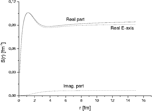
Figure 7: Two-particle radial wavefunction S(r) corresponding to the singlet component of the ground state of ¹¹Li evaluated by using the generalized Berggren representation. The dashed line is the same wavefunction but using as a representation the real energy axis, i. e. calculated within the Continuum Shell Model framework.

As a final comment, it has to be noted that although the two-particle wavefunction extends far in space (a feature which is known, see e. g. Fig. 1 of Ref. be ), the mean square radius of the nucleus is not excessively large since this quantity is strongly influenced by the particles in the core, including the three protons be . The extension of the wavefunction corresponding to the valence particles provides a tiny contribution to the total wavefunction of the nucleus, which is the reason why the density of the halo is low.

We are now in a position to analyse the wavefunction of the $0^{+}_{2}$ state. We thus plotted in Fig. 8 the singlet function S(r) for this state. We see that now the wavefunction does not show any localization feature inside the nucleus. Perhaps even worse, the imaginary part is very large, thus providing a large imaginary part of the ”probability” if it would be assigned a quantum mechanical meaning. This state is not a resonance and therefore it is not surprising that it has not been observed.

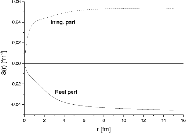
Figure 8: Two-particle radial wavefunction S(r) corresponding to the singlet component of the state ¹¹Li($0^{+}_{2}$) evaluated by using the generalized Berggren representation.

The narrowest $0^{+}_{2}$ state in Table 3 corresponds to G=0.05 MeV. One may thus learn from this case whether its small imaginary part of the energy implies that it is localized. We thus plotted in Fig. 9 the corresponding function S(r). One sees that something very strange happens. While the real part of the wavefunction shows localization the imaginary part does not. Again, the criterion of defining a resonance according to its localization features shows that neither this is a physically meaningful state. Yet, it is remarkable that as $G$ increases this state first becomes narrower and then, just after $G$=0.05 MeV in the Table, its width increases rather fast. This indicates that at this value of $G$ there is a mechanism that moves the state down in the complex energy plane. To examine this feature we show in Table 4 the dependence of the angular momentum content for each partial wave upon $G$. We show only the $s-$ and $p-$components since the other angular momenta play no role here. One sees in the Table that the mixing between these components is not as strong as the mixing between the pole-pole $|(1p_{1/2})^{2}>$ component and the pole-continuum components. It is also conspicuous that the continuum-continuum $l=1$ partial waves has virtually no influence. One therefore can conclude that the reason why the state does not become narrower as the interaction increases is that the coupling of the single-particle resonance to the continuum becomes stronger with an stronger interaction and, as a result, the two-particle state is itself pushed towards the continuum. At no value of $G$ the two-particle system in the $0^{+}_{2}$ complex state is trapped by the interaction inside the nucleus and the state never becomes a resonance.

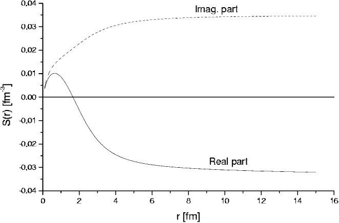
Figure 9: Two-particle radial wavefunction S(r) corresponding to the singlet component of the state ¹¹Li($0^{+}_{2}$) evaluated by using the generalized Berggren representation with a G=0.05 MeV interaction.

Table 4: Pole-pole (PP), pole-continuum (PC) and continuum-continuum (CC) contributions to the $s$ and $p$ angular momentum content $A_{l}$ corresponding to the state $0^{+}_{2}$ in ¹¹Li as a function of the interaction strength $G$. The values of G are in Mev while $A_{l}$ is $\times$ 100. The strength fitting the available experimental data is $G_{0}$=0.1659 MeV.

	$s-content$			$p-content$
G	PP	PC	CC	PP	PC	CC
0.01	0	0	0	(100,0)	0	0
0.05	(2,0)	(-4,5)	(-2,-5)	(104,2)	(0,-2)	0
0.09	(3,14)	(-31,-4)	(14,-22)	(101,20)	(13,-8)	0
0.13	(-8,-3)	(8,-17)	(14,11)	(36,30)	(50,-21)	0
0.17	(-6,-4)	(12,-16)	(11,16)	(39,20)	(44,-16)	0

Finally, it is interesting to analyse a $1^{-}$ state which was reported to be found at about 1.3 MeV and a width of about 0.75 MeV in a ${}^{11}Li+p$ experiment kor97 . From Table 1 one sees that this state lies too low to be a particle-hole excitation, since the lowest configuration of this type is $|1s_{1/2}0p_{3/2}^{-1}>$ at an energy of 4.5 MeV, and it lies too high to be a particle-particle state, since the lowest two-particle configuration is $|1s_{1/2}0p_{1/2}>$ at an energy of 0.215 MeV. Therefore we did not find any reasonable G value, even assuming a repulsive force (i. e. G real and negative) that could provide this state within our shell-model approach.

III.2 The nucleus ⁷⁰Ca

We have seen in the previous Subsection that in ¹¹Li(gs) the halo is induced by the extension of the wavefunctions corresponding to the valence single-particle states. This, in turn, is due to the lack of a barrier that would hold the particles tightly bound to the core. It is a delicate balance, since without the pairing interaction acting upon the valence particles the nucleus would not be bound, i. e. the ground state wavefunction would not be localized. One may therefore wonder whether valence single-particle states larger than $l=1$ would still induce halos. With this aim in mind we tried to find such a case by following the trend of single-particle states in a relativistic mean field calculation. We thus found that the nucleus ⁷²Ca (corresponding to the core Z=20, N=50) fulfills the conditions that we look for, since the valence single-particle states are again an antibound $2s_{1/2}$ shell but now the next shell is $2d_{5/2}$. In order to simulate the order of the single particle states given by the relativistic calculations we used a Wood-Saxon potential defined by $a$ = 0.67 fm, $r_{0}$ = 1.27 fm, $V_{0}$ = 39 MeV and $V_{so}$ = 22 MeV. The corresponding single-particle states are shown in Table 5. One sees that the antibound state as well as the first excited state lie near the energy threshold, as in the previous case. Even the wavefunction of the antibound state is similar to the one in ¹⁰Li, as expected. However, since now the first excited state carries a higher angular momentum as compared with the previous case, one would expect that the corresponding wavefunction would be too much localized, thus hindering the formation of the halo. As seen in Fig. 10 this is not the case since the wavefunction extends much beyond the standard value of the nuclear radius in ⁷¹Ca, i. e. $R$=5.18 fm.

Table 5: Valence single-particle states used in the calculation of the two-neutron states in ⁷²Ca. The energy $E_{n}$ and the wave number $k_{n}$ are related as in Eq 2. The $k_{n}-$value corresponding to the state $2s_{1/2}$ shows that this is an antibound state.

State	$E_{n}$ (MeV)	$k_{n}$ (fm-1)
$2s_{1/2}$	(-0.056,0)	(0,-0.051)
$1d_{5/2}$	(0.488,-0.053)	(0.153,-0.008)
$1d_{3/2}$	(2.089,-1.545)	(0.334,-0.110)
$0g_{7/2}$	(6.772,-0.748)	(0.568,-0.031)
$0h_{11/2}$	(5.386,-0.106)	(0.506,-0.005)

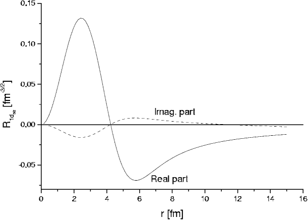
Figure 10: Radial wavefunction $R_{1d_{5/2}}(r)$ corresponding to the single-particle state in Table 5.

There is another important difference between the single-particle states in Tables 1 and 5, namely the appearance of the narrow high spin resonance $0h_{11/2}$. This may induce a high-lying localized two-particle resonance.

To probe the differences, if any, between ¹¹Li and ⁷²Ca we proceeded as in the previous subsection and solved the generalized CXSM in this case by using the separable interaction provided by the field $f$ of Ref. ant . As already reported in that reference, we thus found that the ground state two-particle wavefunction has the same features as the corresponding one in ¹¹Li.

There is also a second $0^{+}$ state lying at (0.550,-0.350) MeV. which in Ref. ant was considered to be a likely resonance. We have now the possibility to examine whether this is the case by looking at the wavefunction $S(r)$. The notable peculiarity of this wavefunction is that it looks very similar to the corresponding one in ¹¹Li, as can be seen by comparing Figs. 8 and 11. It thus seems that the nuclei ¹¹Li and ⁷²Ca are both halo nuclei although the valence wavefunctions correspond to different number of nodes and even orbital angular momenta. This shows, once more, that the characteristic determining the formation of halos is the extension of the valence wavefunctions in space, and this may happens even if the valence particles move in high angular momentum orbits.

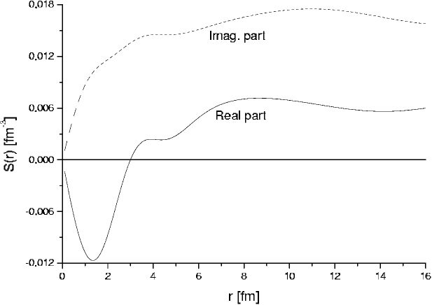
Figure 11: Two-particle radial wavefunction S(r) corresponding to the singlet component of the state ⁷²Ca($0^{+}_{2}$) evaluated by using the generalized Berggren representation.

We have also investigated whether it appears a narrow two-particle resonance as a result of the coupling of the particles in the single-particle state $0h_{11/2}$. This we did not observe by using the strength $G_{0}$ that provides the bound ground state of ⁷²Ca. We then decided to follow the trajectory in the complex energy plane of the state $|0h^{2}_{11/2}>$ as $G$ increases from its zeroth order value. As in Ref. cxsm we found that this state indeed becomes narrower as $G$ increases to a certain point, but afterwards the coupling of one of the particles to the continuum increases the width of the resonance which eventually becomes itself part of the continuum background. We have already seen this feature above when analysing the state $0^{+}_{2}$ in ¹¹Li and it appears again in the halo nucleus ⁷²Ca as well as in the drip line nuclei analysed previously by us cxsm . This teory thus predicts that only if the pairing interation is relatively weak two-particle resonances would appear as the result of the coupling of the particles to high lying narrow single-particle resonances.

IV Summary and conclusions

In this paper we have presented a new formalism to evaluate microscopically two-particle resonances in halo nuclei by using a generalization of the complex shell model (CXSM) presented in Ref. cxsm . Since one of the elements inducing the formation of halos was found to be the appearance of antibound states lying close to the continuum threshold, this generalization consists in defining a contour in the complex energy plane which comprises the antibound states. That is, the antibound states and the Gamow states (i. e. states lying in the complex energy plane) are selected by appropiate contours in the complex energy plane. Terefore within this formalism bound states, antibound states, Gamow states and the continuum background are all basis single-particle states treated on the same footing. These states are poles of the corresponding single-particle Green function.

The contribution of the pole-pole, pole-continuum and continuum-continuum configurations in the two-particle systems can be easily analysed. The effects induced by antibound states and the continuum encircling the poles can be studied separately.

Given the rather unfamiliar characteristics of both the CXSM and the antibound states we have described in detail those characteristics. In particular, we have shown that the effects induced by antibound states lying close to threshold upon physically measurable quantities is exactly the same as those provides by bound states lying also close to threshold. In both cases the main feature is that the single-particle wavefunction extends far in space.

We have also analysed the properties that a many-particle state lying on the complex energy plane may have to be considered a ”resonance”, i. e. a measurable state appearing in the continuum part of the spectrum. We have thus found that the resonant wavefunction has to be localized within the nuclear system. In order to illustrate these features as well as to show the advantages of the formalism we evaluated two-particle states in the well known case of ¹¹Li as well as in the nucleus ⁷²Ca. We analysed the localization properties of the two-particle wavefunctions in these nuclei trying to find high lying resonances. However we did not find evidences that would indicate that such resonances exist in these cases.

Finally, we have found that the theory predicts that only if the two-body interation is relatively weak two-particle resonances would appear as the result of the coupling of the particles to high lying narrow single-particle resonances.

- (1) M. V. Zhukov, B. V. Danilin, D. V. Fedorov, J. M. Bang, I. J. Thompson and J. S. Vaagen, Phys. Report 231, 151 (1993).
- (2) E. Garrido, D. V. Fedorov and A. S. Jensen, Nucl. Phys. A700, 117 (2002).
- (3) Y. Suzuki, R. G. Lovas, K. Yabana and K. Varga, Structure and Reactions of Light Exotic Nuclei, Taylor and Francis, London, 2003.
- (4) J. Okolowicz et. al., Phys. Rep. 374, 271 (2003) and references therein.
- (5) R. Id Betan, R. J. Liotta, N. Sandulescu and T. Vertse, Phys. Rev. Lett. 89, 042051 (2002)
- (6) N. Michel, W. Nazarewicz, M. Ploszajczak and K. Bennaceur, Phys. Rev. Lett. 89, 042052 (2002).
- (7) R. Id Betan, R. J. Liotta, N. Sandulescu and T. Vertse, Phys. Rev. C 67, 014322 (2003).
- (8) R. Id Betan, R. J. Liotta, N. Sandulescu and T. Vertse, Phys. Lett. 584B, 48 (2004).
- (9) G. Gamow, Z. Phys. 51, 204 (1928).
- (10) R. Peierls anf P. Kapur, Proc. Roy. Soc. A166, 277 (1938).
- (11) R. G. Newton, Scattering theory of waves and particles (McGraw-Hill, NY, 1966) p368.
- (12) B. Gyarmati and T. Vertse, Nucl. Phys. A160, 523 (1971).
- (13) T. Berggren, Nucl. Phys. A 109, 265 (1968).
- (14) R. J. Liotta, E. Maglione, N. Sandulescu and T. Vertse, Phys. Lett. 367B, 1 (1996).
- (15) T. Vertse, P. Curutchet and R. J. Liotta, ”Resonances, the unifying route towards the formulation of dynamical processes”, Proceedings, Lertorpet, Sweden, 1987. Eds. E. Brändas and N. Elander, Lecture Notes in Physics Vol. 325, Springer Verlag, Berlin, 1989.
- (16) G. Breit and E. P. Wigner, Phys. Rev. 49, 519 (1936).
- (17) T. Vetse, R.J. Liotta, and E. Maglione, Nucl. Phys. A584, 13 (1995).
- (18) T. Berggren, Phys. Lett. B 73, 389 (1978).
- (19) J. Humble and L. Rosenfeld, Nucl. Phys. A26, 529 (1961).
- (20) V. I. Kukulin, V. M. Krasnopolsky and J. Horacek, Theory of resonances, (Kluver, Boston, 1989), p. 151.
- (21) G. F. Bertsch and H. Esbensen, Ann. of Phys. 209, 327 (1991).
- (22) H. Esbensen, G. F. Bertsch and K. Hencken, Phys. Rev. C 56, 3054 (1997).
- (23) A. Bianchini, R.J. Liotta, and N. Sandulescu, Phys. Rev. C63, 024610 (2001).
- (24) T. Vertse, P. Curutchet, R. J. Liotta, and J. Bang, Acta Phys. Hungarica, 65, 305 (1989).
- (25) T. Berggren, and P. Lind, Phys. Rev. C 47, 768 (1993).
- (26) L. Gr. Ixaru, Numerical Methods for Differential Equations, (Reidel, Dordrecht 1984); L. Gr. Ixaru, M. Rizea and T. Vertse, Comput. Phys. Commun. 85, 217 (1995).
- (27) I. J. Thompson and M. V. Zhukov, Phys. Rev. C 49, 1904 (1994).
- (28) H. G. Bohlen et. al., Nucl. Phys. A616, 254c (1997).
- (29) A. B. Migdal, Yad. Fiz. 16, 427 (1972) [Sov. J. Nucl. Phys 16 238 (1972)].
- (30) R. G. Lovas, R. J. Liotta, A. Insolia, K. Varga, and D. S. Delion, Phys. Rep. 294, 265 (1998).
- (31) T. Vertse, A. T. Kruppa, R. J. Liotta, W. Nazarewicz, N. Sandulescu and T. R. Werner, Phys. Rev. C 57, 3089 (1998).
- (32) F. Janouch and R. J. Liotta, Phys. Rev. C 27, 896 (1983).
- (33) A. A. Korsheninnikov et. al., Phys. Rev. Lett. 78, 2317 (1997).