The Nuclear matter stability in a non-local chiral quark model

Abstract

We study the stability of the nuclear matter in a non-local Nambu-Jona-Lasinio model. We work out the equation of state in a relativistic Faddeev approach where we take into account the internal structure of nucleon. We show that the binding energy saturates when the nucleon as a composite particle made of quarks is incorporated. After truncation of the two-body channels to the scalar and axial-vector diquarks, a relativistic Faddeev equation for nucleon bound states in medium is solved in the covariant diquark-quark picture. We investigate the nucleon properties in the nuclear medium such as the role of diquarks within the nucleon and the in-medium modification of the nucleon mass and size.

I Introduction

Chiral type models such as the NJL model have been successful in explaining the low energy physics of mesons and nucleons in vacuum utilizing the concept of the spontaneous chiral symmetry breaking njl . Application of the model to low density, however, has posed serious problems like the absence of saturation sa-1 ; sa-1-1 ; sa-2 ; under2 . This is in contrast to non-chiral models like the Walecka model sa-3 which has been phenomenologically successful in describing the nuclear matter ground state in the mean field approximation.

In chiral models with a Mexican hat potential, the nuclear medium moves the minimum of the vacuum effective potential towards smaller values. This implies a smaller curvature, i.e. the scalar sigma mass decreases. Consequently, the attraction between nucleons due to sigma meson exchange increases. This effect may destroy the stability of nuclear matter. On the contrary, in non-chiral models e.g. the Walecka type model, where the potential is simpler, a stable nuclear matter can be found.

At the nuclear matter saturation point the Fermi momentum $k_{f}$ and the pion mass $m_{\pi}$ are of comparable scale ($k_{f}\simeq 262MeV\simeq 2m_{\pi}$). Therefore, chiral dynamics may play an important role in a nuclear matter saturation mechanism. Chiral symmetry is an approximate symmetry for quarks which is not necessarily translated into a symmetry for nucleon degrees of freedom. Furthermore, the delta-nucleon mass splitting $\Delta=293$ MeV is also comparable to the Fermi momentum $k_{f}$ at nuclear matter saturation. It has been shown that the main mechanism behind the delta-nucleon mass splitting stems from the fact that the delta and the nucleon have different internal quark structure delta1 ; njln3 . Therefore one may naturally be led to ask if the internal structure of nucleon is important in order to describe the empirical nuclear matter ground state. Quark degrees of freedom have also been important in order to describe deep-inelastic scattering at momentum transfers of several GeV and the EMC effect p1 ; sa-4 ; fad-new .

Moreover, at the moment a direct calculation of the many nucleons system based on QCD itself is not feasible. Therefore, effective quark theories are the best tools to develop a microscopic understanding of a single nucleon together with nuclear and quark matter and their phase structure in a unified framework.

It has been shown that a non-local covariant extension of the NJL model inspired by the instanton liquid model non1 can lead to quark confinement for acceptable values of the parameters pb . There are other advantages of the non-local version of the model over the local NJL model, for example: the constituent quark mass is momentum-dependent, as also found in lattice calculation lat-m . The regulator makes the theory finite to all orders in the loop expansion and leads to small next-to-leading order corrections pb-2 . This model has been phenomenologically very successful to describe mesons pb ; pb-2 ; a1 and baryons a3 ; me1 in vacuum. More applications can be found in Refs. a2 ; non-s2 . Here, we employ this model to investigate the role of the internal dynamics of nucleon in a nuclear matter environment. We explicitly construct nucleon degrees of freedom by binding diquarks and quarks with relativistic Faddeev equations to describe nuclear matter. The relativistic Faddeev approach to describe the nucleon as a composite object has been very successful under2 ; njln1 ; fad-new ; njln3 ; o1 ; o2 ; me1 ; me2 .

Very recently Bentz and Thomas under2 have shown that local NJL models may lead to saturating nuclear matter when the quark confinement effect is incorporated to avoid unphysical thresholds. Although the idea is interesting, there may be some short-coming in their approach. Quark confinement in their prescription is incorporated by introducing an infrared cutoff in the model. This way quark confinement is permanent and there is no confinement-deconfinement transition in their model. In their hybrid approach, the nucleon is described as a relativistic bound state in the static approximation of a scalar diquark and quark. It has been already noticed that the attractive axial-vector diquark plays an important role in description of a single nucleon njln3 ; me1 . Therefore, in order to treat the internal structure of the nucleon and its modification in the medium adequately, we will take into account both the scalar and the axial-vector diquark channels and solve the Faddeev equation without invoking the static approximation.

We start by investigating the role of diquarks in the bound nucleon. The in-medium modification of the nucleon mass and the nucleon size will be calculated. We obtain the nuclear matter equation of state when nucleon is taken as a composite object made of diquark and quark.

This paper is organised as follows: In Sec. II we introduce the model, discuss its pionic sector and fix the parameters. In Sec. III we set up the description of the nucleon based on a diquark-quark picture in the relativistic Faddeev approach. In Sec. IV we consider nuclear matter with composite nucleons and present our numerical results. Finally, a summary and outlook is given in Sec. VI.

II Formalism and solution in the vacuum and quark matter

We consider a non-local NJL model Lagrangian in terms of quark degrees of freedom with $SU(2)_{f}\times SU(3)_{c}$ symmetry

$$\mathcal{L}=\bar{\psi}(i\partial\kern-4.49997pt/-m_{c})\psi+\frac{1}{2}g_{\pi}j_{\alpha}(x)j_{\alpha}(x),$$ (1)

where $m_{c}$ is the current quark mass of the $u$ and $d$ quarks. First, we restrict the interaction terms to four-quark interaction vertices in the quark-antiquark channels. We will add in section III the diquark channels in order to model the quark sub-structure of the nucleon in the medium. The current $j_{\alpha}(x)$ has the scalar ($0^{+},T=0$) and pseudoscalar ($0^{-},T=1$) components

$$j_{\alpha}(x)=\int d^{4}x_{1}d^{4}x_{3}F(x-x_{3})F(x_{1}-x)\overline{\psi}(x_{1})\Gamma_{\alpha}\psi(x_{3}),$$ (2)

with $\Gamma_{\alpha}=(1,i\gamma_{5}\vec{\tau})$. The ${\tau_{i}}$’s are flavour $SU(2)$ matrices with $\operatorname{tr}(\tau_{i}\tau_{j})=2\delta_{ij}$. Notice that there are different approaches asy ; non-bir to introduce non-locality into the interactions. We use the four-way separability of the non-local interaction which is also present in the instanton liquid model sep-i . This assumption considerably simplifies the calculation. Non-locality also emerges naturally in the presence of other gluonic field configurations within the QCD vacuum gluon and in models based on Schwinger-Dyson resummation techniques asy .

In the medium the repulsive vector mesons are important. For simplicity we add a local vector field interaction $-g_{v}(\overline{\psi}\gamma^{\mu}\psi)^{2}$ to the Lagrangian. Locality of this term is permissible as long as the interactions in Lagrangian are not fixed by some underlying theory through a Fierz transformation. Upon standard bosonization we obtain

$$\mathcal{L} = \int d^{4}x_{1}d^{4}x_{3}\overline{\psi}(x_{1})\Big{[}\left(i\partial\kern-4.49997pt/-m_{c}\right)\delta(x_{1}-x_{3})\delta(x_{3}-x)+F(x-x_{3})F(x_{1}-x)\left(\sigma(x)+\vec{\pi(x)}i\gamma_{5}\vec{\tau}\right)$$ (3)

$$- \gamma^{\mu}\omega_{\mu}(x)\delta(x_{1}-x_{3})\delta(x_{3}-x)\Big{]}\psi(x_{3})-\frac{1}{2g_{\pi}}[\sigma^{2}(x)+\pi^{2}(x)]+\frac{1}{4g_{v}}\omega_{\mu}(x)\omega^{\mu}(x).\$$

Lagrangians (1) and (3) are equivalent in the classical limit. The equations of motion for bosonic fields lead to

$$\left(\sigma(x),\vec{\pi}(x)\right) = g_{\pi}\int d^{4}x_{1}d^{4}x_{3}F(x-x_{3})F(x_{1}-x)\overline{\psi}(x_{1})\left(1,i\gamma_{5}\vec{\tau}\right)\psi(x_{3}),$$

$$\omega^{\mu}(x) = 2g_{v}\overline{\psi}(x)\gamma^{\mu}\psi(x).\$$ (4)

The Lagrangian (1) can be immediately recovered from the bosonized version Eq. (3) by substituting Eq. (4) into Eq. (3).

We define the Fourier transform of the form factor by

$$F(x-x_{i})=\int\frac{d^{4}p}{(2\pi)^{4}}e^{-i(x-x_{i})\cdot p}f(p).$$ (5)

The function $f(p)$ influences the momentum distribution of quarks in the non-perturbative vacuum and will be defined later. Next, we perform a mean field approximation by expanding the meson fields around their expectation values $\overline{\sigma}=\langle\sigma\rangle$, $\overline{\omega}^{0}=\langle\omega^{0}\rangle$ neglecting meson fluctuations. The mean values of the pion field and space components of the vector field vanish in vacuum and for a baryonic matter at rest due to symmetry. The mean field Lagrangian in momentum space can then be written as

$$\mathcal{L}=\overline{\psi}(p)\left(ip\kern-4.49997pt/-M(p)-\gamma^{0}\overline{\omega}_{0}\right)\psi(p)-\frac{\overline{\sigma}^{2}}{2g_{\pi}}+\frac{\overline{\omega}_{0}^{2}}{4g_{v}},$$ (6)

where the momentum-dependent quark mass and quark propagator are given by

$$M(p)=m_{c}+f^{2}(p)\overline{\sigma},$$ (7)

$$S^{-1}(p)=p\kern-4.49997pt/-M(p)-\gamma^{0}\overline{\omega}_{0}.\$$ (8)

We treat the quark fields at one-loop level and the meson fields at tree level. This approximation is consistent with the leading-order behaviour of the model in a $1/N_{c}$ expansion. Within this approximation the effective potential can be calculated:

$$\Omega=i\gamma_{q}\int\frac{d^{4}k}{(2\pi)^{4}}\ln\left(k^{2}-M^{2}(k)\right)+\frac{\overline{\sigma}^{2}}{2g_{\pi}}-\frac{\overline{\omega}_{0}^{2}}{4g_{v}},$$ (9)

where $\gamma_{q}=2N_{c}N_{f}$ is the degeneracy factor for quarks. A gap equation is obtained by requiring $\frac{\partial\Omega}{\partial\overline{\sigma}}=0$:

$$\overline{\sigma}=2g_{\pi}\gamma_{q}i\int\frac{d^{4}k}{(2\pi)^{4}}\frac{M(k)f^{2}(k)}{k^{2}-M^{2}(k)},$$ (10)

where the dynamical quark mass is given in Eq. (7).

Our model contains four parameters: the current quark mass $m_{c}$, the cutoff ($\Lambda$) hidden in the form factor $f(p)$ and the coupling constants $g_{\pi}$ , $g_{v}$. The vector field coupling $g_{v}$ is treated as a free parameter and will be adjusted in the medium. We first fix $g_{\pi}$ and $m_{c}$ for arbitrary values of $\Lambda$ by fitting the pion mass $m_{\pi}$ and the pion decay constant $f_{\pi}$ to their empirical values at zero baryon density. In this way, we can consider the entire parameter space of the model. The pion mass is given by the zero of the 1PI two-point function $\Pi_{\pi\pi}(q)$ for the pion which in random phase approximation has the following form

$$\Pi_{\pi\pi}(q)=\frac{1}{g_{\pi}}+i\operatorname{Tr}\int\frac{d^{4}k}{(2\pi)^{4}}f^{2}(k)\gamma_{5}\tau_{i}S(k)\gamma_{5}\tau_{i}S(q+k)f^{2}(q+k)=0,$$ (11)

where $q$ denotes the total momentum of the quark-antiquark pair. The pion decay constant $f_{\pi}$ is obtained from the coupling of the pion to the axial-vector current pb

$$f_{\pi} = \frac{ig_{\pi\bar{q}q}}{m_{\pi}^{2}}\int\frac{d^{4}p}{(2\pi)^{4}}\operatorname{Tr}[q\kern-4.49997pt/\gamma_{5}\frac{\tau_{a}}{2}(S(p_{-}))\gamma_{5}\tau_{a}(S(p_{+}))]f(p_{-})f(p_{+})$$ (12)

$$- \frac{g_{\pi}g_{\pi\bar{q}q}}{2m^{2}_{\pi}}\int\frac{d^{4}k}{(2\pi)^{4}}\operatorname{Tr}[S(k)]\int\frac{d^{4}p}{(2\pi)^{4}}\operatorname{Tr}[\tau^{a}\gamma_{5}f(p_{-})f(p_{+})S(p_{-})\gamma_{5}\tau_{a}S(p_{+})]$$

$$\times[f^{2}(k)\left(f^{2}(p_{+})+f^{2}(p_{-})\right)-f(p_{+})f(p_{-})f(k)\left(f(k+q)+f(k-q)\right)],\$$

where $g_{\pi\bar{q}q}$ is the pion-quark-antiquark coupling constant and related to the corresponding loop integral Eq. (11) by $g_{\pi\bar{q}q}^{-2}=(\frac{d\Pi_{\pi\pi}}{dq^{2}})|_{q^{2}=m^{2}_{\pi}}$. We define $p_{\pm}=p\pm\frac{1}{2}q$. Notice that due to non-locality the one-pion-to-vacuum matrix element gets an additional contribution. This extra term is very important to maintain the Gell-Mann-Oakes-Renner relation pb and makes a significant numerical contribution.

In our numerical treatment of the model, we evaluate loop-integrals like that in Eqs. (10,11,12) in Euclidean space. We choose for the form factor in Eq. (5) a Gaussian function in Euclidean space,

$$f(p_{E})=\exp(-p_{E}^{2}/\Lambda^{2}),$$ (13)

where $\Lambda$ is the cutoff of the theory. This choice respects Poincaré invariance and for certain values of the parameters it leads to the quark ”confinement” in the sense that the dressed quark propagator has no poles at positive $p^{2}$ in Minkowski space and consequently, quarks do not appear as asymptotic states. Quark ”confinement” can occur if the following relation is satisfied between the parameters of the model

$$\frac{\overline{\sigma}}{\sqrt{m^{2}_{c}+\Lambda^{2}}-m_{c}}>\frac{1}{2}\exp\left(-\frac{(\sqrt{m^{2}_{c}+\Lambda^{2}}+m_{c})^{2}}{2\Lambda^{2}}\right).$$ (14)

Notice that the quark propagator has many pairs of complex poles, both for confining and non-confining parameter sets which can be conceived as a remnant of the underlying confinement. Confinement in this model has direct consequence for the pion, but condition Eq. (14) is not derived by using any assumption about pions.

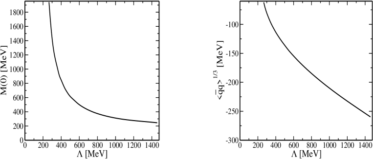
Figure 1: The zero-momentum constituent quark (left panel) and quark condensate (right panel) as a function of cutoff for fixed $f_{\pi}=93$ MeV and $m_{\pi}=140$ MeV when $m_{c}\neq 0$.

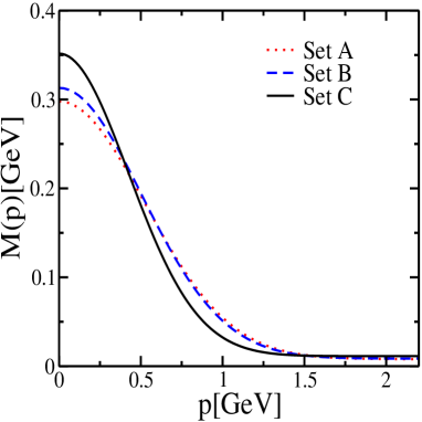
Figure 2: The constituent quark mass $M(p)$ as a function of momentum $p$ for the three parameter sets given in Table 1.

Table 1: The parameters $\Lambda$, $g_{\pi}$ and $m_{c}$ for the sets $A$, $B$ and $C$, fitted to $f_{\pi}=92.4$ MeV and $m_{\pi}=139.6$ MeV. The resulting values of the constituent quark mass $M(0)$ (in brackets we give the values for zero current quark mass) and the corresponding quark condensate for the different parameter sets are also given.

Parameter	set A	set B	set C
$\Lambda$ (MeV)	1046.8	1008.1	847.8
$g_{\pi}(\text{GeV}^{-2})$	31.6	35.2	55.80
$m_{c}$ (MeV)	7.9(0)	8.5(0)	11.13(0)
$M(0)$ (MeV)	297.9(250)	313(264.5)	351.6(300)
$-\langle\bar{q}q\rangle^{1/3}$ (MeV)	215(208)	212(205)	191(186)

Table 2: The first two sets of poles of the quark propagator $\pm M_{R}\pm iM_{I}$ in Minkowski space with $m_{c}\neq 0$ .

set A	set B	set C
$\pm 391$ MeV	$\pm 507\pm i55$ MeV	$\pm 408\pm i238$ MeV
$\pm 675$ MeV	$\pm 1530\pm i253$ MeV	$\pm 1575\pm i307$ MeV

The emergence of complex poles for quark propagators was also noticed in Schwinger-Dyson equation studies in QED and QCD sde-p ; sde-new ; sde-qe . It has been recently shown that baryons become more compact in the presence of imaginary poles in the quark propagator me1 . In another study it has been noticed that the mass-like singularities are located on the time axis if one removes the confining potential in QED in 2+1D, and the mass-like singularities move from the time axis to complex momenta if there is a confining potential sde-qe .

We refer to appendix for details of numerical evaluation of loop integrals as of Eq. (11). Solutions of the gap equation (10) are shown in Fig. 1. In the left panel the constituent mass at zero momentum $M(0)$ is shown as a function of the cutoff. It is obvious that for very small cutoff, there is no solution for the gap equation. On the right panel of Fig. 1, we show the corresponding values of the quark condensate. These values are within the limits extracted from QCD sum rules qcdsum and also lattice calculation lat-con . Notice that the trend of the model parameters in Fig. 1 is slightly different to that obtained in the local NJL model with a sharp cutoff bub1 . In contrast to the local NJL model, the dynamical quark mass Eq. (7) is momentum dependent (see Fig. 2) and follows a very similar trend to lattice simulations lat-m . Fig. 2 shows that at low virtualities the quark mass is close to the constituent mass while at large virtualities it approaches the current mass.

We analyse three sets of parameters, as indicated in Table 2. Set $A$ is called the non-confining parameter set since it does not contain imaginary poles of the quark propagator. Sets $B$ and $C$ lead to the quark ”confinement” in our convention with complex poles. We define the pole mass to be given through the equation

$$P_{pole}^{2}=M^{2}(P_{pole}),$$ (15)

where pole solutions are denoted $P_{pole}=\pm M_{R}\pm iM_{I}$. Equation (15) is a non-linear equation and can be solved numerically. The position of the quark poles are given in Table 2 where it is seen that for the confining sets the quark poles lie in the complex plane. In contrast to the local NJL model, a non-zero current quark mass of order $8.5$ MeV leads to an increase of about $48.5$ MeV in the zero-momentum dynamical quark mass (see Table 1 set B). It is also noted that the real part of the pole mass is bigger than the zero-momentum constituent quark mass $M(0)$ for both the confining and the non-confining sets, see Tables 1,2.

III Nucleon internal structure

In order to have a physically realistic description of matter at low density, one has to construct nucleons and nucleon matter from the quark degrees of freedom since quarks are confined at very low density. In this section, we take into account the quark structure of the nucleon in a diquark-quark picture. We first build up a single nucleon out of the quark degrees of freedom by solving the relativistic Faddeev equation, then (in the next section) we construct nuclear matter in a mean field approximation by means of these individual nucleons. In this way, any reference to the quarks will be naturally hidden in the nucleons.

In the vacuum baryons and diquarks have already been solved in this model by one of the authors me1 . Here, we shortly recapitulate the procedure to construct the nucleon as a diquark-quark bound state, more details can be found in me1 ; me2 .

In order to describe the nucleon as a bound state of a diquark and a quark, we firstly introduce diquarks in the model. We truncate the quark-quark interaction to the scalar $(0^{+},T=0,\overline{3})$ and the axial vector $(1^{+},T=1,\overline{3})$ colour antitriplet,

$$\mathcal{L}_{Is,a}=g_{s}\overline{J}_{s}(x)J_{s}(x)+g_{a}\overline{J}_{a}(x)J_{a}(x),$$ (16)

where the currents are defined

$$\overline{J}_{s}(x) = \int d^{4}x_{1}d^{4}x_{3}f(x-x_{3})f(x_{1}-x)\overline{\psi}(x_{1})\big{[}\gamma_{5}C\tau_{2}\beta^{A}\big{]}\overline{\psi}^{T}(x_{3}),$$

$$J_{s}(x) = \int d^{4}x_{2}d^{4}x_{4}f(x-x_{4})f(x_{2}-x)\psi^{T}(x_{2})\big{[}C^{-1}\gamma_{5}\tau_{2}\beta^{A}\big{]}\psi(x_{4}),$$

$$\overline{J}_{a}(x) = \int d^{4}x_{1}d^{4}x_{3}f(x-x_{3})f(x_{1}-x)\overline{\psi}(x_{1})\big{[}\gamma_{\mu}C\tau_{i}\tau_{2}\beta^{A}\big{]}\overline{\psi}^{T}(x_{3}),$$

$$J_{a}(x) = \int d^{4}x_{2}d^{4}x_{4}f(x-x_{4})f(x_{2}-x)\psi^{T}(x_{2})\big{[}C^{-1}\gamma^{\mu}\tau_{2}\tau_{i}\beta^{A}\big{]}\psi(x_{4}).\$$ (17)

The object $C=i\gamma_{2}\gamma_{5}$ is the charge conjugation matrix. The matrices $\beta^{A}=\sqrt{3/2}\lambda^{A}(A=2,5,7)$ project onto the colour $\overline{3}$ channel with normalisation $\operatorname{tr}(\beta^{A}\beta^{A^{\prime}})=3\delta^{AA^{\prime}}$. The couplings $g_{s}$ and $g_{a}$ specify the strength in the scalar and axial-vector diquark channels, respectively. We fix them by the empirical nucleon mass. The form factor in the diquark sector is assumed to be the same as in the meson sector.

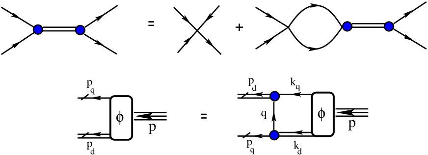
Figure 3: Top panel: A graphical representation of the Bethe-Salpeter equation for the $qq$ $T$-matrix in RPA approximation. The solid lines denote the dressed quark propagators Eq. (8) and double lines denote diquark propagators $D^{5},D^{\mu\nu}$. The filled circles denote the diquark vertices $\chi^{5},\chi^{\mu\nu}$. Down panel: The coupled effective Bethe-Salpeter equation for the nucleon vertex function $\phi$ is defined by amputating the external quark and diquark propagator from the wave function $\phi=S^{-1}D^{-1}\psi$.

In the ladder approximation the quark-quark $T$-matrix near the pole can be parametrised as me1 ; o2 ; me2

$$T(p_{1},p_{2};k_{1},k_{2})=T(p,k;q)\simeq\chi^{5}(p,q)D^{5}(q)\bar{\chi}^{5}(k,q)+\chi^{\mu}(p,q)D^{\mu\nu}(q)\bar{\chi}^{\nu}(k,q),$$ (18)

where $q=p_{1}+p_{2}=k_{1}+k_{2}$ is the total momentum of the quark-quark pair and $p,k$ are the relative momenta within the diquarks. The momentum-dependent scalar $\chi^{5}$, the axial $\chi^{\mu}$ diquark vertex functions, their adjoint functions $\bar{\chi}^{5}$ and $\bar{\chi}^{\mu}$ and the corresponding propagators $D^{5}(q)$ and $D^{\mu\nu}(q)$ can be obtained from solving the Bethe-Salpeter equation me1 for $qq$ scattering matrix shown in Fig. 3.

The scalar and the axial diquark masses $M_{ds}$ and $M_{da}$ are obtained as the position of the pole of the corresponding $T$-matrix in the scalar and axial-vector diquark channels, respectively.

With the diquark, the baryon can be constructed as a bound state of diquark-quark. We ignore the three-body irreducible graphs. Due to the separability of the two-body interaction in momentum-space, the relativistic Faddeev equation can be recast into an effective two-body Bethe-Salpeter type equation (pictorially shown also in Fig. 3)

$$\int\frac{d^{4}k}{(2\pi)^{4}}G^{-1}(p,k;P)\left(\begin{array}[]{c}\psi^{5}(k,P)\\ \psi^{\mu}(k,P)\end{array}\right)=0,$$ (19)

where the $G^{-1}(p,k;K)$ denotes the inverse of the full quark-diquark $4$-point function and contains the sum of the disconnected part and the one-quark exchange interaction kernel. After projecting the effective diquark-quark Bethe-Salpeter equation in the colour singlet and isospin $1/2$ channel, one finds

$$G^{-1} = (2\pi)^{4}\delta(p-k)S^{-1}(p_{q})\left(\begin{array}[]{cc}(D^{5}(p_{d}))^{-1}&0\\ 0&(D^{\nu\mu}(p_{d}))^{-1}\end{array}\right)$$ (22)

$$+ 3\left(\begin{array}[]{cc}\chi^{5}(p_{1},k_{d})S^{T}(q)\bar{\chi}^{5}(p_{2},p_{d})&-\sqrt{3}\chi^{\mu}(p_{1},k_{d})S^{T}(q)\bar{\chi}^{5}(p_{2},p_{d})\\ -\sqrt{3}\chi^{5}(p_{1},k_{d})S^{T}(q)\bar{\chi}^{\nu}(p_{2},p_{d})&-\chi^{\mu}(p_{1},k_{d})S^{T}(q)\bar{\chi}^{\nu}(p_{2},p_{d})\end{array}\right),\$$ (25)

where $\chi^{5}$ and $\chi^{\mu\nu}$ stand for the Dirac structures of the diquark vertices introduced in Eq. (18). The dressed quark propagator $S^{-1}(p)$ is defined in Eq. (8). The numerical coefficient in kernel of the Faddeev equation (25) comes from projecting the kernel to the physical baryon states (colour singlet and isospin half). We define the spectator quark momentum $p_{q}=\eta P+p$ and the diquark momentum $p_{d}=(1-\eta)P-p$, where $P$ is the total momenta in the diquark-quark pair and $\eta\in[0,1]$ is the Mandelstam parameter which parametrises the relative momenta within the quark-diquark system. The relative momentum of quarks in the diquarks vertices are defined as $p_{1}=p+k/2-(1-3\eta)P/2$ and $p_{2}=-k-p/2+(1-3\eta)P/2$, and the momentum of the exchanged quark is $q=-p-k+(1-2\eta)P$. We refer to Appendix for details of numerical methods involved in solving the Faddeev equation (25).

The parameters of the models $g_{\pi},m_{c}$ and $\Lambda$ are fixed by meson properties i.e. the pion mass and decay in vacuum as described in section II. We select parameter set C given in Table 1. Now the only unknown parameters are diquark couplings $g_{s}$ and $g_{a}$ and vector meson coupling $g_{v}$. The scalar and axial-vector diquark couplings are taken as independent parameters. One can find a line in parameter space of diquark couplings in which a reasonable description of nucleon does exist, (see Fig. 11 in Ref. me1 ). In other words, the interaction is shared between the scalar and the axial-vector diquark and for small scalar diquark coupling $g_{s}$ one needs a dominant axial-vector diquark $g_{a}>g_{s}$ and inverse. We fix these diquark couplings in vacuum to obtain a nucleon mass of $940$ MeV. We choose $g_{s}=0.14g_{\pi}$ and $g_{a}=0.23g_{\pi}$ (the value of $g_{\pi}$ for set $C$ is given in Table 1) and corresponds to a scalar diquark with a mass $M_{ds}=705$ MeV and an axial diquark with a mass $M_{da}=660$ MeV in vacuum me1 . Note also that it has been shown that the axial-vector channel is much more important for the confining than non-confining parameter sets of our model me1 . All the results in the next section are given by the above-mentioned parameter set. The vector coupling $g_{v}$ is the only free parameter which is left for the finite density calculation.

IV Nuclear matter

In general, using a functional integration technique (similar to bosonization scheme presented in section II) one can recast the Lagrangian in terms of hadron degrees of freedom and some auxiliary fields such as diquarks. The quark and the auxiliary fields can be integrated out and a chemical potential for the nucleons should be introduced. Having done that one can then directly apply conventional many-body techniques to the effective Lagrangian. Following Bentz and Thomas, we construct baryons out of the diquark-quark loop by solving the Faddeev equations and solve baryonic matter in a mean-field approach. Since we already have ignored meson loops, we do not keep diquark loops as well. The vacuum contribution of quark fields is kept at one-loop level. Therefore, the effective potential $\Omega(\rho)$ regularised by subtracting its corresponding value at zero density can be written as

$$\Omega(\rho)=\Omega_{\text{Vac}}+\Omega_{\text{Med}},$$ (26)

the contribution due to vacuum part $\Omega_{\text{Vac}}$ is

$$\Omega_{\text{Vac}}=i\gamma_{q}\int\frac{d^{4}k}{(2\pi)^{4}}\ln\frac{k^{2}-M^{2}(k)}{k^{2}-M_{0}^{2}(k)}+\frac{\overline{\sigma}^{2}-\overline{\sigma}_{0}^{2}}{2g_{\pi}}-\frac{\overline{\omega}_{0}^{2}}{4g_{v}}.$$ (27)

The medium part contains the nucleons and is defined

$$\Omega_{\text{Med}}=\gamma_{N}\int\frac{d^{3}k}{(2\pi)^{3}}E_{N}(k)n_{N}(k),$$ (28)

where $\gamma_{N}=4$ is the spin-isospin degeneracy factor for the nucleon. The energy spectrum of a single nucleon has a simple form $E_{N}(k)=\sqrt{k^{2}+M_{N}^{2}}+3\overline{\omega}^{0}$ (for $\eta=0$) under2 where $M_{N}(\overline{\sigma})$ is the effective nucleon mass in medium obtained by solving the bound state Faddeev equation (19). The nucleon mass now is a complicated function of scalar field $\overline{\sigma}$. We define the baryon density $\rho$ by

$$\rho=\gamma_{N}\int\frac{d^{3}k}{(2\pi)^{3}}n_{N}(k),$$ (29)

where the Fermi distribution function $n_{N}(k)$ is at zero temperature the step function $n_{N}(k)=\Theta(k_{F}-k)$.

Imposing the self-consistence condition $\frac{\partial\Omega}{\partial\overline{\sigma}}=0$ leads to the following finite-density gap equation

$$\overline{\sigma}=2g_{\pi}\gamma_{q}i\int\frac{d^{4}k}{(2\pi)^{4}}\frac{M(k)f^{2}(k)}{k^{2}-M^{2}(k)}-g_{\pi}\gamma_{N}\int\frac{d^{3}k}{(2\pi)^{3}}\frac{M_{N}}{E_{N}(k)}\frac{\partial M_{N}}{\partial\overline{\sigma}}n_{N}(k).$$ (30)

This is a highly non-linear equation which is now coupled with the solutions of the Faddeev equations. Therefore, in order to solve the gap equation at a given density one needs to solve the Faddeev equation at the same time. In this way, the non-perturbative feature of the nucleon as a composite object is taken into account. This equation resembles the gap equation in the vacuum Eq. (10). In order to obtain the physical value of $\overline{\omega}_{0}$, we require that $\frac{\partial\Omega}{\partial\overline{\omega}_{0}}=0$, for nuclear matter at rest this yields

$$\overline{\omega}_{0}=6g_{v}\gamma_{N}\int\frac{d^{3}k}{(2\pi)^{3}}n(k)=6g_{v}\rho.$$ (31)

Notice that the general form of the Faddeev equation (19) for the nucleon and the Bethe-Salpeter equation for the diquark in nuclear medium remains the same as in the vacuum. The only new input is the in-medium modified scalar mean field Eq. (30) which changes quark and diquark propagators appearing in Eq. (25). At low density we do not have quark matter background, the Pauli-blocking is taken into account in constructing the composite nucleon and in the nuclear matter under2 ; fad-new .

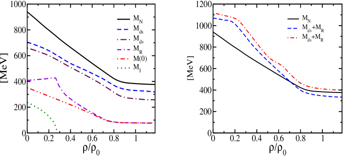
Figure 4: On the left the zero-momentum constituent quark mass $M(0)$ and the (real, imaginary) part of the first pole of the dressed quark propagator ($M_{R}$, $M_{I}$) are displayed as a function of density $\rho$ in the unit of the nuclear matter density $\rho_{0}$. We also show the effective nucleon $M_{N}$ and the diquark masses $M_{ds},M_{da}$ (for $g_{v}=0$) at finite density. On the right we show the fictitious scalar, axial diquark-quark threshold $M_{ds}+M_{R}$ and $M_{dv}+M_{R}$, respectively as a function of density $\rho/\rho_{0}$ (the nucleon mass $M_{N}$ is also shown).

In Fig. 4 (left panel) we show the effective quark mass obtained as the solution of the finite-density gap equation (30), the scalar diquark mass $M_{ds}$ and the axial-diquark mass $M_{da}$ at finite density. The density dependent nucleon mass obtained from Faddeev Eq. (19) is also shown. Notice that the nucleon mass does not follow from the addition of the diquark and constituent quark masses because of the relativistic Faddeev equation.

The effective constituent quark mass in the nuclear matter decreases with a different slope compared to that in the quark matter background non-s2 . This indicates that the many-body effect felt by a constituent quark in the nucleon is different from the quark matter. In Fig. 4 (left panel) we also show the real $M_{R}(\rho)$ and imaginary $M_{I}(\rho)$ part of the first pole of the dressed quark propagator as a function of nuclear matter density. The deconfinement occurs where $M_{I}(\rho)=0$, this corresponds to $\rho/\rho_{0}=0.28$. The real part of the first pole of the dressed quark propagator $M_{R}$ increases with density up to the deconfinement point and then it decreases and approaches the zero-momentum constituent quark mass $M(0)$ near the nuclear matter density $\rho_{0}$. In our model, we do not have a well-defined quark-diquark threshold. However, one may define a fictitious quark-diquark threshold as $M_{ds}+M_{R}$ (or $M_{da}+M_{R}$), where $M_{R}$ is the real part of the first pole of the dressed quark propagator. It is noted from Fig .4 (right panel) that the nucleon mass remains below the fictitious scalar diquark-quark threshold for all densities. However, it moves slightly above the fictitious axial diquark-quark threshold near the nuclear matter density $\rho_{0}$. Note that we show in Fig. 4 only the real part of nucleon mass. Above the diquark-quark threshold nucleon pole position is moved in the complex plane where the real part is taken as physical mass. Our numerical procedure (see Appendix) is valid when nucleon solution is not far above the fictitious threshold. It is natural to assume that at some point as we increase the density, nucleons decay to quarks and diquarks due to deconfinement. At the moment, we do not know yet the order of a possible deconfinement transition and its critical density. Based on our model approach, one can not address such questions quantitatively.

The scalar and the axial-diquark masses in medium decrease in a very similar way. Therefore, their relative importance in the nucleon description remains almost the same at different densities. The nucleon mass compared with the diquarks and the quarks has a bigger decreasing slope at very low density. However, it tends to saturate near the nuclear matter density. This effect is also observed for the diquarks, however, less pronounced.

The stabilisation of the nucleon mass $M_{N}$ at about nuclear matter density and the dynamical partial restoration of the chiral symmetry may closely be interconnected. This can be realized, since after chiral restoration of the constituent quark mass, the nucleon cannot feel the presence of the nuclear medium any more. The medium is incorporated via the quark propagator Eq. (8) through the finite-density gap equation (30) into the diquark and consequently in the diquark-quark Bethe-Salpeter equations. The Pauli-blocking effect in the medium is not present for the quarks since in the medium we do not have a quark matter background. We employ the quarks only to construct the nucleons and assume that they are not resolved by the medium. The stabilisation of the nucleon mass in nuclear matter is the same as before. In the local NJL model where quark confinement is simulated by introducing an infrared cutoff the stability of the nucleon mass is reached at higher density under2 . In the context of the derivative scalar coupling model this phenomenon is related to dynamical screening of the effective coupling dsg . In our model, it is derived from the non-locality of the underlying theory.

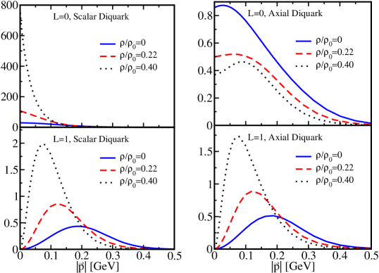
Figure 5: We show the density function of the scalar and axial diquark components within the nucleon at a given nuclear matter density $\rho$ with respect to relative momentum between diquark and quark. All given components have spin $S=1/2$ but different orbital angular momenta $L$ as indicated in the plot.

In order to find a better understanding of the internal structure of the nucleon in medium, we construct the spectator quark momentum distribution function within nucleon me1 as a function of nuclear matter density in terms of various diquark components in the nucleon rest frame,

$$\rho(|\vec{p}|,M_{N}) = \int dp_{4}\psi^{{\dagger}5}(|\vec{p}|,p_{4},M_{N})(D^{5}(p_{d}))^{-1}\psi^{5}(|\vec{p}|,p_{4},M_{N})$$ (32)

$$+ \int dp_{4}\psi^{{\dagger}\mu\nu}(|\vec{p}|,p_{4},M_{N})(D^{\mu\alpha}(p_{d}))^{-1}\psi^{\alpha\nu}(|\vec{p}|,p_{4},M_{N}),\$$

where $\psi^{{\dagger}5}$ and $\psi^{\mu\nu}$ are the Faddeev vertex functions obtained from Eq. (19) and $\vec{p}$ stands for the space component of relative momentum $p$. $D^{5}(p_{d})$ and $D^{\mu\nu}(p_{d})$ denote the diquark propagators. Although this definition is not unique, it provides some useful information about the nature of compositeness of the nucleon and their response to the medium. Note that the nucleon vertex function contains information about the compositeness of the diquark through the diquark vertex function $\chi^{5,\mu}$, see Eqs. (18,25).

In the rest frame the mass of the nucleon and its total angular momentum are good quantum numbers. In the rest frame it is also possible to decompose the nucleon vertex function in terms of tri-spinor in different diquark channels each possessing definite orbital angular momentum and spin which allows a direct interpretation of different components o1 ; me1 . The results are shown in Fig. 5. It is observed that at finite density the s-wave in the scalar diquark channel is the dominant contribution to the nucleon ground state. As the nuclear matter density increases the scalar and the axial diquark masses decrease, consequently the diquark interaction couplings $g_{s}$ and $g_{a}$ grow. This effect can be realized from Fig. 5, since the maximum strength of the density function increases as we increase the baryonic density. It is interesting to notice that from Fig. 5 one can observe that the relative importance of the scalar and axial diquarks remains intact in medium (at least at low density). In order to estimate the change of the nucleon size in response to nuclear matter environment, we compute $p_{\text{RMS}}=(\langle\vec{p}^{2}\rangle-\langle\vec{p}\rangle^{2})^{1/2}$ at finite density. This leads to $p_{\text{RMS}}\text{(MeV)}=232,182,146$ for $\rho/\rho_{0}=0,0.22$ and $0.40$, respectively. Therefore, as baryonic density increases the nucleon size grows. An increase about $35\%$ is found for density $\rho/\rho_{0}\approx 0.40$.

Fig. 6 shows the binding energy per nucleon as a function of density. The equation of state when the internal structure of nucleon are taken into account in a presence of a vector field indeed saturates. We adjust the vector mean field coupling $g_{v}$ in order to have right binding energy per particle $E_{B}/A=-16$ MeV. This corresponds to $\rho/\rho_{0}=0.60$ when $g_{v}=g_{\pi}/2.4$. The fact that the equation of state curve cannot pass exactly through the empirical saturation point implies that our hybrid approach based on a mean field approximation in the medium is still a very crude approximation.

It is well known that in the chiral models the stability of the nuclear matter depends very much on the dynamical chiral restoration sa-1 ; sa-2 ; under2 ; lastamir . The necessary condition for saturation of nuclear matter in any relativistic mean field theory is that nucleon attraction mediated from the $\sigma$-meson exchange should decrease at high density. Therefore, if $\sigma$-meson mass decreases too rapidly with density due to chiral restoration, it may work against the stabilization of the system sa-1 ; sa-2 ; under2 ; lastamir . However, as we have numerically proven, it is in principle possible to obtain a saturating nuclear matter equation of state, if the scalar field couples with the quarks instead of directly with the nucleons (see also under2 ). To this end, the nucleon is taken as a diquark-quark state which moves in self consistent scalar and vector fields coupling to the quarks.

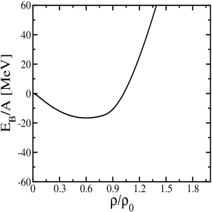
Figure 6: Energy per baryon as a function of $\rho/\rho_{0}$ ($\rho_{0}$ is nuclear matter density), for parameter set C, when $g_{v}=g_{\pi}/2.4$.

V Conclusion

In this paper we have investigated the nuclear matter in a non-local NJL model. We have worked out the equation of state of the nuclear matter in a hybrid approximation. First, we constructed the nucleon as a bound state of a diquark and a quark in the relativistic Faddeev approach and then built up nuclear matter by means of these composite nucleons. In this way, we incorporated the internal quark structure of the nucleon in a very simple framework. We showed that in this approximation the binding energy saturates. This is in contrast to the local NJL model, where in a similar framework, a stable normal nuclear matter does not exist unless one introduces a new extra parameter into the model either by including an $8$-Fermi interaction term sa-1 to induce the original coupling of the model density dependent or an infrared cutoff to simulate the confinement effect under2 ; under2-3 . Therefore, the long standing problem of matter stability in the NJL model can be resolved by introducing non-locality without invoking any adhoc new parameters. Note that the form factor Eq. (13) does not introduce any new parameter except the cutoff $\Lambda$ which is also present in the local NJL model.

We have also studied the nucleon properties such as the modification of the nucleon mass and size in a nuclear matter medium. The nucleon mass in the medium decreases very rapidly but saturates near the nuclear matter density $\rho_{0}$. We obtained the nucleon wave function from the Faddeev equation and showed that the nucleon size significantly increases in the medium. This implies a swollen nucleon in nuclear matter which has many attendant consequences bag2 ; bag1 ; last1 ; last2 . Our estimation of in-medium nucleon size should be taken more qualitatively since the quark density function given in Eq. (32) has not a unique definition. We found that the swelling of the nucleon is about $35\%$ at about half nucleon matter density. One should note that in our model at nuclear matter saturation density $\rho=0.6\rho_{0}$ the “confinement” mechanism is no longer at work, see Fig. 4 (left panel) and the nucleon becomes close to the fictitious diquark-quark threshold, see Fig. 4 (right panel). Moreover, since the nucleon mass saturates at high density, the nucleon will not expand forever. Other studies have predicted different values. For an example, it has been shown within the Friedberg-Lee nontopological-soliton bag model that the swelling of the nucleon is about $30\%$ at normal nuclear matter density bag2 . In the Skyrmion picture nucleon swelling about $40\%$ has been reported last1 . It has been also shown that in the quark-meson coupling model nucleon swelling about $25-35\%$ in saturated nuclear matter can explain the observed depletion of the structure function in the medium Bjorken $x$ region last2 .

We have also investigated the role of diquarks within the nucleon in the nuclear matter medium. The scalar and axial diquark masses decrease with a very similar slope in the medium. Despite the fact that the nucleon mass decreases (and its size increases) significantly, the role of the scalar and the axial diquark in the nucleon description remains almost the same in the nuclear medium.

In this paper, for simplicity we assumed that the auxially vector field to be local. The role of the vector meson in medium is still an open question and it deserves further investigation in our model as well.

Appendix A Numerical method

There are some subtleties involved in evaluating loop integrals as of Eq. (11) in Euclidean space. For simplicity this integral is evaluated at the timelike momentum $q=(0,iq_{0})$ in Euclidean space. For the confining parameter set, each quark propagator has a pair of complex conjugate poles. As we increase $q_{0}$, these poles in $S(p_{\pm})$ (where $p_{\pm}=p\pm\frac{1}{2}q$) have a chance to cross the real axis and may produce an imaginary part in the meson (or diquark) propagator when a threshold for decay of a meson (or diquark) into $qq$- unphysical states opens, see Fig. 9. Therefore, the standard Wick rotation of the integration contour cannot be applied. We use the prescription proposed by Cutkosky et al. cutk and successfully applied to such models in Refs. pb ; a1 ; u . This amounts to a deformation of the integration contour (as indicated in Fig. 10) to ensure that the meson or diquark propagator does not develop an imaginary part, when the first pair of complex poles of quark propagator cross the real axis. At the pinch point, both the naive integral over Euclidean four-momentum and the residue contribution diverge, although these divergences cancel to leave a finite result pb ; cutk .

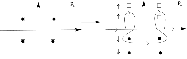
Figure 7: We show the first complex conjugate poles of loop integrals in the $p_{4}$ plane. On the left panel, the pole positions at $q_{0}=0$ are shown. The open boxes and filled circles denote the poles of the $p_{-}$ and $p_{+}$, respectively. On the right panel, we show the deformed integration contour beyond the pinch point.

The diquark-quark loops in the Faddeev equation (19) are computed in the rest frame of the nucleon $P=(E,0)$. First, we identify the singularities involved in the kernel of Faddeev equation (25) with respect to the integration momentum $k_{0}$. The singularities from quark propagator will occur at :

$$\text{pole 1}:\hskip 28.45274ptk_{0}=-\eta E+\omega^{q}_{k}-i\epsilon,$$ (33)

$$\text{pole 2}:\hskip 28.45274ptk_{0}=-\eta E-\omega^{q}_{k}+i\epsilon,\$$ (34)

where $\omega^{q}_{k}=\sqrt{k^{2}+M_{R}^{2}}$. The singularities from diquark propagator occurs:

$$\text{pole 3}:\hskip 28.45274ptk_{0}=(1-\eta)E+\omega^{d}_{k}-i\epsilon,$$ (35)

$$\text{pole 4}:\hskip 28.45274ptk_{0}=(1-\eta)E-\omega^{d}_{k}+i\epsilon,\$$ (36)

where we define $\omega^{d}_{k}=\sqrt{k^{2}+M_{d}^{2}}$ and $M_{d}$ is the the lower-energy pole in the diquark $T$-matrix (the mass of the lighter diquark). The exchanged quark propagator is also singular at:

$$\text{pole 5}:\hskip 28.45274ptk_{0}=-p_{0}+\omega^{q}_{p+k}+(1-2\eta)E-i\epsilon,$$ (37)

$$\text{pole 6}:\hskip 28.45274ptk_{0}=-p_{0}-\omega^{q}_{p+k}+(1-2\eta)E+i\epsilon,\$$ (38)

with $\omega^{q}_{p+k}=\sqrt{(k+p)^{2}+M_{R}^{2}}$. Note that all masses in the above equations are density dependent. We define

$$\alpha(\rho)=(1-\eta)M_{R}(\rho)-\eta M_{d}(\rho)\hskip 28.45274pt\eta\in[0,1].$$ (39)

It is easy to verify that in the complex $k_{0}$, the poles $2$ and $4$ lie always left of $k_{0}=\alpha(\rho)$ and poles $1$ and $3$ lie always right of $k_{0}=\alpha$ for $E<M_{R}+M_{d}$. To avoid the singularities of the kernel, we perform a Wick rotation at a given density on the energy variables around $k_{0}=\alpha(\rho)$, i. e. $k_{0}\to\alpha(\rho)+ik_{1}$ ($-\infty<k_{1}<+\infty$). Although $\alpha$ changes with density, it is in principle independent of the Mandelstam parameter $\eta$. This provides an internal check on numerical procedure. In Refs. njln3 ; walet , the parameter $\eta$ is taken $1/2$ from the outset. The location of the quark exchanged poles $5$ and $6$ depends on the $p_{0}$. One needs to bend the integration contour in such a way that the pole $5$ and $6$ to lie right and left of the path, respectively. To this end, we continue the momentum $p_{0}$ to complex plane with $p_{0}=\alpha(\rho)+ik_{2}$ then the poles $5$ and $6$ lie always right and left of the integration path $k_{0}=\alpha(\rho)+ik_{1}$. Above the diquark-quark threshold the solution of the effective Faddeev equation should be searched in complex $P^{2}$-plane. In this case the complex pole coordinates $P^{2}=E^{2}-i\gamma$ are interpreted as a mass, $E$, and $\gamma$ is related to a corresponding width com-m . Our numerical method is valid when the location of the complex pole is close to the real axis and we concentrate only on computation of the mass. In practice, one may increase the stability of the numerical procedure by taking advantage of $\eta$ (in order to escape the above-mentioned poles far enough away). This implies that one can find a plateau within the range $0<\eta<1$ where the results do not depend on the parameter $\eta$ me1 ; o1 ; o2 . The resulting complex coupled integral equations are solved by using the algorithm introduced by Oettel et al. o1 ; o2 (see also Ref.me1 ).

References

- (1) For a review see: S. P. Klevansky, Rev. Mod. Phys. 64, 649 (1992).
- (2) V. Koch, T. S. Biro, J. Kunz and U. Mosel, Phys. Lett. B185, 1 (1987).
- (3) J. Da Providencia, M. C. Ruivo and C. A. De Sousa, Phys. Rev. D36, 1882 (1987).
- (4) M. Buballa, Nucl. Phys. A611, 393 (1996).
- (5) W. Bentz and A. W. Thomas, Nucl. Phys. A696, 138 (2001).
- (6) B. D. Serot and J. D. Walecka, Int. J. Mod. Phys. E6,515 (1997); Adv. Nucl. Phys. 16,1 (1986).
- (7) For an example: T. Schafer, E. V. Shuryak, J. J. M. Verbaarschot, Nucl. Phys. B412,143 (1994).
- (8) N. Ishii, W. Bentz, K. Yazaki, Nucl. Phys. A587,617 (1995).
- (9) O. Nachtmann and H. J. Pirner, Z. Phys. C21, 277 (1984).
- (10) J. R. Smith, G. A. Miller, Phys. Rev. C65, 055206 (2002); Phys. Rev. Lett. 91, 212301 (2003).
- (11) I.C. Cloet, W. Bentz and A. W. Thomas, Phys. Rev. Lett. 95, 052302 (2005).
- (12) D. Diakonov, V. Yu. Petrov, Sov. Phys. JETP 62, 204 (1985); Nucl. Phys. B245, 259 (1984); D. Diakonov, V. Yu. Petrov, P. V. Pobylitsa, Nucl. Phys. B306, 809 (1988); I. V. Anikin, A. E. Dorokhov and L. Tomio, Phys. Part. Nucl. 31, 509 (2000).
- (13) R. D. Bowler and M. C. Birse, Nucl. Phys. A582, 655 (1995); R. S. Plant and M. C. Birse, Nucl. Phys. A628, 607 (1998).
- (14) J. Skullerud, D. B. Leinweber and A. G. Williams, Phys. Rev. D64, 074508 (2001).
- (15) R. S. Plant and M. C. Birse, Nucl. Phys. A703, 717 (2002).
- (16) A. Scarpettini, D. G. Dumm and N. N. Scoccola, Phys. Rev. D69, 114018 (2004).
- (17) W. Broniowski, B. Golli and G. Ripka, Nucl. Phys. A703, 667 (2002); B. Golli, W. Broniowski and G. Ripka, Phys. Lett. B437, 24 (1998).
- (18) A. H. Rezaeian, N. R. Walet and M. C. Birse, Phys. Rev. C70, 065203 (2004).
- (19) D. G. Dumm and N. N. Scoccola, Phys. Rev. D65, 074021 (2002).
- (20) I. General, D. G. Dumm and N. N. Scoccola, Phys. Lett. B506, 267 (2001); D. G. Dumm and N. N. Scoccola, Phys. Rev. C72, 014909 (2005); R. S. Duhau, A. G. Grunfeld and N. N. Scoccola, Phys. Rev. D70, 074026 (2004).
- (21) A. Buck, R. Alkofer and H. Reinhardt, Phys. Lett. B286, 29 (1992); S. Huang and J. Tjon, Phys. Rev. C49, 1702 (1994); H. Asami, N. Ishii, W. Bentz and K. Yazaki, Phys. Rev. C51, 3388 (1995); C. Hanhart and S. Krewald, Phys. Lett. B344, 55 (1995).
- (22) M. Oettel, G. Hellstern, R. Alkofer and H. Reinhardt, Phys. Rev. C58, 2459, (1998).
- (23) G. Hellstern, R. Alkofer, M. Oettel and H. Reinhardt, Nucl. Phys. A627, 679 (1997); M. Oettel, R. Alkofer and L. von Smekal, Eur. Phys. J. A8, 553 (2000); S. Ahlig, R. Alkofer, C.S. Fischer, M. Oettel, H. Reinhardt and H. Weigel, Phys. Rev. D64, 014004 (2001); M. Oettel, L. Von Smekal, R. Alkofer, Comput. Phys. Commun. 144, 63 (2002).
- (24) A. H. Rezaeain, hep-ph/0507304.
- (25) C. D. Roberts and A. G. Williams, Prog. Part. Nucl. Phys. 33, 477 (1994); C. D. Roberts and S. M. Schmidt, Prog. Part. Nucl. Phys. 45, S1 (2000).
- (26) H. Ito, W. W. Buck and F. Gross, Phys. Lett. B248, 28 (1990); H. Ito, W. Buck and F. Gross, Phys. Rev. C43, 2483 (1991).
- (27) T. Schäfer and E. V. Shuryak, Rev. Mod. Phys. 70, 323 (1998); D. Diakonov, Prog. Part. Nucl. Phys. 36, 1 (1996).
- (28) G. V. Efimov and S. N. Nedelko, Phys. Rev. D51, 176 (1995); Y. V. Burdanov, G. V. Efimov, S. N. Nedelko and S. A. Solunin, Phys. Rev. D54, 4483 (1996).
- (29) D. Atkinson and D. W. E. Blatt, Nucl. Phys. B151, 342 (1979).
- (30) P. Maris and H. A. Holties, Int. J. Mod. Phys. A7, 5369 (1992); S. J. Stainsby and R. T. Cahill, Int. J. Mod. Phys. A7, 7541 (1992); P. Maris, Phys. Rev. D50, 4189 (1994).
- (31) P. Maris, Phys. Rev. D52, 6087 (1995).
- (32) H.G. Dosch and S. Narison, Phys. Lett.B417,173 (1998).
- (33) L. Giusti, F. Rapuano, M. Talevi and A. Vladikas, Nucl. Phys. B538, 249 (1999).
- (34) M. Buballa, Phys. Rept. 407,205 (2005).
- (35) M. Lutz, S. Klimt and W. Weise, Nucl. Phys. A542, 521 (1992).
- (36) J. Meyer, G. Papp, H. J. Pirner, T. Kunihiro, Phys. Rev. C61, 035202 (2000).
- (37) J. Zimanyi and S. A. Moszkowski, Phys. Rev. C42, 1416 (1990); R. Aguirre and A. L. De Paoli, Eur. Phys. J. A13, 501 (2002).
- (38) For examples: J. V. Noble, Phys. Rev. Lett. 46, 412 (1981); F. E. Close, R. G. Roberts, G. G. Ross, Phys. Lett. B129, 346 (1983); M. Jandel,G. Peters, Phys. Rev. D30, 1117 (1984); R. L. Jaffe, F. E. Close, R. G. Roberts, G. G. Ross, Phys. Lett. B134, 449 (1984); L. S. Celenza, A. Rosenthal and C. M. Shakin, Phys. Rev. C31, 232 (1985); G. Chanfray, H. J. Pirner, Phys. Rev. C35, 760 (1987).
- (39) M. Jandel, G. Peters, Phys. Rev. D30, 1117 (1984).
- (40) M. Rho, Phys. Rev. Lett. 54, 767 (1985).
- (41) X. Jin, B. K. Jennings, Phys. Rev. C54, 1427 (1996); Phys. Rev.C55, 1567 (1997).
- (42) R. E. Cutkosky, P. V. Landshoff, D. I. Olive and J. C. Polkinghorne, Nucl. Phys. B12, 281 (1969).
- (43) M. S. Bhagwat, M. A. Pichowsky and P.C. Tandy, Phys. Rev. D67, 054019 (2003).
- (44) S. Pepin, M. C. Birse, J. A. McGovern and N. R. Walet, Phys. Rev. C61, 055209 (2000).
- (45) A. H. Rezaeian, nucl-th/0512027.
- (46) I. C. Cloet, W. Bentz and A. W. Thomas, Phys. Rev. Lett. 95, 052302 (2005).
- (47) V. Bernard, A. H. Blin, B. Hiller, Y. P. Ivanov, A. A. Osipov and U. G. Meissner, Phys. Lett. B409, 483 (1997).