From Finite Nuclei to the Nuclear Liquid Drop: Leptodermous Expansion Based on the Self-consistent Mean-Field Theory

Abstract

The parameters of the nuclear liquid drop model, such as the volume, surface, symmetry, and curvature constants, as well as bulk radii, are extracted from the non-relativistic and relativistic energy density functionals used in microscopic calculations for finite nuclei. The microscopic liquid drop energy, obtained self-consistently for a large sample of finite, spherical nuclei, has been expanded in terms of powers of $A^{-1/3}$ (or inverse nuclear radius) and the isospin excess (or neutron-to-proton asymmetry). In order to perform a reliable extrapolation in the inverse radius, the calculations have been carried out for nuclei with huge numbers of nucleons, of the order of $10^{6}$. The Coulomb interaction has been ignored to be able to approach nuclei of arbitrary sizes and to avoid radial instabilities characteristic of systems with very large atomic numbers. The main contribution to the fluctuating part of the binding energy has been removed using the Green’s function method to calculate the shell correction. The limitations of applying the leptodermous expansion to actual nuclei are discussed. While the leading terms in the macroscopic energy expansion can be extracted very precisely, the higher-order, isospin-dependent terms are prone to large uncertainties due to finite-size effects.

I Introduction

Bulk properties of atomic nuclei that depend in a smooth way on the numbers of nucleons have been traditionally described in terms of macroscopic models, e.g., the liquid drop model (LDM) or the droplet model; for reviews, see Refs. [Mye77] ; [Mye82] ; [Has88] ; [Mol95] ; [Pom02] . These phenomenological models, often augmented by a shell correction which is calculated using average single-particle potentials, have been tuned up to describe nuclear bulk properties to a high precision. At the same time, these models can be interpreted in the language of the leptodermous expansion [Gra82] that sorts the various contributions to the binding energy of finite nuclei in terms that have transparent physical meaning, e.g., volume, surface, symmetry, curvature, and Coulomb energy.

On the microscopic side, self-consistent mean-field models employing density-dependent effective interactions or energy-density functionals are nowadays commonly used in nuclear structure modeling. The most prominent of these are the Skyrme-Hartree-Fock (SHF) method, the relativistic mean-field (RMF) approach (as well as their Bogoliubov extensions), and the Hartree-Fock-Bogoliubov method with the finite-range Gogny force; for a recent review, see Ref. [Ben03] . These models rely on effective energy-density functionals with typically 6-10 parameters adjusted phenomenologically that provide a global description of all nuclei throughout the nuclear chart (with exception, perhaps, of the lightest ones). While the parameters of these models can be organized and interpreted using the low-energy effective field theory of quantum chromodynamics [Fur97] ; [Fur97a] ; [Bur02] , they do not have an immediate interpretation in terms of the total number of nucleons (or nuclear radius) and neutron excess. For that reason, it is both convenient and practical [Ber05] to characterize nuclear energy-density functionals in terms of certain macroscopic parameters. The usual starting point is the limit of the homogenous infinite nuclear matter, which is simple to compute and which defines the leading LDM characteristics, e.g., the volume energy, symmetry energy, or incompressibility.

Nuclei have a pronounced surface; hence, a proper characterization of surface properties is crucial. This task, however, is far from easy. The usual means of characterizing surface properties of the energy functional is through semi-infinite nuclear matter having a planar surface zone (see Ref. [Cen98a] and references quoted therein). Early attempts used semi-classical approaches to circumvent the enormous complexity of self-consistent calculations for the corresponding mean field (see, e.g., Ref. [Bra85] for the case of SHF). The limited self-consistent calculations in SHF [Pea94] ; samyn and RMF [Eif94a] indicate that the quantum effects are non-negligible to the extent that they change the surface parameters by about 5 $\%$.

In Ref. [Dob02c] the volume and surface contributions to the energy density were extracted by assuming the Thomas-Fermi relation between the local density and the kinetic energy density. The authors concluded that, in the nuclear surface zone, the gradient terms (absent in the homogenous nuclear matter) are as important in defining the energy relations as those depending on the local density. That is, the nuclear surface cannot simply be regarded as a layer of nuclear matter at low density.

In this work, we extract the macroscopic LDM parameters by using a large sample of finite, spherical nuclei, including huge systems having $10^{5}$-$10^{6}$ nucleons. Based on the self-consistent SHF and RMF results, we extract the macroscopic information from the large-scale trends by subtracting fluctuating shell corrections. The Coulomb force is switched off to allow computation of very large nuclei. (We thus concentrate on the strong component of the nuclear interaction.) This way of analysis, using finite nuclei rather than semi-infinite matter, is conceptually closer to existing nuclei, and it allows the determination of curvature and surface symmetry effects. In essence, the aim of this paper is two-fold. First, by considering finite, although huge, nuclei, we investigate the convergence of the macroscopic expansion. Second, by taking several SHF and RMF energy functionals, we explore the relation between surface parameters and the nuclear matter features of the underlying forces.

The paper is organized as follows. Section II discusses the macroscopic energy expansions. The details of our SHF and RMF models and shell-correction calculations are given in Sec. III. The extraction of LDM parameters is described in Sec. IV; they are discussed in Sec. V. Finally, conclusions are drawn in Sec. VI.

II The macroscopic energy

According to the Strutinsky Energy Theorem [Str67] ; [Str68] ; [Bra75] ; [Bra81] , the energy per nucleon can be decomposed into an average part (smoothly depending on the number of nucleons) and the shell-correction term that fluctuates with particle number reflecting the non-uniformities (bunchiness) of the single-particle level distribution:

$$\frac{E}{A}={\cal E}={\cal E}^{\rm(smooth)}+\delta{\cal E}^{\rm(shell)}.$$ (1)

Macroscopic models, such as LDM, deal with the smooth part. Consequently, in the following we concentrate on the average part of the binding energy:

$${\cal E}^{\rm(smooth)}=\frac{E}{A}-\delta{\cal E}^{\rm(shell)}\quad.$$ (2)

The macroscopic energy can be parametrized in many ways. However, by far the most successful macroscopic mass expressions are those rooted in the liquid-drop model (LDM) and in the droplet model. They are respectively outlined in Sec. II.1 and Sec. II.2 below.

II.1 Liquid-drop model

The LDM parameterizes the binding energy of the nucleus ($Z$, $N$) in equilibrium. Instead of proton and neutron numbers, it is convenient to express the LDM energy through the mass number and neutron excess:

$$A=N+Z\quad,\quad I=\frac{N-Z}{N+Z}\quad.$$ (3)

The macroscopic binding energy per nucleon can be expanded as

$$\begin{array}[]{rclclcl}\displaystyle{\cal E}^{\rm(LDM)}&=&\lx@intercol{\cal E}^{\rm(smooth)}(A,I)\hfil\lx@intercol\\ &=&a_{\rm vol}&+&a_{\rm surf}A^{-1/3}&+&a_{\rm curv}A^{-2/3}\\[4.0pt] &&&+&a_{\rm sym}I^{2}&+&a_{\rm ssym}I^{2}A^{-1/3}\\[5.0pt] &&&&&+&a_{\rm sym}^{(2)}I^{4}\quad.\end{array}$$ (4)

All the terms in Eq. (4) have an immediate physical interpretation. The bulk energy is given by the volume energy $a_{\rm vol}$, and changes with the neutron excess are accounted for by the symmetry-energy term $a_{\rm sym}I^{2}$ and by the second-order symmetry-energy term $a_{\rm sym}^{(2)}I^{4}$. The most important finite-size correction is the surface energy $a_{\rm surf}A^{-1/3}$, followed by more subtle trends in terms of the curvature energy $a_{\rm curv}A^{-2/3}$ and the surface-symmetry energy $a_{\rm ssym}I^{2}A^{-1/3}$.

The sorting in columns indicates the level of importance of the terms. Two different sorting criteria are used simultaneously: an expansion of finite size effects (=surface effects) in terms of powers of $A^{-1/3}$ (proportional to inverse radii) and, parallel to it, an expansion in terms of the neutron-to-proton asymmetry $I^{2}$. The second-order symmetry energy term $\propto I^{4}$ is not always included in the macroscopic binding energy expression. It has been considered, e.g., in the context of the Thomas-Fermi model [Mye98b] and in a discussion of strongly asymmetric matter within the RMF [Liu02a] . We find that such a term appears naturally in the hierarchy of Eq. (4), and we shall demonstrate that it is naturally present in the microscopic LDM expression.

At this point, it is worth noting that the shell energy per nucleon, $\delta{\cal E}^{\rm(shell)}$, scales with mass as $A^{-2/3}$ [Boh75] , i.e., it has the same dependence on the nuclear radius as the curvature term. Consequently, uncertainties associated with the extraction of shell corrections from self-consistent results, and the presence of higher-order fluctuating terms that are not accounted for by the Strutinsky procedure, can seriously impact the values of higher-order terms in the leptodermous expansion. We will see it very clearly in the results presented in Sec. IV.

The ansatz (4) does not include explicit information about the nuclear radius. In fact, the LDM tacitly assumes a fixed radius

$$R_{0}=r_{s}A^{1/3}$$ (5)

where the Wigner-Seitz radius is typically $r_{s}=$1.14-1.20 fm, which defines the saturation (equilibrium) density

$$\rho_{0}=\frac{3}{4\pi r_{s}^{3}}\quad.$$ (6)

A more general ansatz which allows a determination of the radius is provided by the droplet model presented below.

II.2 Droplet model

The droplet model [Mye74] (see, e.g., Ref. [Mol95] for a recent implementation) includes the effect of the neutron skin and non-uniformities in the nuclear density. The two crucial parameters of the droplet model that describe deviations from the equilibrium are the neutron skin thickness $d$ and $\epsilon$, the relative deviation in the bulk of the density $\rho$ from its nuclear matter value $\rho_{0}$:

$$d = R_{n}-R_{p}\quad,$$ (7a)

$${\epsilon} = \frac{R-R_{0}}{R}=-\frac{\rho-\rho_{0}}{3\rho_{0}},$$ (7b)

where $R_{0}$ is the equilibrium radius of the droplet, see eq. (5). Energy changes with $d$ and $\epsilon$ are considered explicitly. For instance, the volume term is augmented by a compression effect,

$$a_{\rm vol}\longrightarrow a_{\rm vol}+\frac{1}{2}K\epsilon^{2}\quad,$$ (8)

where the nuclear incompressibility coefficient is

$$K\equiv 9\rho^{2}_{0}\frac{d^{2}}{d\rho^{2}}\frac{E}{A}\bigg{|}_{\rho=\rho_{0}}.$$ (9)

The droplet model binding energy per particle is considered a function of $A$, $I$, ${\epsilon}$, and $d$:

$$\begin{array}[]{rclclcl}{\cal E}^{\rm(drop)}&=&\lx@intercol{\cal E}^{\rm(drop)}(A,I,\epsilon,d)\hfil\lx@intercol\\ &=&a_{\rm vol}&+&a_{\rm surf}A^{-1/3}&+&\tilde{a}_{\rm curv}A^{-2/3}+2a_{\rm surf}A^{-1/3}{\epsilon}+\frac{K}{2}{\epsilon}^{2}\\ &&&+&a_{\rm sym}{I^{2}}&+&\tilde{a}_{\rm ssym}A^{-1/3}f(I,d)-3a^{\prime}_{\rm sym}{I^{2}}{\epsilon}+\tilde{a}^{(2)}_{\rm sym}{I^{4}}\end{array}$$ (10)

where $a^{\prime}_{\rm sym}$ is defined as

$$a^{\prime}_{\rm sym}=\frac{\partial a_{\rm sym}}{\partial\rho}\bigg{|}_{\rho=\rho_{0}}.$$ (11)

The function $f(I,d)$ is assumed to be quadratic in $I$ and $d$; it is determined by minimizing the energy with respect to $d$, see below.

II.3 Relation between droplet model and LDM expansions

In this section, we recall the relation between the LDM expression (4) and the more detailed droplet mass formula (10). The form (4) is valid at the energy in equilibrium (i.e., where radius and/or density have been adjusted to minimize the energy for a given nucleus) while equation (10) allows for separate tuning of ${\epsilon}$ and $d$. The equilibrium energy ${\cal E}^{\rm(red)}(A,I)$ is obtained by minimizing ${\cal E}^{\rm(drop)}(A,I,{\epsilon},d)$ with respect to ${\epsilon}$ and $d$. At the equilibrium, $d=bI$, where $b$$\approx$1.4  fm. For the radial expansion ${\epsilon}$, one obtains

$${\epsilon}=\frac{-2a_{\rm surf}A^{-1/3}+3a^{\prime}_{\rm sym}I^{2}}{K}\quad.$$ (12)

By substituting (12) in (10), one arrives at the LDM expression (4) where the leading parameters $a_{\rm vol}$, $a_{\rm surf}$, and $a_{\rm sym}$ remain unchanged while the higher-order parameters are redefined as:

$$a_{\rm curv} = \tilde{a}_{\rm curv}-2a_{\rm surf}^{2}\frac{\rho_{0}^{2}}{K}\quad,$$ (13a)

$$a_{\rm ssym} = \tilde{a}_{\rm ssym}-6a_{\rm surf}a^{\prime}_{\rm sym}\frac{\rho_{0}^{2}}{K}\quad,$$ (13b)

$$a^{(2)}_{\rm sym} = \tilde{a}^{(2)}_{\rm sym}-\frac{9}{2}(a^{\prime}_{\rm sym})^{2}\frac{\rho_{0}^{2}}{K}\quad.$$ (13c)

It is seen that while the leading parameters, $a_{\rm vol}$, $a_{\rm surf}$, and $a_{\rm sym}$, are defined unambiguously in both LDM and droplet model expressions, the higher-order terms differ. We shall determine the parameters of the leptodermous expansion from the calculated ground state binding energies. The corresponding mean-field configurations are stable points; hence, the equilibrium philosophy of the LDM should apply. To deduce the droplet model parameters $\tilde{a}_{\rm curv}$, $\tilde{a}_{\rm ssym}$, and $\tilde{a}^{(2)}_{\rm sym}$, one should use the relations (13).

Table 1: LDM coefficients (in MeV) for the self-consistent mean-field models applied in this work. The first block (columns 2 and 3) shows, for reasons of completeness, bulk droplet-model parameters $\rho_{0}$ and $K$. The second block (columns 4-6) shows the bulk parameters of the LDM as computed in the limit of homogenous nuclear matter. The third block (semi-bulk; column 7) shows surface parameters from semi-infinite nuclear matter calculations, where available (Ref. samyn for SHF and Ref.  [Eif94b] for RMF). The results for the parameters deduced from finite nuclei as described below are shown in columns 8-10. The theoretical uncertainty on surface energies is 0.05 MeV for SHF and 0.1 MeV for RMF. The curvature energies are reliable within 0.5 MeV. The surface-symmetry energies have an uncertainty of about 2 MeV for SHF and 10 MeV for RMF. The lowest rows show the LDM coefficients adjusted to data on finite nuclei. The corresponding parameters of the droplet model (10) can be deduced from the given LDM parameters through the relations (13) plus the empirically supported assumption (16a).

	bulk properties					semi-bulk	from finite nuclei
Model	$\rho_{0}$	$K$	$a_{\rm vol}$	$a_{\rm sym}$	$a^{\prime}_{\rm sym}$	$a_{\rm surf}^{\text{(NM)}}$	$a_{\rm surf}$	${a}_{\rm curv}$	${a}_{\rm ssym}$
SkM∗	0.1603	216.6	-15.752	30.04	95.25	17.70	17.6	9	-52
SkP	0.1625	201.0	-15.930	30.01	40.43	18.22	18.2	9.5	-45
BSk1	0.1572	231.4	-15.804	27.81	15.76	17.54	17.5	9.5	-36
BSk6	0.1575	229.2	-15.748	28.00	35.67		17.3	10	-33
SLy4	0.1596	230.1	-15.972	32.01	95.97		18.4	9	-54
SLy6	0.1590	230.0	-15.920	31.96	99.48	17.74	17.7	10	-51
SkI3	0.1577	258.1	-15.962	34.84	212.47		18.0	9	-75
SkI4	0.1601	247.9	-15.925	29.51	125.80		17.7	9	-34
SkO	0.1605	223.5	-15.835	31.98	163.50		17.3	9	-58
NL1	0.1518	211.3	-16.425	43.48	311.18		18.8	9	-110
NL3	0.1482	271.7	-16.242	37.40	269.16	18.5	18.6	7	-86
NL-Z	0.1509	173.0	-16.187	41.74	299.51		17.8	9	$<$ -125
NL-Z2	0.1510	172.4	-16.067	39.03	281.40	17.7	17.4	10	-90
LDM [Mol95]	0.153		-16.00	30.56			21.1		-48.6
LDM [Pom02]	0.1417		-15.848	29.28			19.4		-38.4
LSD [Pom02]	0.1324		-15.492	28.82			17.0	3.9	-38.9

III Self-consistent Models

We employ two variants of self-consistent mean-field models: SHF and RMF. They are explained in detail in Ref. [Ben03] . Both approaches provide a functional form for the energy density with a good handful of free parameters. These have been adjusted to phenomenological data by different groups and with different bias. Thus there exist various parametrizations on the market which provide a fairly good description of basic nuclear bulk properties in the valley of stability, but differ in other aspects as, e.g., excitations, fission barriers, neutron matter properties, or electromagnetic form factors.

In this work, we have chosen a small subset of Skyrme forces which perform well for the basic ground-state properties and have sufficiently different properties which allows one to explore the possible variations among parameterizations. This subset contains: SkM^∗ [Bar82] , SkP [Dob84] , SLy4 [Cha95a] , SLy6 [Cha98] , SkO [Rei99] , BSk1 [Sam02] , BSk6 [Gor03] , and SkI1, SkI3, and SkI4 from Ref. [Rei95] . SkP, SkO, and BSk1 have effective nucleon mass around one, leading to a comparatively large density of single-particle levels. All other SHF forces employed here have smaller effective masses. Interesting here is the double BSk1 with BSk6. Both forces were fitted using a similar strategy and data pool, but have different effective mass $m^{*}/m=1.05$ for BSk1 and $0.8$ for BSk6. The force SLy6 was adjusted with particular emphasis on isotopic trends and neutron matter. The functionals SkI3, SkI4, and SkO have a generalized isovector spin-orbit interaction compared to all other forces. Some forces, i.e. SkP, BSk1, and BSk6, include a $\tensor{J}^{2}$ term (where $\tensor{J}$ is the spin-orbit tensor) with a coupling constant related to the surface and effective mass terms, while all others do not. All the selected forces perform reasonably well concerning the total energy and radii for nuclei close to the valley of stability, with some different bias on particular observables. In particular, BSk1 and BSk6 are fits to all available masses, but only masses.

As seen in Table 1, the values for the volume energy coefficient $a_{\text{vol}}$, saturation density $\rho_{0}$, incompressibity $K$, and surface energy coefficient $a_{\text{surf}}$ are quite similar, with slight systematic differences between SHF and RMF that already have been noticed earlier; see [Ben03] and references given therein. Obvious large variations occur for properties which are not fixed precisely by nuclear matter and ground-state characteristics.

As in SHF, there exist many RMF parameterizations which differ in details. For the purpose of the present study, we choose the most successful (or most commonly used) ones: NL1 [Rei86] , NL-Z [Ruf88a] , NL-Z2 [Ben99a] , and NL3 [Lal97] . The parameterization NL1 is a fit of the RMF along the strategy of Ref. [Fri86] . The NL-Z parametrization is a refit of NL1 where the correction for spurious center-of-mass motion is calculated from the actual many-body wave function, while NL-Z2 is a recent variant of NL-Z with an improved isospin dependence. The force NL3 stems from a fit including exotic nuclei, neutron radii, and information on giant resonances. All the above parameterizations provide a good description of binding energies, charge radii, and surface thicknesses of stable spherical nuclei with the same overall quality as the SHF model. As seen in Table 1, however, the nuclear matter properties of the RMF forces show some systematic differences as compared to Skyrme forces. All RMF forces have comparable small effective masses around $m^{*}/m\approx 0.6$. (Note that the effective mass in RMF depends on momentum; hence the effective mass at the Fermi energy is approximately $10\%$ larger.) Compared with SHF models, the absolute value of the energy per nucleon is systematically larger, with values around $-16.3$ MeV, while the saturation density is always slightly smaller with typical values around 0.15 nucleons/fm³. The incompressibility of the RMF forces ranges from low values around 170 MeV for NL-Z to $K$=270 MeV for NL3. There are also differences in isovector properties; the symmetry energy coefficient of all RMF forces is systematically larger than for SHF interactions, with values between 37.4 MeV for NL3 and 43.5 MeV for NL1.

The absolute variation of the LDM energy coefficients found in Table 1 should be put into perspective. There is a notable difference between the variation of the coefficients in the LDM expansion on the one hand and the actual variation of the energy on the other hand. Let us consider the heavy nucleus ²⁵⁰Fm with $A=250$ and $I=0.2$ as an example. The difference in $a_{\text{vol}}$ between SkM* and NL1 is 0.67 MeV, which seems to be small. It leads, however, to an energy difference of about 160 MeV, which amounts to a significant fraction ($\sim$10 $\%$) of the total binding energy of this nucleus. The difference in the symmetry energy coefficient, $a_{\text{sym}}$ between the same two forces is 3.44 MeV and appears to be much more significant that the difference in $a_{\text{vol}}$. However, the $I^{2}$ factor suppresses the difference in the symmetry energy between SkM* and NL1 to 34.4 MeV. Even the 60 MeV difference between the surface symmetry energy coefficients of SkM* and NL1 only gives about 100 MeV difference in binding energy between the two forces, which is comparable with, but still smaller than, the energy difference arising from the small difference in the volume energy coefficient.

It is interesting to check to what extent the differences in $\rho_{0}$, $K$, and $a^{\prime}_{\text{sym}}$ influence the macroscopic parameters and whether a simple correlation between spectroscopy and macroscopy can be found. This will be done in Sec. V.2, where we will consider a larger variety of parameterizations and perform dedicated variations of special features as, e.g., the effective nucleon mass.

According to Eq. (2), the average energy is obtained by subtracting the shell-correction energy from the self-consistent value. The shell energy is computed using the same prescription as outlined in Refs. [Kru00b] ; [Ver00] . This procedure is based on the Green’s function approach to the level density and the generalized plateau condition of Ref. [Ver98] . The advantage of this procedure is that it properly takes care of the continuum positive-energy states which unavoidably come into play in the self-consistent approach. In our calculations, we include a large space of single-particle states up to 60 MeV above the Fermi energy. Since most of these states are continuum states, the contribution from a particle gas (treated in the same numerical box) has to be removed. To meet the generalized plateau condition, it is assumed that the deviation of the smoothed level density from linearity is minimal in a wide energy interval [–50,–20] MeV.

Our calculations are restricted to spherical symmetry; they were carried out using numerical techniques described in detail in Ref. [Rei89a] . The Coulomb force is ignored to allow an extension to nuclei of arbitrary sizes. Pairing correlations are neglected as well. However, open-shell nuclei were treated in the filling approximation in which we use a very small pairing force (factor of 10 smaller than usual). The center-of-mass (c.m.) correction is included. We take care to use precisely the c.m.  recipe that is attached to a given force [Ben03] . This is crucial because it is known that the actual form of the c.m. correction has a significant impact on the surface properties [Ben00d] .

IV Extraction of LDM parameters

IV.1 Bulk parameters

The bulk parameters in the leptodermous expansion are those proportional to $A^{0}$. They represent terms which do not vanish in the $A\to\infty$ limit. In the LDM ansatz (4) the bulk parameters are: the volume energy constant $a_{\rm vol}$, the symmetry energy constant $a_{\rm sym}$, and the second-order symmetry energy parameter ${a}_{\rm sym}^{(2)}$. The droplet model (10) additionally introduces the incompressibility $K$, the density-slope of the symmetry energy $a^{\prime}_{\rm sym}$, and the equilibrium density $\rho_{0}$. All these parameters can easily be computed in the limit of the homogenous bulk nuclear matter, see, e.g., Ref. [Ben03] .

Asymmetric nuclear matter shows an interesting trend, which sheds some light on the relation between the LDM and droplet model. The bulk part of the LDM energy can be written as:

$${\cal E}^{\rm(LDM)}=a_{\rm vol}+a_{\rm sym}I^{2}+a_{\rm sym}^{(2)}I^{4}.$$ (14)

In order to concentrate on the isospin dependence, we introduce an effective symmetry energy parameter as

$$a_{\rm sym}^{\rm eff} = \frac{{\cal E}(I)-{\cal E}(I\!=\!0)}{I^{2}}$$

$$= a_{\rm sym}+a_{\rm sym}^{(2)}I^{2}\quad.$$

The first line serves as a general definition. The second line then is specific to the bulk limit.

Figure 1: Solid line: the effective symmetry energy parameter (IV.1) in asymmetric nuclear matter computed with NL-Z2 as a function of neutron excess $I$. Dotted line: the trend (16b) using the bulk parameters of NL-Z2, see Table 1.

Figure 1 shows the effective symmetry energy parameter obtained in the NL-Z2 model. Let us now recall that $a_{\rm sym}^{(2)}$ is related to the droplet parameter $\tilde{a}_{\rm sym}^{(2)}$ through Eq. (13c). This suggests that there is no explicit second-order isospin correction to the symmetry energy in the droplet model:

$$\tilde{a}_{\rm sym}^{(2)}=0,$$ (16a)

which yields

$$a_{\rm sym}^{\rm eff}(A\!=\!\infty,I)=a_{\rm sym}-\frac{9}{2}(a^{\prime}_{\rm sym})^{2}\frac{\rho_{0}^{2}}{K}I^{2}\quad.$$ (16b)

It is seen in Fig. 1 that the estimate (16b) matches the exact result extremely well. The deviations are small and predominantly $\propto I^{4}$, thus going beyond the present expansion. (Higher-order isospin corrections were in fact considered in Ref. [Liu02a] in the context of RMF and infinite nuclear matter.) We have checked that the assumption (16) is well fulfilled for all the RMF and SHF functionals used in this work. The isospin dependence of $a_{\rm sym}^{\rm eff}(A\!=\!\infty,I)$ in SHF is much weaker than in RMF. This is consistent with Eq. (16b) and droplet-model parameters displayed in Table 1. Finally, corroborating evidence of a very small $\tilde{a}_{\rm sym}$ term comes from Brueckner-Hartree-Fock studies of asymmetric matter based on realistic nucleon-nucleon and three-body forces [Bor98] ; [Zuo99] ; [Zuo02] .

IV.2 Isospin-independent surface parameters

The leading isospin-independent parameters characterizing finite-size (surface) terms in the LDM are the surface and curvature energy coefficients. We deduce them from the systematics of binding energies of spherical nuclei.

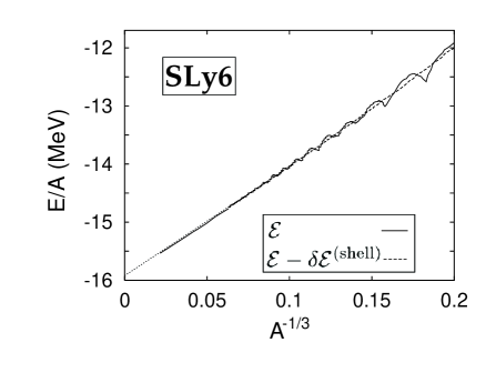
Figure 2: The binding energy per nucleon ${\cal E}(A,I)$ for isospin-symmetric ($I=0$) nuclei computed with SLy6 as a function $A^{-1/3}$ before (solid line) and after (dotted line) subtracting the shell correction $\delta{\cal E}^{\rm(shell)}$. The fine dotted line connects the last value from finite nuclei with the nuclear matter limit.

Figure 2 shows the systematics of binding energies per nucleon predicted by SLy6. The smooth component obtained by subtracting $\delta{\cal E}^{\rm(shell)}$ is also indicated. At very large values of $A$ (i.e. small $A^{-1/3}$), the binding energy per nucleon nicely converges to a straight line which demonstrates the validity of the hierarchical LDM (or droplet) ansatz and, not surprisingly, hints at the dominating role played by the surface energy as first leading correction to the bulk. The plot also illustrates the effect of quantum shell fluctuations. The actual binding energy oscillates around the average trend; the amplitude of shell oscillations increases in lighter nuclei, consistent with the expected $A^{-2/3}$-dependence discussed earlier in Sec. II.1. By subtracting the shell correction, one obtains a fairly smooth trend, at least at this level of analysis.

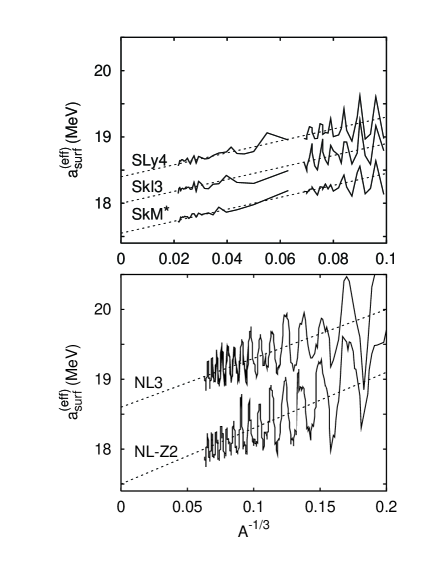
Figure 3: Effective surface-energy coefficient (17a) versus $A^{-1/3}$ for several SHF (top) and RMF (bottom) functionals, as indicated. A straight-line fit to the data is marked by a dashed line.

To extract the surface- and curvature-energy coefficients, it is convenient to introduce the effective surface-energy coefficient:

$$a_{\rm surf}^{\rm(eff)} = \big{[}{\cal E}^{\rm(smooth)}(A,0)-a_{\rm vol}\big{]}A^{1/3}$$ (17a)

$$= a_{\rm surf}+{a}_{\rm curv}A^{-1/3}\quad,$$ (17b)

which is a function of system size $A$. The surface-energy coefficient $a_{\rm surf}$ is obtained by extrapolating $A^{-1/3}\longrightarrow 0$. The curvature ${a}_{\rm curv}$ is then obtained from the slope of (17b).

Figure 3 shows the effective surface energies. Note that these are drawn from smoothed energies (i.e. after subtraction of the shell corrections). The remaining fluctuations are due to higher-order shell effects [Bra75] ; [Bra81] which cannot be accounted for by the generalized Strutinsky procedure. The construction (17a) of the effective surface energy amplifies those residual fluctuations dramatically; it is only by virtue of the smoothed energy that one can see any clear trend. Thus atop these remaining shell fluctuations, one can recognize a definite slope (note the very narrow energy window), which is related to the curvature energy. By performing a straight-line fit to the data, surface- and curvature-energy coefficients can be extracted.

Note that different $A^{-1/3}$ scales are used for SHF and RMF. The reason is that in SHF cases we have been able to carry up calculations for really huge nuclei ($A=10^{6}$). This extends the scale to smaller $A^{-1/3}$ and allows us to ignore some data points for lighter systems where residual shell fluctuations are large. Unfortunately, we were unable to approach similarly large nuclei in RMF; hence, we had to scale up to $A^{-1/3}=0.2$ to get sufficient data for extrapolation. In any case, one sees that one can extract reliably well surface and curvature energies from the trends displayed in Fig. 3. We estimate an uncertainty in $a_{\rm surf}$ to be about 0.05 MeV for SHF and 0.1 MeV for RMF. The curvature coefficient is determined within about $\pm 0.5$ MeV.

IV.3 Surface-symmetry coefficient

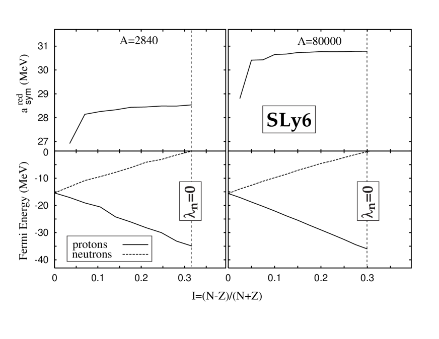
Figure 4: Top: reduced effective symmetry-energy coefficient (18) in SLy6 versus $I$ for two system sizes ($A$=2840, left; $A$=80,000, right). Bottom: corresponding proton and neutron Fermi energies.

In order to deduce the isospin-dependent surface-symmetry coefficient, we come back to the effective symmetry parameter (IV.1) now considering finite $A$ and identifying ${\cal E}\leftrightarrow{\cal E}^{\rm(smooth)}$. As it is convenient to subtract the known infinite-matter trend of Eq. (16b), we introduce the reduced effective symmetry-energy coefficient:

$$a_{\rm sym}^{\rm red}(A,I) = \frac{1}{I^{2}}\left({\cal E}^{\rm(smooth)}(A,I)-{\cal E}^{\rm(smooth)}(A,0)+\frac{9(a^{\prime}_{\rm sym})^{2}\rho_{0}^{2}}{2K}I^{4}\right)\quad.$$ (18)

Figure 4 demonstrates how such methodology works. The symmetry energy involves a difference of smoothed energies; hence, a difference of shell corrections. These corrections are prone to uncertainties, as we have already seen in Sec. IV.2. At small values of $I^{2}$, the remaining uncontrolled energy fluctuations are amplified in the finite difference (18), and the result is not reliable. Fortunately, at larger values of $I\geq 0.1$, where the isospin-dependent terms dominate over remaining shell fluctuations, one always obtains a stable and well-defined plateau. The value of $I$ is limited from above by the neutron drip line. Indeed, at $I\approx 0.3$ the neutron Fermi energy becomes positive and the self-consistent solution can no longer be trusted. Therefore, for further analysis, we introduce an $I$-averaged reduced effective symmetry-energy coefficient:

$$\overline{a_{\rm sym}^{\rm red}}={\int_{0.1}^{0.2}dI\,a_{\rm sym}^{\rm red}(A,I)}\;\left/\;{\int_{0.1}^{0.2}dI}\right.\quad.$$ (19)

The surface symmetry energy coefficient is obtained by plotting $\overline{a_{\rm sym}^{\rm red}}$ versus $A^{-1/3}$. The slope for small $A^{-1/3}$ corresponds to ${a}_{\rm ssym}$, similarly as it was done in Sec. IV.2 for deducing the surface and curvature parameters. An effective surface-symmetry constant can thus be obtained from

$${a}_{\rm ssym}^{\rm(eff)}=\left(\overline{a_{\rm sym}^{\rm red}}-a_{\rm sym}\right)A^{1/3}\quad.$$ (20)

Figure 5: Bottom: the averaged reduced symmetry-energy coefficient (19) in SLy6 and NL-Z2; Top: the corresponding effective surface-symmetry coefficient (20).

Figure 5 shows typical results of such analysis. It is gratifying to see that the effective symmetry-energy coefficients (19) are consistent with the corresponding bulk values when extrapolating back to $A^{-1/3}\to 0$. The quality of the deduced slope (= surface asymmetry) can be assessed by inspecting the rescaled quantity (20) shown in the upper panel. Clearly, very large $A$, i.e., very small $A^{-1/3}$, are required to see convergence to a strictly horizontal trend. With the present data set, one may attach $\sim$10 $\%$ relative uncertainty (or about 2 MeV absolute error) to ${a}_{\rm ssym}$.

IV.4 Radii

By employing the equilibrium value of $\epsilon$ (12), we can estimate the droplet-model radius as

$$R=R_{0}(1-{\epsilon}).$$ (21)

It is worth checking the performance of that recipe. To this end, we have extracted diffraction radii and r.m.s. radii from the SLy6 calculations of large (and huge) spherical nuclei with $N$=$Z$. Figure 6 displays the nuclear radii corrected for shell fluctuations up to $A$=4000. It is seen that the estimate (21) evaluated with the SLy6 parameters of Table 1 nicely approximates the actual results. The r.m.s. radii are systematically larger than the diffraction radii which is no surprise because in the Helm model both are related via

$$r_{\rm rms}=\sqrt{\frac{3}{5}}\sqrt{R_{\rm diff}^{2}+5\sigma^{2}}$$ (22)

where $\sigma$ is the surface thickness coefficient (related to the first maximum of the form factor) with a typical value of 1 fm. The estimate (22) is indicated in Fig. 6, and it is shown to be fully consistent with the self-consistent results for the r.m.s. radii. Moreover, our analysis makes it very clear that the diffraction radius (or box-equivalent) is indeed the appropriate quantity entering the droplet model.

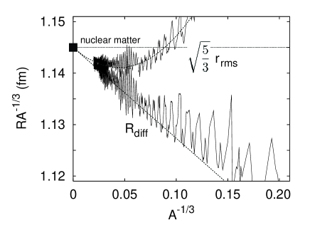
Figure 6: Nuclear radii (multiplied by $A^{-1/3}$ to remove the overall mass dependence) for $N=Z$ nuclei computed with SLy6 and (partly) corrected for shell fluctuations using the Strutinsky method. The lower curve shows the diffraction radii and the upper curve shows the r.m.s. radii $\sqrt{5/3}r_{\rm rms}$. The nuclear matter Wigner-Seitz value of 1.145 fm is indicated by a box and a horizontal dashed line. The droplet model estimate (21) of the diffraction radius and the estimate (22) of the r.m.s. radius are shown (dotted lines). It is gratifying to see the agreement between the droplet-model estimates and the results of self-consistent calculations for finite nuclei.

V Results and discussion

V.1 Existing energy functionals

Table 1 collects the calculated LDM parameters for the SHF and RMF parametrizations introduced in Sec. III. The bulk parameters are computed for the homogenous nuclear matter. The surface-related parameters are deduced from the present analysis of finite nuclei. We also show for comparison the surface-energy coefficients, $a_{\rm surf}^{\rm(NM)}$, obtained from quantum mechanical calculations for the semi-infinite nuclear matter samyn ; [Eif94b] . The comparison of $a_{\rm surf}^{\rm(NM)}$ with the values of $a_{\rm surf}$ deduced from finite nuclei shows a nice agreement between both methods of analysis.

The surface-energy and curvature-energy coefficients are fairly robust quantities in that the variations throughout all forces are small. The curvature energy coefficient, $9.5\pm 0.5$ MeV, is smaller than other LDM constants but certainly nonzero. Moreover, its variations remain small throughout all forces “from the shelves”, below the uncertainties of our analysis. In that context, we want to comment on the investigations of Ref. [Sto88b] (see also discussion in [Pom02] ) where it was claimed that one needs small curvature-energy coefficients to obtain a good fit to fission barriers. While we find about the same curvature energy for a variety of forces, the fission barriers of actinides and superheavy elements investigated in [Bur04] turned out to be strongly force-dependent for a similar pool of interactions. We suspect that another key parameter affecting fission barriers lies in the isovector channel. As one hint we will see in Sec. V.2 that strong variations of the symmetry-energy coefficient can influence $a_{\rm curv}$.

The surface energy is more important and its (small) variations are larger than the uncertainty of about $\pm 0.1$ MeV. The observed trends can be sorted in various ways. One important aspect is that $a_{\rm surf}$ depends to some extent on the strategy used when fitting a functional. It is obvious that the weight which was given to light nuclei in the fit has an influence on the surface coefficients, as well as whether surface properties were considered (e.g., the surface thickness in the case of SkI3 and SkI4). Another crucial ingredient in the trends with $A^{-1/3}$ is the way in which the center-of-mass (c.m.) correction was implemented [Ben00d] . In the sample of forces considered here, there are two forces, SLy4 and SLy6, which were fitted with precisely the same strategy but differ in their treatment of c.m. correction. The difference of 0.7 MeV in $a_{\rm surf}$ is quite remarkable and represents mainly the difference between the recipes for the c.m. correction used [Ben00d] . We think that the recipe used in SLy6, namely to compute the c.m. energy from the given mean field state, is better microscopically motivated. Thus the lower value for $a_{\rm surf}$ is probably more realistic. However, this has yet to be explored in more detail.

The situation for all the isospin-dependent LDM parameters is quite different. That begins with the large discrepancy between $a_{\rm sym}$-values for RMF and SHF. In fact, even within SHF alone there is a much larger variation in the symmetry energy than appears from Table 1; see, e.g., the discussion in Ref. [Rei99b] . Extended RMF functionals also show significant uncertainty in $a_{\rm sym}$ [Typ01] . Even more pronounced are fluctuations in the surface-symmetry coefficient $a_{\rm ssym}$. By inspecting Table 1, one can see a rough correlation between $a_{\rm sym}$ and $a_{\rm ssym}$. This will be put on a firmer ground in Sec. V.2 below where systematic variations of functionals are discussed.

V.2 Systematic variations of functionals

The discussion of Table 1 in Sec. V.1 has indicated several features which deserve closer inspection. To this end, we perform systematic variations of key properties of the functional, as, e.g. effective nucleon mass $m^{*}/m$ or symmetry energy $a_{\rm sym}$. The strategy is to vary only one chosen property while keeping all other features fixed. A set of SHF forces has been produced that way by fitting the parameters always to the same set of data (energies, charge form factors, spin-orbit splitting) while putting a constraint on the required additional feature. This was done formerly for the purpose of studying trends in the giant resonances [Rei99b] . We consider these families of functionals in this work to inspect trends and correlations in a systematic manner.

Figure 7: Dependence of LDM parameters on effective mass (left) and the symmetry-energy coefficient (right). The incompressibility is not shown in the right panel because it does not change. The curvature energy coefficient is not shown in the left panel because it varies very little as a function of $m^{*}/m$. The extended Skyrme functionals of Ref. [Rei99b] are used.

Figure 7 shows results of two sets of calculations. The first group in the left panel contains functionals with systematically varied effective mass $m^{*}/m$. The functionals belonging to the second set, shown in the right panel, vary $a_{\rm sym}$. Looking at the left panel, we find sizable variations with effective mass concerning $a_{\rm surf}$, $K$, and $a^{\prime}_{\rm sym}$. All those parameters decrease with $m^{*}/m$. The surface-symmetry coefficient $a_{\rm ssym}$ is fairly insensitive to $m^{*}/m$. The curvature energy coefficient ${a}_{\rm curv}$ (not shown here) varies only between 9 and 10 MeV which is very little in view of the theoretical uncertainty in this parameter. Different trends are seen when the variation in $a_{\rm sym}$ is considered (Fig. 7, right). There is a dramatic change of the isospin-dependent terms, namely the density-dependent symmetry-energy coefficient $a^{\prime}_{\rm sym}$ and the surface-symmetry coefficient $a_{\rm ssym}$. The magnitude of variations in $a_{\rm surf}$ is comparable to that from the first set. That is, a lower value of $a_{\rm sym}$ can compensate for a larger effective mass. (A similar conclusion, in a slightly different context, has been drawn in Ref. [Agr04] .) And here is the first time that we see a handle on the curvature coefficient $a_{\rm curv}$: it weakly decreases with $a_{\rm sym}$.

The above trends explain most of the results for the standard Skyrme functionals displayed in Table 1. However, the comparison between BSk1 and BSk6 leaves some puzzles. The functional BSk6 has a lower effective mass than BSk1 (0.8 versus 1.05), and yet, the surface-energy coefficient slightly shrinks. This can probably be related to an improved treatment of the center-of-mass correction in BSk6.

As already mentioned, there exist different prescriptions for defining the spin-orbit interaction in SHF [Ben03] . One variation concerns the possible contribution from the kinetic forces resulting in a $\tensor{J}^{2}$-term in the energy functional ($\tensor{J}$ is the spin-orbit tensor). We have studied this point within our systematic calculations. The results in Fig. 7 employ a version without (left panel) and with (right) that term. The same conditions are met for the left set at $m^{*}/m=0.81$ and the right set at $a_{\text{sym}}=32$ MeV. All quantities shown are insensitive to that change, except for the density-dependent symmetry energy coefficient $a^{\prime}_{\rm sym}$, which exhibits a surprisingly large sensitivity to $\tensor{J}^{2}$. We have checked this point in more detail and concluded that the spin-orbit tensor term basically changes the offset of $a^{\prime}_{\rm sym}$ but has no influence on its trends. Anyway, it is noteworthy that a change of shell structure (here, via the spin-orbit interaction) can have such a dramatic effect on a bulk property of the functional.

VI Conclusions

In this study, we present a systematic survey of nuclear surface properties in terms of the liquid drop model. Surface, surface-symmetry, and curvature energy coefficients are deduced as they are defined in the LDM, namely from the trends $\propto A^{-1/3}$ and $\propto A^{-2/3}$ in the binding energies of finite nuclei over a wide range of sizes. In order to achieve sufficiently precise values, we have evaluated a smooth background of binding energies by subtracting the shell corrections, and we considered huge nuclei containing up to $10^{5}$ nucleons.

Our calculations show how the bulk-matter limit is recovered in finite nuclei. While it has been known from earlier studies [Boh76a] that semi-classical features are revealed only for nuclei with $A>5000$, we found that extremely massive nuclei are essential in order to pin down unambiguously the macroscopic surface-related parameters. The question emerges what role the LDM background plays for actual nuclei which are extremely small at that scale.

What is the influence of uncontrolled residual shell effects on LDM parameters when only dealing with small sample of actual nuclei? The recent SHF work [Sat05] that used a sample of “small” nuclei to extract the symmetry-energy and surface-symmetry energy coefficients can provide a hint. While in some cases their results for $a_{\rm ssym}$ are close to ours (e.g., they obtain $a_{\rm ssym}$=–49.2 MeV for SkM^∗ versus –52 MeV here), there are forces for which the difference is fairly large (e.g., they obtain $a_{\rm ssym}$=–49 MeV for SkO while we get –58 MeV), and no clear tendency can be observed.

In fact, the importance of shell effects depends on the observable. Energies as such exhibit a quick quenching of shell effects with increasing $A$ (see Fig. 2). However, energy differences are required when evaluating the effective surface energy. As illustrated in Fig. 3, these differences reveal shell effects up to any size. This annoying feature limits the precision with which one can deduce the higher-order LDM parameters, in particular the isovector parameters which are roughly determined empirically. Those are also much harder to pin down in the present analysis, and probably in any analysis, as the available span of $I$ in bound nuclear systems is rather small.

The leading LDM parameters can be determined sufficiently well as to allow a thorough analysis. First, we have studied a broad selection of widely used “standard” SHF and RMF parameterizations. We find that all isoscalar energy coefficients, including surface and curvature ones, show only a few percent variation, while the isovector energy coefficients might differ by a factor of two or even more between forces. In the second step, we have worked out some interrelations by a systematic variation of forces. We reconfirm that isovector features are much more sensitive to parameter changes than the isoscalar terms. We have also spotted a surprisingly strong interrelation between the spin-orbit force and some LDM properties (the density dependent asymmetry energy coefficient). This demonstrates that the shell structure and smooth LDM background are intimately connected. The variation of the LDM coefficients does not, however, directly translate into similar variations of the corresponding energies.

Finally, we note that in this work we follow a strictly “empirical” approach relating (shell-corrected) binding energies to the LDM parameters. One can amplify (and extract) some of the LDM parameters better by using other, more sensitive, observables, such as fission barriers or energies of superdeformed states. Such studies are currently being pursued.

- (1) W. D. Myers, Droplet model of atomic nuclei (Plenum, NY, 1977).
- (2) W. D. Myers and W. J. Swiatecki, Ann. Rev. Nucl. Part. Sci. 32, 309 (1982).
- (3) R. W. Hasse and W. D. Myers, Geometrical Relationships of Macroscopic Nuclear Physics (Springer, Berlin, 1988).
- (4) P. Möller, J. R. Nix, W. D. Myers, and W. J. Swiatecki, Atom. Data and Nucl. Data Tables 59, 185 (1995).
- (5) K. Pomorski and J. Dudek, Phys. Rev. C 67, 044316 (2003).
- (6) B. Grammaticos, Ann. Phys. (NY) 139, 1 (1982).
- (7) M. Bender, P.-H. Heenen, and P.-G. Reinhard, Rev. Mod. Phys. 75, 121 (2003).
- (8) R. J. Furnstahl, B. D. Serot, and H.-B. Tang, Nucl. Phys. A618, 446 (1997); R. J. Furnstahl and J.J. Rusnak, Nucl. Phys. A627, 495 (1997).
- (9) R. J. Furnstahl and J. C. Hackworth, Phys. Rev. C56, 2875 (1997).
- (10) T. Bürvenich, D. G. Madland, J. A. Maruhn, and P.-G. Reinhard, Phys. Rev. C 65, 044308 (2002).
- (11) G. F. Bertsch, B. Sabbey, and M. Uusnäkki, Phys. Rev. C 71, 054311 (2005).
- (12) M. Centelles, M. D. Estal, and X. Viñas, Nucl. Phys. A 635, 193 (1998).
- (13) M. Brack, C. Guet, and H.-B. Håkansson, Phys. Rep. 123, 275 (1985).
- (14) J.M. Pearson and M. Farine, Phys. Rev. C50, 185 (1994).
- (15) M. Samyn, S. Goriely, and J.M. Pearson, private communication (2003).
- (16) D. Von-Eiff, W. Stocker, and M. K. Weigel, Phys. Rev. C 50, 1436 (1994).
- (17) J. Dobaczewski, W. Nazarewicz, and M. V. Stoitsov, Eur. Phys. J. A 15, 21 (2002).
- (18) V. M. Strutinsky, Nucl. Phys. A 95, 420 (1967).
- (19) V. M. Strutinsky, Nucl. Phys. A 122, 1 (1968).
- (20) M. Brack and P. Quentin, Phys. Lett. 56B, 421 (1975).
- (21) M. Brack and P. Quentin, Nucl. Phys. A 361, 35 (1981).
- (22) W. D. Myers and W. Swiatecki, Phys. Rev. C 57, 3020 (1998).
- (23) B. Liu, V. Greco, V. Baran, M. Colonna, and M. Di Toro, Phys. Rev. C 65, 045201 (2002).
- (24) A. Bohr and B. R. Mottelson, Nuclear Structure (Benjamin, New York, 1975), Vol. II.
- (25) W. D. Myers and W. J. Swiatecki, 1974, Ann. of Phys. (N.Y.) 84, 186.
- (26) D. Von-Eiff, J. M. Pearson, W. Stocker, and M. K. Weigel, Phys. Lett. B 324, 279 (1994).
- (27) J. Bartel, P. Quentin, M. Brack, C. Guet, and H. B. Håkansson, Nucl. Phys. A 386, 79 (1982).
- (28) J. Dobaczewski, H. Flocard, and J. Treiner, Nucl. Phys. A 422, 103 (1984).
- (29) E. Chabanat, Interactions effectives pour des conditions extrêmes d’isospin, Université Claude Bernard Lyon-1, Thesis 1995, LYCEN T 9501, unpublished.
- (30) E. Chabanat, P. Bonche, P. Haensel, J. Meyer, and F. Schaeffer, Nucl. Phys. A 635, 231 (1998); Nucl. Phys. A 643, 441(E) (1998).
- (31) P.-G. Reinhard, D. J. Dean, W. Nazarewicz, J. Dobaczewski, J. A. Maruhn, and M.R. Strayer, Phys. Rev. C 60, 014316 (1999).
- (32) M. Samyn, S. Goriely, P.-H. Heenen, J. M. Pearson, and F. Tondeur, Nucl. Phys. A 700, 142 (2002).
- (33) S. Goriely, M. Samyn, M. Bender, and J. M. Pearson Phys. Rev. C 68, 054325 (2003).
- (34) P.-G. Reinhard and H. Flocard, Nucl. Phys. A584, 467 (1995).
- (35) P.-G. Reinhard, M. Rufa, J. Maruhn, W. Greiner, and J. Friedrich, Z. Phys. A 323, 13 (1986).
- (36) M. Rufa, P.-G. Reinhard, J. A. Maruhn, W. Greiner, and M. R. Strayer, Phys. Rev. C 38, 390 (1988).
- (37) M. Bender, K. Rutz, P.-G. Reinhard, J.A. Maruhn, and W. Greiner, Phys. Rev. C 60, 034304 (1999).
- (38) G. A. Lalazissis, J. König, and P. Ring, Phys. Rev. C 55, 540 (1997).
- (39) J. Friedrich and P-G. Reinhard, Phys. Rev. C 33, 335 (1986).
- (40) A. T. Kruppa, M. Bender, W. Nazarewicz, P.-G. Reinhard, T. Vertse, and S. Ćwiok, Phys. Rev. C 61, 034313 (2000).
- (41) T. Vertse, A. T. Kruppa, and W. Nazarewicz, Phys. Rev. C 61, 064317 (2000).
- (42) T. Vertse, A. T. Kruppa, R. J. Liotta, W. Nazarewicz, N. Sandulescu, and T. R. Werner, Phys. Rev. C 57, 3089 (1998).
- (43) P.-G. Reinhard, Rep. Prog. Phys. 52, 439 (1989).
- (44) M. Bender, K. Rutz, P.-G. Reinhard, and J. A. Maruhn, Eur. Phys. Jour. A 7, 467 (2000).
- (45) G. H. Bordbar and M. Modarres, Phys. Rev. C 57, 714 (1998).
- (46) W. Zuo, I. Bombaci, and U. Lombardo, Phys. Rev. C 60, 024605 (1999).
- (47) W. Zuo, A. Lejeune, U. Lombardo, and J. F. Mathiot, Eur. Phys. J. A 14, 469 (2002).
- (48) W. Stocker, J. Bartel, J. R. Nix, and A. J. Sierk, Nucl. Phys. A 489, 252 (1988).
- (49) T. Bürvenich, M. Bender, J. A. Maruhn, and P.-G. Reinhard, Phys. Rev. C 69, 014307 (2004).
- (50) P.-G. Reinhard, Nucl. Phys. A 649, 305c (1999).
- (51) S. Typel and B. A. Brown, Phys. Rev. C 64, 027302 (2001).
- (52) B. K. Agrawal, S. Shlomo, and V. Kim Au, Phys. Rev. C 70, 057302 (2004).
- (53) O. Bohigas, X. Campi, H. Krivine, and J. Treiner, Phys. Lett. B 64, 381 (1976).
- (54) W. Satula, R. A. Wyss, M. Rafalski, arxiv:nucl-th/050800.