Event-by-event $p_{T}$ fluctuations and multiparticle clusters in relativistic heavy-ion collisions

Abstract

We explore the dependence of the $p_{T}$ correlations in the event-by-event analysis of relativistic heavy-ion collisions at RHIC made recently by the PHENIX and STAR Collaborations. We point out that the observed scaling of strength of dynamical fluctuations with the inverse number of particles can be naturally explained by the formation of clusters. We argue that the large magnitude of the measured covariance implies that the clusters contain at least several particles. We also discuss whether the clusters may originate from jets. In addition, we provide numerical estimates of correlations coming from resonance decays and thermal clusters.

Keywords: relativistic heavy-ion collisions, event-by-event fluctuations, particle correlations,

PACS: 25.75.-q, 25.75.Gz, 24.60.-k

Recently new data on the event-by-event fluctuations have been provided by the PHENIX [1] and STAR [2, 3] Collaborations, shedding more light on the previously accumulated knowledge in the field [4, 5, 6, 7, 8, 9, 10, 11, 12, 13, 14, 15, 16, 17, 18, 19]. One of the most fascinating but intricate questions is whether the $p_{T}$ fluctuations in large windows of pseudorapidity and azimuthal angle at intermediate momenta can result from jets [20, 21]. In this letter we explore the basic facts of the recent data [1, 3]. In particular, we argue that since $i$) the mean and the variance of the inclusive momentum distribution are practically constant at low centrality parameters, then $ii$) the variance of the average momenta for the mixed events is practically equal to the variance of the inclusive distribution divided by the average multiplicity. Moreover, and this is our basic observation, $i$) also results in the fact that $iii$) the difference of the experimental and mixed-event variances of average $p_{T}$, denoted as $\sigma_{\rm dyn}^{2}$, scales as inverse multiplicity, as seen in experiments [1, 3]. A possible explanation of this scaling can be provided by clustering in the expansion velocity: matter expands in “lumped clusters” of chunks of matter, having close collective velocity within a cluster, which induces correlations. Moreover, we show that the value of $\sigma_{\rm dyn}$ is large at the expected scale provided by the variance of $p_{T}$, which indicates that the clusters should contain at least several particles in order to combinatorically enhance the magnitude to the observed level. We discuss whether jets may be responsible for the formation of the clusters. Finally, we compute numerically the value of $\sigma_{\rm dyn}^{2}$ coming from the resonance decays and from thermal clusters in statistical models of heavy-ion collisions. The found values of the covariance per pair are small, suggesting larger numbers of particles in clusters.

We begin by exploring the PHENIX measurement [1] of the event-by-event fluctuations of the transverse momentum at $\sqrt{s_{NN}}=130$ GeV. To simplify our notation, the letter $p$ is used to denote $|\vec{p}_{T}|$, $p_{i}$ is the value of $p$ for the $i$th particle, and $M=\sum_{i=1}^{n}p_{i}/n$ is the average transverse momentum in an event of multiplicity $n$. The PHENIX results are recalled in Table 1. Several features of the data are striking: the quantities $\langle M\rangle$ and $\sigma_{p}$ are practically constant in the reported centrality range $c=0-30$%,

$$\langle M\rangle=\hbox{const.}\,,\;\;\;\;\;\sigma_{p}=\hbox{const.}~{}~{}(\rm{at~{}low}~{}c).$$ (1)

We call the range of $c$ where (1) holds the “fiducial centrality range” - this is where our conclusions will be drawn. We note that for peripheral events incomplete thermalization can result in a different strength of $p_{T}$ fluctuations [19]. Next, we observe that $\sigma_{M}\simeq\sigma_{p}/\sqrt{\langle n\rangle}$. More precisely, for the mixed events one finds the formula

$$\sigma_{M}^{\rm mix}\simeq\sigma_{p}\sqrt{\frac{1}{\langle n\rangle}+\frac{\sigma_{n}^{2}}{\langle n\rangle^{3}}},$$ (2)

working at the level of $1-2$%. Finally, the difference of the experimental and mixed-event variances of average $p_{T}$, denoted as $\sigma_{\rm dyn}^{2}$, scales to a remarkable accuracy as the inverse multiplicity,

$$\sigma_{\rm dyn}^{2}\equiv\sigma_{M}^{2}-\sigma_{M}^{2,{\rm mix}}\sim\frac{1}{\langle n\rangle}.$$ (3)

Table 1: Analysis of the event-by-event fluctuations in the transverse momentum. Upper rows: the PHENIX experimental data at $\sqrt{s_{NN}}=$ 130 GeV [1]; middle rows: the mixed-event results; bottom rows: our way of looking at the data. One observes that to a good approximation $\sigma_{M}^{2,\rm mix}\simeq\sigma_{p}^{2}/\langle n\rangle$ and $\sigma_{\rm dyn}^{2}=(\sigma_{M}^{2}-\sigma_{M}^{2,{\rm mix}})\sim 1/\langle n\rangle$. Except for the first two rows, all values are given in MeV. The errors in the last row reflect the unknown round-off errors in the data of the upper and middle parts.

centrality	0-5%	0-10%	10-20%	20-30%
$\langle n\rangle$	59.6	53.9	36.6	25.0
$\sigma_{n}$	10.8	12.2	10.2	7.8
$\langle M\rangle$	523	523	523	520
$\sigma_{p}$	290	290	290	289
$\sigma_{M}$	38.6	41.1	49.8	61.1
$\langle M\rangle^{\rm mix}$	523	523	523	520
$\sigma_{M}^{\rm mix}$	37.8	40.3	48.8	60.0
$\sigma_{p}\sqrt{\frac{1}{\langle n\rangle}+\frac{\sigma_{n}^{2}}{\langle n\rangle^{3}}}$	38.2	40.5	49.8	60.8
$\sigma_{\rm dyn}\sqrt{\langle n\rangle}$	$60.3\pm 1.6$	$59.2\pm 1.5$	$59.8\pm 1.2$	$57.7\pm 1.1$

Now we proceed to elementary statistical considerations. Consider events of multiplicity (of charged particles) $n$ and transverse momenta $p_{1},p_{2},\dots,p_{n}$. The multiplicity $n$ and the momenta are varying randomly from event to event. The probability density of occurrence of a given momentum configuration is $P(n)\rho_{n}(p_{1},\dots,p_{n})$, where $P(n)$ is the multiplicity distribution and $\rho_{n}(p_{1},\dots,p_{n})$ is the conditional probability distribution of occurrence of $p_{1},\dots,p_{n}$ in accepted events, provided we have the multiplicity $n$. Note that in general $\rho$ depends functionally on $n$, which is indicated by the subscript. The normalization is

$$\sum_{n}P(n)=1,\;\;\;\;\int dp_{1}\dots dp_{n}\rho_{n}(p_{1},\dots,p_{n})=1.$$ (4)

The marginal probability densities are defined as

$$\rho_{n}^{(n-k)}(p_{1},\dots,p_{n-k})\equiv\int dp_{n-k+1}\dots dp_{n}\rho_{n}(p_{1},\dots,p_{n}),$$ (5)

with $k=1,\dots,n-1$. These are also normalized to unity, as follows from Eq. (4). Since the number of arguments distinguishes the marginal distributions $\rho_{n}^{(n-k)}$, in the following we drop the superscript $(n-k)$. Further, we introduce the following definitions

$$\langle p\rangle_{n} \equiv \int dp\rho_{n}(p)p,\quad{\rm var}_{n}(p)\equiv\int dp\rho_{n}(p)\left(p-\langle p\rangle_{n}\right)^{2},$$

$${\rm cov}_{n}(p_{1},p_{2}) \equiv \int dp_{1}dp_{2}\left(p_{1}-\langle p\rangle_{n}\right)\left(p_{2}-\langle p\rangle_{n}\right)\rho_{n}(p_{1},p_{2}).$$ (6)

The subscript $n$ indicates that the averaging is taken in samples of multiplicity $n$. We note in passing that the commonly used inclusive distributions are related to the marginal probability distributions in the following way:

$$\rho_{\rm in}(x) \equiv \sum_{n}P(n)\int dp_{1}\dots dp_{n}\sum_{i=1}^{n}\delta(x-p_{i})\rho_{n}(p_{1},\dots,p_{n})=\sum_{n}nP(n)\rho_{n}(x),$$

$$\rho_{\rm in}(x,y) \equiv \sum_{n}P(n)\int dp_{1}\dots dp_{n}\sum_{i,j=1,j\neq i}^{n}\delta(x-p_{i})\delta(y-p_{j})\rho_{n}(p_{1},\dots,p_{n})$$ (7)

$$= \sum_{n}n(n-1)P(n)\rho_{n}(x,y),$$

which are normalized to $\langle n\rangle$ and $\langle n(n-1)\rangle$, respectively.

For the variable $M=\sum_{i=1}^{n}p_{i}/n$ we find immediately

$$\langle M\rangle = \sum_{n}P(n)\int dp_{1}\dots dp_{n}M\rho_{n}(p_{1},\dots,p_{n})=\sum_{n}P(n)\langle p\rangle_{n},$$

$$\langle M^{2}\rangle = \sum_{n}P(n)\int dp_{1}\dots dp_{n}M^{2}\rho_{n}(p_{1},\dots,p_{n})$$

$$= \sum_{n}\frac{P(n)}{n}\langle p^{2}\rangle_{n}+\sum_{n}\frac{P(n)}{n^{2}}\left[\sum_{i,j=1,j\neq i}^{n}{\rm cov}_{n}(p_{i},p_{j})+n(n-1)\langle p\rangle_{n}^{2}\right].$$

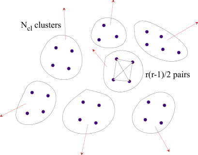
Figure 1: The cluster model of correlations. Particles are grouped in $N_{\rm cl}$ clusters, containing on the average $r$ particles. The particles within a cluster move at very similar collective velocities, indicated by arrows.

Next, we use the experimental fact that the variance of the momentum distribution and its mean are independent of centrality in the fiducial range, which allows us to replace the quantities $\langle p\rangle_{n}$ by $\langle M\rangle$ and $\langle p^{2}\rangle_{n}-\langle p\rangle_{n}^{2}$ by $\sigma_{p}^{2}$ at the average multiplicity, denoted as $\sigma^{2}_{p,\langle n\rangle}$. In this way we get

$$\sigma_{M}^{2}=\sigma_{p,\langle n\rangle}^{2}\sum_{n}\frac{P(n)}{n}+\sum_{n}\frac{P(n)}{n^{2}}\left[\sum_{i,j=1,j\neq i}^{n}{\rm cov}_{n}(p_{i},p_{j})\right].$$ (9)

In the mixed events, by construction, particles are not correlated, hence the covariance term in Eq. (9) vanishes and

$$\sigma_{M}^{2,{\rm mix}}=\sigma_{p,\langle n\rangle}^{2}\sum_{n}\frac{P(n)}{n}\simeq\sigma_{p,\langle n\rangle}^{2}\left(\frac{1}{\langle n\rangle}+\frac{\sigma_{n}^{2}}{\langle n\rangle^{3}}+\dots\right),$$ (10)

where in the last equality we have used the fact that the distribution $P(n)$ is narrow and expanded $1/n=1/[\langle n\rangle+(n-\langle n\rangle)]$ to second order in $(n-\langle n\rangle)$. Comparison made in Table 1 shows that formula (10) works at the 1-2% level. In addition, since $\sigma_{p,\langle n\rangle}$ is not altered by the event mixing procedure, subtracting (10) from (9) yields

$$\sigma_{\rm dyn}^{2}=\sum_{n}\frac{P(n)}{n^{2}}\sum_{i,j=1,j\neq i}^{n}{\rm cov}_{n}(p_{i},p_{j})\simeq\frac{1}{\langle n\rangle^{2}}\sum_{i,j=1,j\neq i}^{\langle n\rangle}{\rm cov}_{\langle n\rangle}(p_{i},p_{j}).$$ (11)

Now we come to the physics discussion. The scaling (3) imposes severe constraints on the physical nature of the covariance term. For instance, if all particles were correlated to each other, $\sum_{i,j=1,j\neq i}^{n}{\rm cov}_{\langle n\rangle}(p_{i},p_{j})$ would be proportional to the number of pairs, and $\sigma_{\rm dyn}$ would not depend on $\langle n\rangle$ at large multiplicities. A natural explanation of the scaling (3) comes from the cluster model, depicted in Fig. 1. The system is assumed to have $N_{\rm cl}$ clusters, each containing (on the average) $r$ particles. Below we keep $r={\rm const.}$ for simplicity. The particles are correlated if and only if they belong to the same cluster, where the covariance per pair is $2\,{\rm cov}^{\ast}$. The number of correlated pairs within a cluster is $r(r-1)/2$. Some particles may be unclustered, hence the ratio of clustered to all particles is $\langle N_{\rm cl}\rangle r/\langle n\rangle=\alpha$. If all particles are clustered then $\alpha=1$. With these assumptions Eq. (11) becomes

$$\sigma_{\rm dyn}^{2}=\frac{\alpha(r-1)}{\langle n\rangle}{\rm cov}^{\ast},$$ (12)

which complies to the scaling (3). An immediate conclusion here is that the ratio $\alpha$ cannot depend on $\langle n\rangle$ (in the fiducial centrality range) in order for the scaling to hold.

The question now is whether we can use the above results to draw conclusions on effects of jets (minijets), which have been proposed as a possible explanation of the experimental data even at the considered soft momenta [20]. Jets, when fragmenting, lead to clusters in the momentum space. The resulting full covariance from jets is then $N_{\rm cl,jet}j(j-1){\rm cov^{j}}/\langle n\rangle^{2}$, where $N_{\rm cl,jet}$ is the number of clusters originating from jets, $j$ is the average number of particles in the cluster, and $2\,{\rm cov^{j}}$ is the average covariance per pair. The total number of particles produced from jets is $N_{\rm cl,jet}j$. On the other hand, the commonly accepted estimate of the dependence of $N_{\rm cl,jet}j$ on centrality is accounted for by the nuclear modification factor $R_{AA}$ multiplied by the number of binary nucleon-nucleon collisions $N_{\rm bin}$. Since $R_{AA}$ depends on the ratio $\langle n\rangle/\langle n\rangle_{pp}$, where $\langle n\rangle_{pp}$ is the multiplicity in the proton-proton collisions, in a given $p_{T}$ bin one finds

$$N_{\rm cl,jet}j\sim R_{AA}N_{\rm bin}=\frac{\langle n\rangle}{N_{\rm bin}\langle n\rangle_{pp}}N_{\rm bin}\sim\langle n\rangle,$$ (13)

which complies to the scaling of Eq. (12). We stress that this scaling follows just from the presence of clusters, and is insensitive to the nature of their physical origin as long as one imposes $N_{\rm cl}\sim\langle n\rangle$. In other words, as long as Eq. (13) is used, the explanation of the observed data in terms of quenched jets agrees with the cluster picture. However, the explanation of the centrality dependence of the $p_{T}$ fluctuations in terms of jets based solely on Eq. (13) is insufficient and not conclusive: any mechanism leading to clusters would do. Microscopic realistic estimates of the magnitude of ${\rm cov^{j}}$ and $j$ are necessary in that regard, including the interplay of jets and medium. For the current status of this program the user is referred to [21, 22].

Before continuing the analysis of the cluster model in a more quantitative manner we need to consider the effects of acceptance and detector efficiency. This is particularly important in the event-by-event analysis, since the experiments select particles with very clearly identified tracks, and thus the detector efficiency, denoted by $a$, is small. The number of observed particles is proportional to $a$, and the number of pairs contributing to the covariance is proportional to $a^{2}$. Thus Eq. (12) may be rewritten as $\sigma_{\rm dyn}^{2}=\frac{r-1}{\langle n\rangle}_{\!\!\!\rm full}{\rm cov}^{\ast}=a\frac{r-1}{\langle n\rangle}_{\!\!\!\rm obs}{\rm cov}^{\ast}$, where ”full” denotes all particles (that would be observed with 100% efficiency), while ”obs” stands for the actually observed multiplicity of particles. Thus

$${\rm cov}^{\ast}=\sigma_{\rm dyn}^{2}\frac{\langle n\rangle_{\!\rm obs}}{a(r-1)}.$$ (14)

Our estimate for $a$ in the PHENIX experiment is of the order of 10%, which together with the numbers of Table 1 gives

$${\rm cov}^{\ast}\simeq\frac{0.035~{}{\rm GeV}^{2}}{(r-1)}.$$ (15)

In the considered problem the coefficient $0.035~{}{\rm GeV}^{2}$ is not a small number when compared to the natural scale set by the variance $\sigma_{p}^{2}\simeq 0.08~{}{\rm GeV}^{2}$. We recall that $\mid{\rm cov}^{\ast}\mid\leq\sigma_{p}^{2}$. Comparing the numbers, we note that for $r=2$ the value of ${\rm cov}^{\ast}$ would assume almost a half of the maximum possible value. This is very unlikely, as argued in the dynamical estimates presented below, which give ${\rm cov}^{\ast}$ at most $0.01~{}{\rm GeV}^{2}$. Thus a natural explanation of the values in (15) is to take a significantly larger value of $r$. Of course, the higher value, the easier it is to satisfy (15) even with small values of ${\rm cov}^{\ast}$. We call this picture the “lumped clusters”: lumps of matter move at some collective velocities, correlating the momenta of particles belonging to the same cluster, see Fig. 1.

The above estimates were based on the PHENIX data [1], however, very similar quantitative conclusions can be reached from the recently published STAR data [3]. We note that the measure $\langle\Delta p_{i}\Delta p_{j}\rangle$ used by STAR is just the estimator for $\sigma_{\rm dyn}^{2}$. Indeed, elementary steps lead to

$$\langle\Delta p_{i}\Delta p_{j}\rangle=\frac{N_{\rm event}-1}{N_{\rm event}}{\sigma}^{2}_{M}-\frac{1}{N_{\rm event}}\sum_{k=1}^{N_{\rm event}}\frac{{\sigma}^{2}_{p}}{N_{k}}.$$ (16)

Comparison to (9) leads immediately for a large number of events to $\langle\Delta p_{i}\Delta p_{j}\rangle=\sigma_{\rm dyn}^{2}$. Now, taking the values of Table I of Ref. [3] and assuming $a=0.75$ we find ${\rm cov}^{\ast}(r-1)=0.058,0.043,0.035,0.014~{}{\rm GeV}^{2}$ for $\sqrt{s_{NN}}=200,130,62$ and 20 GeV, respectively. The value at 130 GeV is close to the value (15). Interestingly, we note a significant beam-energy dependence, with ${\rm cov}^{\ast}(r-1)$ increasing with $\sqrt{s_{NN}}$. This may be due to the increase of the covariance per correlated pair with the increasing energy, and/or an increase of the number of clustered particles.

In the last part of this paper we present some dynamical estimates of ${\rm cov}^{\ast}$ in thermal models. The first calculation concerns the role of resonances in $p_{T}$ correlations. Clearly, a resonance, such as the $\rho$ meson, decaying into daughter particles induces momentum correlations. We make a numerical calculation of this effect in the model of Ref. [23, 24], using the formula

$${\rm cov}^{\ast}_{\rm res}={\!\int\!d^{3}p\!\int{d^{3}p_{1}\over E_{p_{1}}}\!\int{d^{3}p_{2}\over E_{p_{2}}}\,\delta^{(4)}(p-p_{1}-p_{2})C{dN_{R}\over d^{3}p}\left(p_{1}^{\perp}\!-\!\langle p^{\perp}\rangle\right)\left(p_{2}^{\perp}\!-\!\langle p^{\perp}\rangle\right)\over\!\int\!d^{3}p\int{d^{3}p_{1}\over E_{p_{1}}}\int{d^{3}p_{2}\over E_{p_{2}}}\,\delta^{(4)}(p-p_{1}-p_{2})C{dN_{R}\over d^{3}p}},$$ (17)

where $dN_{R}/d^{3}p$ is the resonance distribution in the momentum space (obtained from the Cooper-Frye formula as described in Ref. [25]), $p_{1}$ and $p_{2}$ are the momenta of the emitted particles, $E_{p}$ is the energy of a particle with momentum $p$, and the function $C$ represents the experimental cuts. We note that from now on the letter $p$, depending on the context, denotes the four- or three-momentum. The results of our numerical study show that for the resonance mass between 500 MeV and 1.2 GeV the covariance ${\rm cov}^{\ast}_{\rm res}$ varies between 0.005 GeV² at low masses to $-0.015$ GeV² at high masses, changing sign around 700-800 MeV, depending on the assumed experimental cuts. Thus, cancellations between contributions of various resonances are possible; in fact, a full-fledged simulation with Therminator [26] revealed a negligible contribution of resonances to the $p_{T}$ correlations. Of course, the “lumpy” feature of the expansion was not implemented in the calculation. Details of this study will be presented elsewhere.

The second model of particle correlations assumes that the particle emission at the lowest scales occurs from local thermalized sources. Each element of the fluid moves with its collective velocity and emits particles with locally thermalized spectra. This picture was put forward as a mechanism creating correlations in the charge balance function [25, 27] resulting from charge conservation within the local source. Correlations between particles emitted from the same cluster come from the fact that those particles are emitted from a source with the same collective transverse velocity. The average number of particles $r$ originating from such a local source determines the strength of the surviving dynamical fluctuation in the whole event, as discussed above. The covariance between particles $i$ and $j$ emitted from a cluster moving with a velocity $u$ is

$${\rm cov}^{\ast}(i,j)=\frac{\int d\Sigma_{\mu}u^{\mu}\int d^{3}p_{1}(p^{\perp}_{1}-\langle p^{\perp}\rangle)f_{i}^{u}(p_{1})\int d^{3}p_{2}(p^{\perp}_{2}-\langle p^{\perp}\rangle)f_{j}^{u}(p_{2})}{\int d\Sigma_{\mu}u^{\mu}\int d^{3}p_{1}f_{i}^{u}(p_{1})\int d^{3}p_{2}f_{j}^{u}(p_{2})},$$ (18)

where $f_{i}^{u}(p)=(\exp(p\cdot u/T)\pm 1)^{-1}$ is the boosted thermal distribution and $d\Sigma_{\mu}$ denotes integration over the freeze-out hypersurface. The result turns out to depend strongly on the temperature. Considering the emission of correlated pion pairs one gets ${\rm cov}^{\ast}(\pi,\pi)=0.0034~{}{\rm GeV}^{2}$ for freeze-out parameters corresponding to the single freeze-out model [23]($T=165$ MeV, average flow velocity $0.5c$) and ${\rm cov}^{\ast}(\pi,\pi)=0.01~{}{\rm GeV}^{2}$ for parameters corresponding to a late kinetic freeze-out ($T=100$ MeV, average flow velocity $0.6c$). For realistic values of thermal freeze-out parameters the experimentally estimated value of the covariance cannot be accounted for, unless the number of charged particles belonging to the same cluster is at least $4-10$.

In conclusion, we have found that in the fiducial centrality range the scaling of the $\sigma_{\rm dyn}^{2}$ for the $p_{T}$ correlations with inverse particle multiplicity indicates the cluster nature of the system formed in relativistic heavy-ion collisions. The clusters may a priori originate from very different physics: jets, droplets of fluid formed in the explosive scenario of the collision, or other mechanisms leading to multiparticle correlations. A larger number of particles within a cluster helps to obtain the large measured value of $\sigma_{\rm dyn}^{2}$.

References

• [1] PHENIX, K. Adcox etΒ al., Phys. Rev. C66 (2002) 024901, nucl-ex/0203015.
• [2] STAR, J. Adams etΒ al., Phys. Rev. C71 (2005) 064906, nucl-ex/0308033.
• [3] STAR, J. Adams etΒ al., (2005), nucl-ex/0504031.
• [4] M. Gazdzicki and S. Mrowczynski, Z. Phys. C54 (1992) 127.
• [5] L. Stodolsky, Phys. Rev. Lett. 75 (1995) 1044.
• [6] E.V. Shuryak, Phys. Lett. B423 (1998) 9, hep-ph/9704456.
• [7] S. Mrowczynski, Phys. Lett. B430 (1998) 9, nucl-th/9712030.
• [8] M.A. Stephanov, K. Rajagopal and E.V. Shuryak, Phys. Rev. D60 (1999) 114028, hep-ph/9903292.
• [9] S.A. Voloshin, V. Koch and H.G. Ritter, Phys. Rev. C60 (1999) 024901, nucl-th/9903060.
• [10] NA49, H. Appelshauser etΒ al., Phys. Lett. B459 (1999) 679, hep-ex/9904014.
• [11] R. Korus etΒ al., Phys. Rev. C64 (2001) 054908, nucl-th/0106041.
• [12] G. Baym and H. Heiselberg, Phys. Lett. B469 (1999) 7, nucl-th/9905022.
• [13] A. Bialas and V. Koch, Phys. Lett. B456 (1999) 1, nucl-th/9902063.
• [14] M. Asakawa, U.W. Heinz and B. Muller, Phys. Rev. Lett. 85 (2000) 2072, hep-ph/0003169.
• [15] H. Heiselberg, Phys. Rept. 351 (2001) 161, nucl-th/0003046.
• [16] C. Pruneau, S. Gavin and S. Voloshin, Phys. Rev. C66 (2002) 044904, nucl-ex/0204011.
• [17] S. Jeon and V. Koch, in Quark-Gluon Plasma 3, eds. R.Β C.Β Hwa and X.Β N.Β Wang, p.Β 430, World Scientific Singapore (2004), hep-ph/0304012.
• [18] S. Gavin, Phys. Rev. Lett. 92 (2004) 162301, nucl-th/0308067.
• [19] M. Abdel-Aziz and S. Gavin, (2005), nucl-th/0510011.
• [20] PHENIX, S.S. Adler etΒ al., Phys. Rev. Lett. 93 (2004) 092301, nucl-ex/0310005.
• [21] Q.J.Β Liu and T.A. Trainor, Phys. Lett. B567 (2003) 184, hep-ph/0301214.
• [22] J.T. Mitchell, talk at ”Workshop on Correlations and Fluctuations in Relativistic Nuclear Collisions”, MIT, 21-23 April 2005,
Β http://www.mit.edu/Β vaurynov/21april2005workshop.
• [23] W. Broniowski and W. Florkowski, Phys. Rev. Lett. 87 (2001) 272302, nucl-th/0106050.
• [24] W. Broniowski, A. Baran and W. Florkowski, Acta Phys. Polon. B33 (2002) 4235, hep-ph/0209286.
• [25] P. Bozek, W. Broniowski and W. Florkowski, Acta Phys. Hung. A22 (2005) 149, nucl-th/0310062.
• [26] A. Kisiel etΒ al., (2005), nucl-th/0504047.
• [27] S. Cheng etΒ al., Phys. Rev. C69 (2004) 054906, nucl-th/0401008.