Particle Number Fluctuations in Relativistic Bose and Fermi Gases

Abstract

Particle number fluctuations are studied in relativistic Bose and Fermi gases. The calculations are done within both the grand canonical and canonical ensemble. The fluctuations in the canonical ensemble are found to be different from those in the grand canonical one. Effects of quantum statistics increase in the grand canonical ensemble for large chemical potential. This is, however, not the case in the canonical ensemble. In the limit of large charge density a strongest difference between the grand canonical and canonical ensemble results is observed.

I Introduction

The statistical models have been successfully used to describe the data on hadron multiplicities in relativistic nucleus-nucleus (A+A) collisions (see, e.g., Ref. stat-model and recent review BMST ). This has stimulated an investigation of the properties of these statistical models. In particular, connections between different statistical ensembles for a system of relativistic particles have been intensively discussed. In A+A collisions one prefers to use the grand canonical ensemble (GCE) because it is the most convenient one from the technical point of view. The canonical ensemble (CE) ce-a ; ce ; ce-b ; ce-c ; ce-d ; ce-e or even the microcanonical ensemble (MCE) mce have been used in order to describe the $pp$, $p\bar{p}$ and $e^{+}e^{-}$ collisions when a small number of secondary particles are produced. At these conditions the statistical systems are far away from the thermodynamic limit, so that the statistical ensembles are not equivalent, and the exact charge or both energy and charge conservation laws have to be taken into account. The CE suppression effects for particle multiplicities are well known in the statistical approach to hadron production, e.g., the suppression in a production of strange hadrons ce-c and antibaryons ce-d in small systems, i.e., when the total numbers of strange particles or antibaryons are small (smaller than or equal to 1). The different statistical ensembles are not equivalent for small systems. When the system volume increases, $V\rightarrow\infty$, the average quantities in the GCE, CE and MCE become equal, i.e., all ensembles are thermodynamically equivalent.

The situation is different for the statistical fluctuations. The fluctuations in relativistic systems are studied in event by event analysis of high energy particle and nuclear collisions (see, e.g., Refs.  fluc ; step ; step1 ; fluc1 and references therein). In the relativistic system of created particles, only the net charge $Q=N_{+}-N_{-}$ (e.g., electric charge, baryonic number, and strangeness) can be fixed. In the statistical equilibrium an average value of the net charge is fixed in the GCE, or exact one in the CE, but $N_{+}$ and $N_{-}$ numbers fluctuate in both GCE and CE.

The particle number fluctuations for the relativistic case in the CE were calculated for the first time in Ref. ce-fluc for the Boltzmann ideal gas with net charge equal to zero. These results were then extended for the CE ce2-fluc ; ce3-fluc ; bec and MCE mce-fluc ; mce2-fluc and compared with the corresponding results in the GCE (see also Ref. turko ). The particle number fluctuations have been found to be suppressed in the CE and MCE in a comparison with the GCE. This suppression survives in the limit $V\rightarrow\infty$, so that the thermodynamical equivalence of all statistical ensembles refers to the average quantities, but does not apply to the fluctuations.

In the present paper we study the particle number fluctuations in relativistic ideal Bose and Fermi gases for non-zero values of the net charge density in the GCE and CE. The paper is organized as follows. In Sections II and III we calculate the average values for $N_{+}$ and $N_{-}$ and discuss the Bose condensation in relativistic gases. These results are not new, and we present them in our paper for completeness. In Section IV we consider the $N_{+}$ and $N_{-}$ fluctuations in the GCE and study the Bose and Fermi effects for particle number densities. In Section V the same calculations and study are repeated within the CE. We compare the GCE and CE results and summarize our consideration in Section VI.

II Average particle numbers

The relativistic ideal Bose or Fermi gas can be characterized by the occupation numbers $n_{p}^{+}$ and $n_{p}^{-}$ of the one-particle states labeled by momenta $p$ for ’positively charged’ particles and ’negatively charged’ particles, respectively. The GCE average values are lan :

$$\langle n_{p}^{\pm}\rangle_{g.c.e.}~{}=~{}\frac{1}{\exp\left[\left(\sqrt{p^{2}+m^{2}}~{}\mp~{}\mu\right)/T\right]~{}-~{}\gamma}~{},$$ (1)

where $m$ is the particle mass, $T$ is the system temperature and $\mu$ is the chemical potential connected with the conserved charge $Q$:

$$Q~{}\equiv~{}\langle N_{+}\rangle_{g.c.e.}~{}-~{}\langle N_{-}\rangle_{g.c.e.}~{}=~{}\sum_{p}\langle n_{p}^{+}\rangle_{g.c.e.}~{}-~{}\sum_{p}\langle n_{p}^{-}\rangle_{g.c.e.}~{}.$$ (2)

The parameter $\gamma$ in Eq. (1) is equal to $+1$ and $-1$ for Bose and Fermi statistics, respectively ($\gamma=0$ corresponds to the Boltzmann approximation). Each level should be further specified by the projection of a particle spin. Thus, each $p$-level splits into $g=2j+1$ sub-levels. It will be assumed that the $p$-summation includes all these sub-levels too. In the thermodynamic limit the system volume $V$ goes to infinity, and the degeneracy factor $g$ enters explicitly when one substitutes the summation over discrete levels by the integration, $\sum_{p}~{}...~{}=~{}gV(2\pi^{2})^{-1}~{}\int_{0}^{\infty}p^{2}dp~{}...~{}$. The particle number densities in the GCE are:

$$\rho_{\pm} \;\equiv~{}\frac{\langle N_{\pm}\rangle_{g.c.e.}}{V}~{}=~{}\frac{\sum_{p}\langle n^{\pm}_{p}\rangle_{g.c.e.}}{V}\;=\;\frac{g}{2\pi^{2}}\;\int_{0}^{\infty}\frac{p^{2}dp}{\exp\left[\left(\sqrt{p^{2}+m^{2}}~{}\mp~{}\mu\right)/T\right]~{}-~{}\gamma}$$

$$\;=\;\frac{g\,T^{3}}{2\pi^{2}}\;\int_{0}^{\infty}\frac{x^{2}dx}{\exp\left[\sqrt{x^{2}+m^{*\,2}}~{}\mp~{}\mu^{*}\right]~{}-~{}\gamma}\;,$$ (3)

where $m^{*}\equiv m/T,\;\mu^{*}\equiv\mu^{*}/T\;$. To be definite we consider $\mu^{*}\geq 0$ in what follows. This corresponds to non-negative values of the system charge density $\rho_{Q}\equiv\rho_{+}-\rho_{-}\geq 0$. Results for $\mu^{*}\leq 0$ can be obtained from those with $\mu^{*}\geq 0$ by exchanging of $N_{+}$ and $N_{-}$. In the Boltzmann approximation ($\gamma=0$) one finds:

$$\rho_{\pm}^{Boltz}\;=\;\frac{g\,T^{3}}{2\pi^{2}}\;m^{*\,2}\,K_{2}(m^{*})\,\exp(\pm\mu^{*})\;\simeq\;\begin{cases}g\,T^{3}\;\exp(\pm\mu^{*})/\pi^{2}\;,\quad&m^{*}\ll 1\vspace{0.2cm}\\ \;g\,T^{3}\,(m^{*}/2\pi)^{3/2}\;\exp[-(m^{*}\mp\mu^{*})]\;,\quad&m^{*}\gg 1\end{cases}$$ (4)

where $\;K_{2}\;$ is a modified Hankel function. For $0\leq\mu^{*}\leq m^{*}$ it follows from Eq. (II):

$$\rho_{\pm}\;=\;\frac{g\,T^{3}}{2\pi^{2}}\;m^{*\,2}\,\sum_{n=1}^{\infty}\frac{\gamma^{n-1}}{n}\;K_{2}(nm^{*})\,\exp(\pm n\mu^{*})~{}.$$ (5)

Note that for $\rho_{-}^{Fermi}$ the series expansion in Eq. (5) is convergent for all $\mu^{*}$. The first term, $n=1$, in Eq. (5) corresponds to the Boltzmann approximation and others, $n>1$, are the Bose ($\gamma=1$) or Fermi ($\gamma=-1$) statistics corrections. For any $T$ and $\mu$ these correction terms lead to $\rho_{\pm}^{Bose}>\rho_{\pm}^{Boltz}$ and $\rho_{\pm}^{Fermi}<\rho_{\pm}^{Boltz}$ for the particle number densities. The Bose enhancement and Fermi suppression factors,

$$R_{\pm}^{Bose}~{}\equiv~{}\frac{\rho_{\pm}^{Bose}}{\rho_{\pm}^{Boltz}}~{},~{}~{}~{}~{}R_{\pm}^{Fermi}~{}\equiv~{}\frac{\rho_{\pm}^{Fermi}}{\rho_{\pm}^{Boltz}}~{},$$ (6)

for different values of $m^{*}$ are shown in Fig. 1 as functions of $\mu^{*}$.

Figure 1: The ratios $R_{+}$ (left) and $R_{-}$ (right) of particle number densities of bosons ($\gamma=1$) and fermions ($\gamma=-1$) to those of classical particles ($\gamma=0$) are shown as functions of $\mu^{*}$. Two upper solid lines show $R_{\pm}^{Bose}$ at $m^{*}=1,~{}3$. Three lower solid lines show $R_{\pm}^{Fermi}$ at $m^{*}=0,~{}1,~{}3$. The vertical dotted lines $\mu^{*}=1,~{}3$ demonstrate the restriction $\mu^{*}\leq m^{*}$ in the Bose gas. The crosses at the end of the $R_{+}^{Bose}$ and $R_{-}^{Bose}$ lines at $\mu^{*}=1$ and $\mu^{*}=3$ correspond to the points of the Bose condensation. The crosses at $\mu^{*}=0$ correspond to the limit $m^{*}\rightarrow 0$ given by Eq. (7) in the Bose gas. The dashed horizontal line on the left corresponds to the maximum value for $R_{+}^{Bose}$ given by Eq. (10).

One finds that the largest quantum statistics effects at $\mu^{*}=0$ correspond to the massless particles:

$$R_{\pm}^{Bose}(\mu^{*}=0,~{}m^{*}\rightarrow 0)~{} =~{}\frac{1}{2}\int_{0}^{\infty}\frac{x^{2}dx}{\exp(x)~{}-~{}1}~{}=~{}\sum_{n=1}^{\infty}\frac{1}{n^{3}}~{}=~{}\zeta(3)\simeq 1.202~{},$$ (7)

$$R_{\pm}^{Fermi}(\mu^{*}=m^{*}=0)~{} =~{}\frac{1}{2}\int_{0}^{\infty}\frac{x^{2}dx}{\exp(x)~{}+~{}1}~{}=~{}\sum_{n=1}^{\infty}\frac{(-1)^{n+1}}{n^{3}}~{}=~{}\frac{3}{4}\,\zeta(3)\simeq 0.902~{},$$ (8)

where $\zeta(k)$ is a Riemann zeta function (see Appendix A). Note that the values of $n_{0}^{+}$ and $n_{0}^{-}$ contribute to the net charge of the system, but for $m=0$ they do not influence the system energy. Therefore, the occupation numbers $n_{0}^{+}$ and $n_{0}^{-}$ become arbitrary, and the ideal Bose gas of charge particles with $m=0$ has no clear meaning in the thermodynamic limit. In what follows the ’massless’ Bose gas of charged particles will be understood as the limit $m^{*}\rightarrow 0$ at fixed value of $\mu^{*}\equiv 0$.

For $m^{*}\gg 1$ using the asymptotic of the $K_{2}$ function one finds:

$$\rho_{\pm}~{}\simeq~{}\frac{g\,T^{3}\,m^{*\,3/2}}{(2\pi)^{3/2}}\,\sum_{n=1}^{\infty}\frac{(\gamma)^{n-1}}{n^{3/2}}~{}\exp\left[-n\,(m^{*}~{}\mp~{}\mu^{*})\right]\;=\;\frac{g\,T^{3}\,m^{*\,3/2}}{(2\pi)^{3/2}}~{}\gamma~{}Li_{3/2}(\gamma\exp[-(m^{*}~{}\mp~{}\mu^{*})])$$ (9)

where $\sum_{n=1}^{\infty}z^{n}/n^{k}=Li_{k}(z)$, is a polylogarithm function (see Appendix A). For $\;z=1\;$ it equals to the Riemann zeta function, $\;Li_{k}(1)=\zeta(k)\;$. The series expansion in Eq. (9) for $\rho_{+}$ converges rapidly at $\mu^{*}\ll m^{*}$. In this case it is enough to add one term $n=2$ to the Boltzmann approximation ($n=1$) to describe accurately the Bose or Fermi effects. The same is valid for $\rho_{-}$ at $m^{*}\gg 1$ for all $\mu^{*}$.

The condition $\mu^{*}\leq m^{*}$ is a general requirement in the Bose gas. At $\mu^{*}\rightarrow m^{*}$ the Bose enhancement factor $R_{+}^{Bose}$ reaches its maximum value, and the Bose condensation of positively charged particles starts. This maximum value of $R_{+}^{Bose}$ at $\mu^{*}=m^{*}$ increases with $m^{*}$ and reaches its upper limit,

$$max[R_{+}^{Bose}(\mu^{*},m^{*})]~{}=~{}R_{+}^{Bose}(\mu^{*}=m^{*}\rightarrow\infty)~{}=~{}Li_{3/2}(1)~{}=~{}\zeta(3/2)~{}\simeq 2.612~{},$$ (10)

at $m^{*}\rightarrow\infty$ (see Fig. 1, left). For negatively charged particles the Bose enhancement factor reaches its minimal value at $\mu^{*}=m^{*}$,

$$R_{-}^{Bose}(\mu^{*}=m^{*})~{}\simeq~{}1~{}+~{}\frac{K_{2}(2m^{*})}{2K_{2}(m^{*})}~{}\exp\left(-m^{*}\right),$$ (11)

and this value goes to 1 (i.e. to its classical Boltzmann limit) from above at $m^{*}\rightarrow\infty$ (see Fig. 1, right).

The requirement $\mu^{*}\leq m^{*}$ is absent for the Fermi gas and for $\mu\gg m$ one finds (see Eq. (B) in Appendix B):

$$\rho_{+}^{Fermi}~{}\simeq~{}\frac{g\,T^{3}}{2\pi^{2}}\,\left[\;\frac{1}{3}\;\mu^{*\,3}+\left(\frac{\pi^{2}}{3}-\frac{m^{*\,2}}{2}\right)\mu^{*}\right]\,,$$ (12)

while the density for negatively charged particles can be approximated in this limit with the first two terms from the right-hand side of Eq. (5): $n=1$ corresponds to the Boltzmann approximation $\rho_{-}^{Boltz}$  (4), and $n=2$ gives a small (negative) Fermi correction. Thus, one finds that $R_{+}^{Fermi}$ goes to zero (see Fig. 1, left) and $R_{-}^{Fermi}$ goes to 1 from below (see Fig. 1, right) at $\mu^{*}\rightarrow\infty$:

$$R_{+}^{Fermi}~{}\simeq~{}\frac{\mu^{*3}\,\exp\left(-\mu^{*}\right)}{3~{}m^{*2}K_{2}(m^{*})}~{}\rightarrow~{}0~{},~{}~{}~{}~{}R_{-}^{Fermi}~{}\simeq~{}1~{}-~{}\frac{K_{2}(2m^{*})}{2K_{2}(m^{*})}~{}\exp\left(-\mu^{*}\right)\rightarrow~{}1~{}.$$ (13)

III Bose condensation

In a standard non-relativistic picture of the Bose condensation the particle number $N$ is a conserved quantity. If the system temperature decreases at fixed particle number density $\rho=N/V$, the system chemical potential increases and reaches its maximal value at $T=T_{C}$. Bose condensation starts and a macroscopic part of the system particles – known as the Bose condensate – occupies the lowest momentum state at $T<T_{C}$. In a relativistic picture the conserved quantity is system charge $Q=N_{+}-N_{-}$. From Eq. (5) one finds for the dimensionless charge density:

$$\widetilde{\rho}_{Q}~{}\equiv~{}\frac{\rho_{Q}}{g\,m^{3}}~{}\equiv~{}\frac{1}{g\,m^{3}}~{}\left(\rho_{+}^{Bose}~{}-~{}\rho_{-}^{Bose}\right)\;=\;\frac{1}{\pi^{2}}~{}\sum_{n=1}^{\infty}\frac{1}{n\,m^{*}}~{}\;K_{2}\left(n\,m^{*}\right)~{}\sinh(n\,\mu^{*})~{}.$$ (14)

Bose condensation starts at the point $\;T=T_{C}\;$ when $\;\mu=\mu^{max}=m\;$. At this point Eq. (14) is reduced to:

$$\widetilde{\rho}_{Q}~{}=~{}\frac{\widetilde{T}_{C}}{\pi^{2}}~{}\sum_{n=1}^{\infty}\frac{1}{n}\;K_{2}\left(n/\widetilde{T}_{C}\right)~{}\sinh(n/\widetilde{T}_{C})~{},$$ (15)

where $\widetilde{T}_{C}\equiv T_{C}/m$. Equation (15) can be used to write the Bose condensation temperature $T_{C}$ as the function of the conserved charge density $\rho_{Q}$. The line of Bose condensation $\widetilde{T}_{C}=\widetilde{T}_{C}(\widetilde{\rho}_{Q})$ given by Eq. (15) is shown in Fig. 2 (see also Ref. TC and references therein).

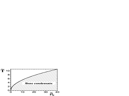
Figure 2: The phase diagram of the relativistic ideal Bose gas. The solid line shows Bose condensation temperature as a function of the conserved charge density. It is given by Eq.(15) where both quantities are expressed in dimensionless form: $\widetilde{T}_{C}\equiv T_{C}/m,~{}\widetilde{\rho}_{Q}\equiv\rho_{Q}/(gm^{3})$. At $\widetilde{T}_{C}\ll 1$ the line $\widetilde{T}_{C}(\widetilde{\rho}_{Q})$ is given by non-relativistic approximation (16), while at $\widetilde{T}_{C}\gg 1$ it is described by the ultra-relativistic relation (17). The points $(\widetilde{\rho}_{Q},\widetilde{T})$ under the solid line correspond to the states of the system with non-zero values of the Bose condensate.

At $\widetilde{T}_{C}\ll 1$ it follows from Eq. (15):

$$\widetilde{\rho}_{Q}\;\simeq\;\left(\frac{\widetilde{T}_{C}}{2\pi}\right)^{3/2}\sum_{n=1}^{\infty}\frac{1}{n^{3/2}}\;=\;\left(\frac{\widetilde{T}_{C}}{2\pi}\right)^{3/2}\,\zeta(3/2)~{}.$$ (16)

This corresponds to a non-relativistic limit. The density of negatively charged particles at $T\simeq T_{C}$ behaves as $\rho_{-}\propto\exp(-2/\widetilde{T}_{C})$ and can be neglected in a comparison with $\rho_{+}\propto(\widetilde{T}_{C})^{3/2}$. Under these conditions the charge number conservation becomes equivalent just to the (positively charged) particle number conservation. One, therefore, recovers from Eq. (16) the familiar relation, $\widetilde{T}_{C}\simeq 3.313\widetilde{\rho}_{Q}^{~{}2/3}$, between the Bose condensation temperature and particle number density known in the non-relativistic statistical mechanics lan . At $\widetilde{T}_{C}\gg 1$ from Eq. (15) one finds:

$$\widetilde{\rho}_{Q}\;\simeq\;\frac{2\,\widetilde{T}_{C}^{2}}{\pi^{2}}\sum_{n=1}^{\infty}\frac{1}{n^{2}}\;=\;\frac{\widetilde{T}_{C}^{2}}{3}~{}.$$ (17)

This corresponds to the ultra-relativistic limit and leads to a new relation, $\widetilde{T}_{C}\simeq 1.732\widetilde{\rho}_{Q}^{~{}1/2}$, between the Bose condensation temperature and charge number density.

For fixed value of the conserved charge density $\rho_{Q}$ the chemical potential is constant $\mu^{*}=m^{*}$ at $T\leq T_{C}$. The positively charged particles have to condensate at the lowest quantum level to preserve a constant value of the positive charge density in the system. Therefore, one finds at $T\leq T_{C}$:

$$\rho_{Q}~{}=~{}\rho_{+}^{Bose}(T,\mu^{*}=m^{*})~{}-~{}\rho_{-}^{Bose}(T,\mu^{*}=m^{*})~{}+~{}\rho_{+}^{cond}(T)~{},$$ (18)

where the first two terms in Eq. (18) are given by Eq. (II), and $\rho_{+}^{cond}$ is the density of positively charged particles at the lowest quantum level (Bose condensate). The behavior of $\rho_{+}^{Bose}$, $\rho_{-}^{Bose}$ and $\rho_{+}^{cond}$ above and below the Bose condensation temperature are shown in Fig. 3. Note that $\rho_{+}^{Bose}$ and $\rho_{-}^{Bose}$ are calculated by Eq. (II) with $\mu^{*}\leq m^{*}$ at $T\geq T_{C}$ (the value of $\mu^{*}$ is defined by the equation $\rho_{Q}=\rho_{+}^{Bose}-\rho_{-}^{Bose}$) and with $\mu^{*}=m^{*}$ at $T<T_{C}$ ($\rho_{+}^{cond}$ is given by Eq. (18) at $T<T_{C}$ and it equals to zero at $T>T_{C}$). The Bose condensation is the 3^rd order phase transition with a maximum of specific heat at $T=T_{C}$.

Figure 3: The solid lines show the ratios $\rho_{+}^{Bose}/\rho_{Q}$, $\rho_{-}^{Bose}/\rho_{Q}$, and $\rho_{+}^{cond}/\rho_{Q}$ as functions on $T/T_{C}$ at fixed values of $\rho_{Q}$ for the relativistic ideal Bose gas. The left and right pictures correspond to the values $\widetilde{T}_{C}=0.5,~{}\widetilde{\rho}_{Q}\simeq 0.06$, and $\widetilde{T}_{C}=10,~{}\widetilde{\rho}_{Q}\simeq 33.3$, respectively. Both these $(\widetilde{\rho}_{Q},\widetilde{T}_{C})$ points belong to the Bose condensation line in Fig. 2 – the first point lies close to the lower left corner and the second point lies close to the upper right corner in Fig. 2. The system presented in the left picture can be treated within non-relativistic approximation. In this case, $\rho_{Q}\simeq\rho_{+}^{Bose}$ and $\rho_{-}^{Bose}/\rho_{+}^{Bose}\ll 1$, so that negatively charged particles can be neglected at $T<T_{C}$ and charge conservation becomes equivalent to particle number conservation. The system presented in the right picture demonstrates the Bose condensation in the ultra-relativistic case: both $\rho+^{Bose}$ and $\rho_{-}^{Bose}$ are essentially larger than conserved charge density $\rho_{Q}$ in the vicinity of the Bose condensation temperature $T=T_{C}$.

IV Particle number fluctuations in the GCE

The GCE fluctuations of the single-mode occupation numbers are equal to lan :

$$\langle\Delta n_{p}^{\pm 2}\rangle_{g.c.e.}\equiv\langle\left(n_{p}^{\pm}-\langle n_{p}^{\pm}\rangle_{g.c.e.}\right)^{2}\rangle_{g.c.e.}~{}=~{}\langle n_{p}^{\pm~{}2}\rangle_{g.c.e.}~{}-~{}\langle n_{p}^{\pm}\rangle^{2}_{g.c.e.}~{}=~{}\langle n_{p}^{\pm}\rangle_{g.c.e.}\left(1+\gamma\langle n_{p}^{\pm}\rangle_{g.c.e.}\right)~{}\equiv~{}v^{\pm~{}2}_{p}~{}.$$ (19)

The fluctuations of the macroscopic observables can be written in terms of the microscopic correlator $\langle\Delta n_{p}^{\alpha}\Delta n_{k}^{\beta}\rangle_{g.c.e.}$, where $\alpha,\beta$ are $+$ and/or $-$, which has a simple form,

$$\langle\Delta n_{p}^{\alpha}\Delta n_{k}^{\beta}\rangle_{g.c.e.}~{}=~{}v_{p}^{\alpha~{}2}~{}\delta_{p\,k}~{}\delta_{\alpha\beta}~{},$$ (20)

due to the statistical independence of different quantum levels and different charge states in the GCE. The variances of the total number of positively and/or negatively charged particles are equal to:

$$\langle\Delta N_{\pm}^{2}\rangle_{g.c.e.}\,\equiv\,\langle N_{\pm}^{2}\rangle_{g.c.e.}-\langle N_{\pm}\rangle^{2}_{g.c.e.}\,=\,\sum_{p,k}\langle n_{p}^{\pm}n_{k}^{\pm}\rangle_{g.c.e.}-\langle n_{p}^{\pm}\rangle_{g.c.e.}\langle n_{k}^{\pm}\rangle_{g.c.e.}=\sum_{p,k}\langle\Delta n_{p}^{\pm}\Delta_{k}^{\pm}\rangle_{g.c.e.}\,=\,\sum_{p}v_{p}^{\pm~{}2}~{}.$$ (21)

The scaled variance $\omega^{\pm}_{g.c.e.}$ reads:

$$\omega^{\pm}_{g.c.e.}~{} \equiv~{}\frac{\langle N_{\pm}^{2}\rangle_{g.c.e.}~{}-~{}\langle N_{\pm}\rangle^{2}_{g.c.e.}}{\langle N_{\pm}\rangle_{g.c.e.}}~{}=~{}\frac{\sum_{p,k}\langle\Delta n_{p}^{\pm}\Delta n_{k}^{\pm}\rangle_{g.c.e.}}{\sum_{p}\langle n^{\pm}_{p}\rangle_{g.c.e.}}~{}=~{}\frac{\sum_{p}v_{p}^{\pm~{}2}}{V~{}\rho_{\pm}}$$

$$=~{}1\;+\;\gamma\;\int_{0}^{\infty}\frac{x^{2}dx}{\left[\;\exp\left(\sqrt{x^{2}+m^{*\,2}}~{}\mp~{}\mu^{*}\right)~{}-~{}\gamma\;\right]^{2}}~{}\times~{}\left[\int_{0}^{\infty}\frac{x^{2}dx}{\;\exp\left(\sqrt{x^{2}+m^{*\,2}}~{}\mp~{}\mu^{*}\right)~{}-~{}\gamma}\right]^{-1}~{},$$ (22)

where the thermodynamic limit is assumed, and the $p$-summation is substituted by the integration similar to Eq. (II). The scaled variances $\omega_{g.c.e.}^{\pm Bose}$ and $\omega_{g.c.e.}^{\pm Fermi}$ for different values of $m^{*}$ are shown in Fig. 4 as functions of $\mu^{*}$.

Figure 4: The scaled variances $\omega_{g.c.e.}^{+}$ (left) and $\omega_{g.c.e.}^{-}$ (right) given by Eq. (IV) for bosons ($\gamma=1$) and fermions ($\gamma=-1$) are shown as functions of $\mu^{*}$. The two upper solid lines present $\omega_{g.c.e.}^{\pm Bose}$ for $m^{*}=1,~{}3$. The three lower solid lines present $\omega_{g.c.e.}^{\pm Fermi}$ for $m^{*}=0,~{}1,~{}3$. The vertical dotted lines $\mu^{*}=1,~{}3$ demonstrate the restriction $\mu^{*}\leq m^{*}$ in the Bose gas. The crosses at the end of the lines for $\omega_{g.c.e.}^{-Bose}$ at $\mu^{*}=1$ and $\mu^{*}=3$ correspond to the points of the Bose condensation, $\omega_{g.c.e.}^{+Bose}$ diverges at these points. The crosses at $\mu^{*}=0$ correspond to the limit $m^{*}\rightarrow 0$ given by Eq. (24) in the Bose gas.

It follows from Eq. (IV) for $\gamma=0$,

$$\omega^{+~{}Boltz}_{g.c.e.}~{}=~{}\omega^{-~{}Boltz}_{g.c.e.}~{}=~{}1~{},$$ (23)

i.e. the scaled variances for Boltzmann statistics in the GCE are independent of the chemical potential $\mu^{*}$ and equal to 1 for both the positively and negatively charged particles. The Eq. (IV) leads to the Bose enhancement, $\omega_{g.c.e.}^{\alpha~{}Bose}>1$, and the Fermi suppression $\omega_{g.c.e.}^{\alpha~{}Fermi}<1$, of the particle number fluctuations.

At $\mu^{*}=0$ the largest Bose and Fermi effects correspond to the massless particles (see Fig. 4):

$$\omega^{\pm~{}Bose}_{g.c.e}(\mu^{*}=0,~{}m^{*}\rightarrow 0)~{} =~{}1~{}+~{}\int_{0}^{\infty}\frac{x^{2}dx}{\left[\;\exp(x)~{}-~{}1\;\right]^{2}}~{}\times~{}\left[\int_{0}^{\infty}\frac{x^{2}dx}{\exp(x)~{}-~{}1}\right]^{-1}~{}=~{}\frac{\zeta(2)}{\zeta(3)}~{}\simeq~{}1.368~{},$$ (24)

$$\omega^{\pm~{}Fermi}_{g.c.e}(\mu^{*}=m^{*}=0)~{} =~{}1~{}-~{}\int_{0}^{\infty}\frac{x^{2}dx}{\left[\;\exp(x)~{}+~{}1\;\right]^{2}}~{}\times~{}\left[\int_{0}^{\infty}\frac{x^{2}dx}{\exp(x)~{}+~{}1}\right]^{-1}~{}=~{}\frac{2}{3}\;\frac{\zeta(2)}{\zeta(3)}~{}\simeq~{}0.912~{},$$ (25)

Using Eqs. (54-55) one finds from Eq. (IV) at $\mu^{*}\leq m^{*}$:

$$\omega_{g.c.e.}^{\pm}~{}=~{}1~{}+~{}\gamma~{}\sum_{n=1}^{\infty}\frac{\gamma^{n-1}~{}n}{n+1}\;K_{2}\left[(n+1)\,m^{*}\right]\,\exp\left[\pm~{}(n+1)\,\mu^{*}\right]~{}\times~{}\left[\sum_{n=1}^{\infty}\frac{\gamma^{n-1}}{n}\;K_{2}\left(nm^{*}\right)\,\exp\left(\pm~{}n\mu^{*}\right)\right]^{-1}~{}.$$ (26)

Note that Eq. (26) is valid for $\omega_{g.c.e.}^{-~{}Fermi}$ for all values of $\mu^{*}>0$. At $m^{*}\gg 1$ one finds from Eq. (26):

$$\omega^{\pm}_{g.c.e}~{} \simeq~{}1~{}+~{}\gamma~{}\sum_{n=1}^{\infty}\frac{\gamma^{n-1}~{}n}{(n+1)^{3/2}}~{}\exp[-(n+1)(m^{*}~{}\mp~{}\mu^{*})]~{}\times~{}\left[\sum_{n=1}^{\infty}\frac{\gamma^{n-1}}{n^{3/2}}~{}\exp[-n(m^{*}~{}\mp~{}\mu^{*})]\right]^{-1}~{}.$$ (27)

The series expansions in Eq. (27) converge rapidly for $\mu^{*}\ll m^{*}\rightarrow\infty$. In this case the term with $n=1$ is sufficient to describe small Bose or Fermi effects:

$$\omega^{\pm}_{g.c.e}~{}\simeq~{}1~{}+~{}\gamma~{}2^{-3/2}~{}\exp[-(m^{*}~{}\mp~{}\mu^{*})]~{}.$$ (28)

The same is valid for negatively charged particles at $\mu^{*}\rightarrow\infty$:

$$\omega^{-}_{g.c.e}~{}\simeq~{}1~{}+~{}\gamma~{}\frac{K_{2}(2m^{*})}{2K_{2}(m^{*})}~{}\exp[-~{}\mu^{*})]~{}.$$ (29)

The first terms in Eqs. (28-29) correspond to the Boltzmann scaled variances (23). Therefore, for both positively and negatively charged particles, the Bose and Fermi corrections approach to zero as $\gamma\exp(-m^{*})$ at $\mu^{*}\ll m^{*}\rightarrow\infty$. For negatively charged particles, these corrections also tend to zero as $\gamma\exp(-\mu^{*})$ at $\mu^{*}\rightarrow\infty$.

The condition $\mu^{*}\leq m^{*}$ is a general requirement in the Bose gas. At $\mu^{*}\rightarrow m^{*}$ one the scaled variance $\omega^{+~{}Bose}_{g.c.e}$ diverges (see Fig. 4, left). This divergence comes from the contributions of the low momentum modes. Introducing a dimensionless parameter $\delta$ satisfying the conditions $m^{*}-\mu^{*}\ll\delta\ll m^{*}$ one finds:

$$\int_{0}^{\delta}\frac{x^{2}dx}{\left[\;\exp\left(\sqrt{x^{2}+m^{*\,2}}~{}-~{}\mu^{*}\right)~{}-~{}1\;\right]^{2}}~{}\simeq~{}\int_{0}^{\delta}\frac{x^{2}dx}{(m^{*}-\mu^{*}~{}+~{}x^{2}/2m^{*})^{2}}~{}\simeq~{}\pi~{}2^{-1/2}~{}m^{*~{}3/2}~{}(m^{*}~{}-~{}\mu^{*})^{-1/2}~{}.$$ (30)

Therefore, it follows, $\omega^{+~{}Bose}_{g.c.e}\propto(m^{*}-\mu^{*})^{-1/2}\rightarrow\infty$, as $\mu^{*}\rightarrow m^{*}$. On the other hand, the scaled variance for negative Bose particles decreases with $\mu^{*}$ and reaches its minimum at $\mu^{*}=m^{*}$. When $\mu^{*}=m^{*}\rightarrow\infty$ one finds from Eq. (28),

$$\omega^{-~{}Bose}_{g.c.e.}~{}\simeq~{}1~{}+~{}2^{-3/2}~{}\exp\left(-2m^{*}\right)~{},$$ (31)

so that $\omega^{-~{}Bose}_{g.c.e.}$ approaches to 1 from above as $\mu^{*}=m^{*}\rightarrow\infty$ (see Fig. 4, right).

The requirement $\mu^{*}\leq m^{*}$ is absent in the Fermi gas, and for $\mu^{*}\rightarrow\infty$ one finds strong Fermi suppression effects (see Fig. 4, left) for positively charged particles (see Eq. (72) in Appendix B):

$$\omega^{+~{}Fermi}_{g.c.e}~{}\simeq~{}\frac{3}{\mu^{*}}\;.$$ (32)

The scaled variance for negatively charged Fermi particles increases with $\mu^{*}$, and from Eq. (29),

$$\omega^{-~{}Fermi}_{g.c.e}~{}\simeq~{}1~{}-~{}\frac{K_{2}(2m^{*})}{2K_{2}(m^{*})}~{}\exp\left(-~{}\mu^{*}\right)~{},$$ (33)

so that $\omega^{-~{}Fermi}_{g.c.e}$ approaches to 1 from below at $\mu^{*}\rightarrow\infty$ (see Fig. 4, right).

V Particle number fluctuations in the CE

In the GCE all possible sets of the occupation numbers $\{n_{p}^{+},n_{p}^{-}\}$ contribute to the partition function. Only the average value of the conserved charge $Q=\sum_{p}(n_{p}^{+}-n_{p}^{-})$ is fixed, $\langle Q\rangle_{g.c.e.}=Q$, in the GCE, and $\langle Q\rangle_{g.c.e.}$ is controlled by the chemical potential $\mu^{*}$. In the CE an exact charge conservation is imposed. This can be formulated as a restriction on permitted sets of the occupation numbers $\{n_{p}^{+},n_{p}^{-}\}$: only those satisfying the relation,

$$\Delta Q~{}=~{}\sum_{p}\left(~{}\Delta n_{p}^{+}~{}-~{}\Delta n_{p}^{-}~{}\right)~{}=~{}0~{},$$ (34)

contribute to the CE partition function. One proves that this restriction does not change the average quantities in the thermodynamic limit, if the average charge in the GCE, $\langle Q\rangle_{g.c.e.}$,  equals the charge $Q$ of the CE (of course, $T$ and $V$ values are assumed to be the same in the GCE and CE). In particular,

$$\langle N_{+}\rangle_{c.e.}~{}=~{}\langle N_{+}\rangle_{g.c.e.}~{},~{}~{}~{}~{}\langle N_{-}\rangle_{c.e.}~{}=~{}\langle N_{-}\rangle_{g.c.e.}~{}.$$ (35)

This is what the thermodynamical equivalence of the CE and GCE means as $V\rightarrow\infty$. This statistical equivalence does not apply, however, for the fluctuations, measured in terms of $\omega^{+}$ and $\omega^{-}$. The formula (20) for the microscopic correlator is modified if we impose the restriction of an exact charge conservation in a form of Eq. (34). One finds (see the details in Ref. ce2-fluc ) the CE correlator:

$$\langle\Delta n^{\alpha}_{p}\Delta n^{\beta}_{k}\rangle_{c.e.}~{}=~{}\delta_{p\,k}~{}\delta_{\alpha\beta}~{}v_{p}^{\alpha~{}2}~{}-~{}\frac{v^{\alpha~{}2}_{p}q^{\alpha}~{}v^{\beta~{}2}_{k}q^{\beta}}{\sum_{p,\alpha}v^{\alpha~{}2}_{p}}~{}.$$ (36)

By means of Eq. (36) we obtain:

$$\omega^{\alpha}_{c.e.}~{}\equiv~{}\frac{\langle N_{\alpha}^{2}\rangle_{c.e.}~{}-~{}\langle N_{\alpha}\rangle^{2}_{c.e.}}{\langle N_{\alpha}\rangle_{c.e.}}~{}=~{}\frac{\sum_{p,k}\langle\Delta n_{p}^{\alpha}\Delta n_{k}^{\alpha}\rangle_{c.e.}}{\sum_{p}\langle n^{\alpha}_{p}\rangle_{c.e.}}~{}=~{}\frac{\sum_{p}v_{p}^{\alpha~{}2}}{V~{}\rho_{\alpha}}\left(1~{}-~{}\frac{\sum_{p}v_{p}^{\alpha~{}2}}{\sum_{p}v_{p}^{+~{}2}~{}+~{}\sum_{p}v_{p}^{-~{}2}}\right)~{}.$$ (37)

Comparing Eq. (36) and Eq. (20) one notices the changes of the microscopic correlator due to an exact charge conservation. Namely, in the CE the fluctuations of each mode are reduced, and the (anticorrelations) correlations between different modes $p\neq k$ with the (same) different charge states $\alpha,\beta$ appear. These two changes of the microscopic correlator result in a suppression of the CE scaled variances $\omega^{\alpha}_{c.e.}$ in comparison with the GCE ones $\omega^{\alpha}_{g.c.e.}$ (compare Eq. (37) and Eq. (IV)), i.e. the fluctuations of both $N_{+}$ and $N_{-}$ are always smaller in the CE than those in the GCE. A nice feature of Eq. (37) is the fact that particle number fluctuations in the CE, being different from those in the GCE, are presented in terms of $\rho_{\pm}$ and $v_{p}^{\pm~{}2}$ given by Eqs. (II) and (19), respectively, both quantities calculated in terms of $\langle n_{p}^{\pm}\rangle_{g.c.e.}$ within the GCE.

The Eq. (19) leads to $v_{p}^{\alpha~{}2}=\langle n_{p}^{\alpha}\rangle_{g.c.e.}$ in the Boltzmann approximation, so that $\sum_{p}v_{p}^{\alpha~{}2}=V\rho_{\alpha}^{Boltz}$, and from Eq. (37) one finds (see dashed lines in Figs. 5 and 6):

$$\omega^{\pm~{}Boltz}_{c.e.}~{}=~{}1~{}-~{}\frac{\exp(\pm~{}\mu^{*})}{\exp(\mu^{*})~{}+~{}\exp(-\mu^{*})}~{}=~{}\frac{1}{2}\left[~{}1~{}\mp~{}\tanh(\mu^{*})\right]~{}.$$ (38)

The Eq. (38) demonstrates the CE suppression effects for particle number fluctuations within the Bolzmann approximation, e.g., the scaled variances $\omega_{c.e.}^{+~{}Boltz}$ and $\omega_{c.e.}^{-~{}Boltz}$ in the CE at zero net charge density are two times smaller, $\omega_{c.e.}^{+~{}Boltz}=\omega_{c.e.}^{-~{}Boltz}=0.5$, than those in the GCE, $\omega_{g.c.e.}^{+~{}Boltz}=\omega_{g.c.e.}^{-~{}Boltz}=1$. When the net charge density increases the $\omega_{c.e.}^{+~{}Boltz}$ decreases and tends to 0 at $\mu^{*}\rightarrow\infty$, while the $\omega_{c.e.}^{-~{}Boltz}$ increases and tends to 1. The physical reasons of this are seen from Eq. (4) which at $\mu^{*}\gg 1$ gives: $\rho_{+}\simeq\rho_{Q}$ and $\rho_{-}\ll\rho_{Q}$. Therefore, at $\mu^{*}\gg 1$ an exact charge conservation in the CE keeps $N_{+}$ close to its average value $Q$ and makes the fluctuations of $N_{+}$ in the CE small. Under the same conditions, $\langle N_{-}\rangle_{c.e.}$ is much smaller than $Q$, so that the fluctuations of $N_{-}$ are not affected by the CE suppression effects and they have the Poisson form, as the GCE. The difference between $\omega_{c.e.}^{+~{}Boltz}$ and $\omega_{c.e.}^{-~{}Boltz}$, and their dependence on $\mu^{*}$, are both the new features of the CE. The GCE scaled variances in the Boltzmann approximation are equal, $\omega_{g.c.e.}^{+Boltz}=\omega_{g.c.e.}^{-Boltz}=1$, and they do not depend on the chemical potential.

The scaled variances $\omega_{c.e.}^{\pm Bose}$ and $\omega_{g.c.}^{\pm Fermi}$, given by Eq. (37), for different values of $m^{*}$ are shown in Figs. 5 and 6 as functions of $\mu^{*}$. At $\mu^{*}=0$ it follows that $\rho_{+}=\rho_{-}$ and $v_{p}^{+~{}2}=v_{p}^{-~{}2}$. From Eq. (37) we find then for the CE scaled variances,

$$\omega^{\pm}_{c.e.}(\mu^{*}=0)~{}=~{}\frac{1}{2}\,\omega^{\pm}_{g.c.e.}(\mu^{*}=0)~{}.$$ (39)

According to Eq. (39) the CE scaled variances at $\mu^{*}=0$ are two times smaller than the corresponding scaled variances in the GCE, e.g., for massless Bose and Fermi particles (see Figs. 5 and 6, and compare with Eqs. (24,25)):

$$\omega_{c.e.}^{\pm Bose}(\mu^{*}=0,~{}m^{*}\rightarrow 0)~{}=~{}\frac{1}{2}~{}\frac{\zeta(2)}{\zeta(3)}~{}\simeq~{}0.684\,,~{}~{}~{}~{}\omega_{c.e.}^{\pm Fermi}(\mu^{*}=m^{*}=0)~{}=~{}\frac{1}{3}~{}\frac{\zeta(2)}{\zeta(3)}~{}\simeq~{}0.456\,.$$ (40)

We study now the CE scaled variances at non-zero values of $\mu^{*}$. Let us start with $\omega^{+~{}Bose}_{c.e.}$ (Fig. 5, left). At $\mu^{*}\rightarrow m^{*}$ it has been found that $\sum_{p}v_{p}^{+~{}2}\rightarrow\infty$ (see Eq. (30)), thus it follows from Eq. (37):

$$\omega_{c.e.}^{+~{}Bose}(\mu^{*}=m^{*})~{}=~{}\frac{\sum_{p}v_{p}^{-~{}2}}{V\,\rho_{+}^{Bose}}~{}=~{}\omega_{g.c.e.}^{-~{}Bose}(\mu^{*}=m^{*})~{}\times~{}\frac{\rho_{-}^{Bose}(\mu^{*}=m^{*})}{\rho_{+}^{Bose}(\mu^{*}=m^{*})}~{}.$$ (41)

The first factor on the right hand side of Eq. (41), $\omega_{g.c.e.}^{-~{}Bose}(\mu^{*}=m^{*})$, reaches its maximum, $\zeta(2)/\zeta(3)\simeq 1.368$ (24), at $\mu^{*}=m^{*}\rightarrow 0$ (see Fig. 4, right). When $\mu^{*}=m^{*}\rightarrow 0$, the second factor on the right hand side of Eq. (41), $\rho_{-}^{Bose}(\mu^{*}=m^{*})/\rho_{+}^{Bose}(\mu^{*}=m^{*})$, also increases and goes to 1. Therefore, an upper limit for $\omega_{c.e.}^{+~{}Bose}$ is reached at $\mu^{*}=m^{*}\rightarrow 0$ (see Fig. 5, left):

$$max[\omega_{c.e.}^{+~{}Bose}(\mu^{*},m^{*})]~{}=~{}\omega_{c.e.}^{-~{}Bose}(\mu^{*}=0,~{}m^{*}\rightarrow 0)~{}\simeq~{}1.368~{}.$$ (42)

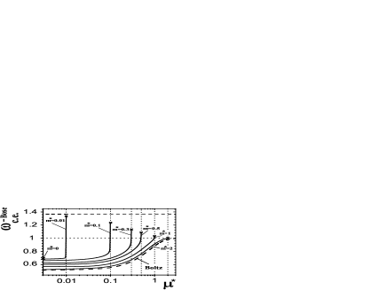
Figure 5: The scaled variances $\omega_{g.c.e.}^{+~{}Bose}$, left, and $\omega_{g.c.e.}^{-~{}Bose}$, right, given by Eq. (37), are shown as functions of $\mu^{*}$. The solid lines present $\omega_{g.c.e.}^{\pm Bose}$ at $m^{*}=0.01,~{}0.1,~{}0.3,~{}0.5,~{}1,~{}2,~{}3$. The vertical dotted lines $\mu^{*}=m^{*}$ demonstrate the restriction $\mu^{*}\leq m^{*}$ in the Bose gas. The dashed horizontal line presents a value of $\zeta(2)/\zeta(3)\simeq 1.368$ which is an upper limit for $\omega_{c.e.}^{\pm~{}Bose}$ reached at $\mu^{*}=m^{*}\rightarrow 0$ (see Eqs.(42,45)). The crosses at $\mu^{*}=m^{*}$ correspond to the points of Bose condensation. The crosses at $\mu^{*}=0$ correspond to $\omega_{c.e.}^{\pm~{}Bose}(\mu^{*}=0,m^{*}\rightarrow 0$ given by Eq. (40). The dashed lines correspond to $\omega_{c.e.}^{+Boltz}$, left and $\omega_{c.e.}^{-Boltz}$, right, given by Eq. (38).

Figure 6: The scaled variances $\omega_{c.e.}^{+Fermi}$ (left) and $\omega_{c.e.}^{-Fermi}$ (right) are presented by the solid lines for $m^{*}=0$ and $m^{*}=2$. The dashed lines correspond to $\omega_{c.e.}^{+Boltz}$ (left) and $\omega_{c.e.}^{-Boltz}$ (right) given by Eq. (38)

At $\mu^{*}=m^{*}\rightarrow\infty$ one finds $\omega_{g.c.e.}^{-~{}Bose}(\mu^{*}=m^{*}\rightarrow\infty)\rightarrow 1$ (see Fig. 4, right). Therefore, it follows:

$$\omega_{c.e.}^{+~{}Bose}(\mu^{*}=m^{*}\rightarrow\infty)~{}\simeq~{}\frac{\rho_{-}^{Bose}(\mu^{*}=m^{*}\rightarrow\infty)}{\rho_{+}^{Bose}(\mu^{*}=m^{*}\rightarrow\infty)}~{}\simeq~{}\frac{1}{\zeta(3/2)}~{}\exp\left(-2\mu^{*}\right)~{}\simeq~{}0.383~{}\exp\left(-2\mu^{*}\right)~{},$$ (43)

so that at $\mu^{*}=m^{*}\rightarrow\infty$ the scaled variance $\omega_{c.e.}^{+~{}Bose}$ goes to zero faster than $\omega_{c.e.}^{+~{}Boltz}\simeq\exp(-2\mu^{*})$. The Fig. 5 (left) demonstrates that $\omega_{c.e.}^{+~{}Bose}(\mu^{*}=m^{*}=1)$ is already smaller than $\omega_{c.e.}^{+~{}Boltz}(\mu^{*}=1)$ (Bose ’suppression’ !).

For $\omega_{c.e.}^{-~{}Bose}(\mu^{*}=m^{*})$ (see Fig. 5, right) one finds from Eq. (37):

$$\omega_{c.e.}^{-~{}Bose}(\mu^{*}=m^{*})~{}=~{}\omega_{g.c.e.}^{-~{}Bose}(\mu^{*}=m^{*})~{},$$ (44)

so that

$$max[\omega_{c.e.}^{-~{}Bose}(\mu^{*},m^{*})]~{}=~{}\omega_{g.c.e.}^{-~{}Bose}(\mu^{*}=0,~{}m^{*}\rightarrow 0)~{}\simeq~{}1.368~{}.$$ (45)

From Eqs. (29,44) it follows,

$$\omega^{-~{}Bose}_{c.e}~{}\simeq~{}1~{}+~{}\gamma~{}2^{-3/2}~{}\exp\left(-~{}2m^{*}\right)~{},$$ (46)

and $\omega_{c.e.}^{-~{}Bose}(\mu^{*}=m^{*}\rightarrow\infty)$ goes to 1 from above (see Fig. 4, right).

Now let us turn to the behavior of $\omega_{c.e.}^{+~{}Fermi}$ and $\omega_{c.e.}^{-~{}Fermi}$ (Fig. 6, left and right, respectively). The variance $\;\sum_{p}v_{p}^{+\,2}\;$ for the Fermi gas increases as $\mu^{*2}$, whereas $\;\sum_{p}v_{p}^{-\,2}\;$ decreases exponentially, $\exp(-\mu^{*})$, for large chemical potentials, $\;\mu^{*}\gg 1\;$. Then it follows from Eq. (37),

$$\omega_{c.e.}^{+~{}Fermi}~{}\simeq~{}\omega_{g.c.e.}^{-~{}Fermi}~{}\times~{}\frac{\rho_{-}^{Fermi}}{\rho_{+}^{Fermi}}~{}\simeq~{}1~{}\times~{}\frac{m^{*2}K_{2}(m^{*})\exp(-\mu^{*})}{\mu^{*3}/3}~{},$$ (47)

for $\mu\rightarrow\infty$. Therefore, $\omega_{c.e.}^{+~{}Fermi}$ goes to zero like $\mu^{*-3}\exp(-\mu^{*})$ as $\mu^{*}\rightarrow\infty$. However, $\omega_{c.e.}^{+~{}Boltz}\simeq\exp(-2\mu^{*})$, and $\omega_{c.e.}^{+~{}Fermi}$ becomes larger than $\omega_{c.e.}^{+~{}Boltz}$ (Fermi ’enhancement’ !) as $\mu^{*}\rightarrow\infty$ (see Fig. 6, left). Finally, using Eqs. (13,33,72) one finds for $\omega_{c.e.}^{-~{}Fermi}$ as $\mu^{*}\rightarrow\infty$:

$$\omega_{c.e.}^{-~{}Fermi}~{} \simeq~{}\omega_{g.c.e.}^{-~{}Fermi}~{}\times~{}\left(1~{}-~{}\frac{\sum_{p}v_{p}^{-~{}2}}{\sum_{p}v_{p}^{+~{}2}}\right)~{}\simeq~{}\left[1~{}-~{}\frac{K_{2}(2m^{*})}{2K_{2}(m^{*})}~{}\exp\left(-~{}\mu^{*}\right)\right]~{}$$

$$\times~{}\left[1~{}-~{}\left(\frac{m^{*}}{\mu^{*}}\right)^{2}K_{2}(m^{*})\exp\left(-\mu^{*}\right)\right]~{}.$$ (48)

Therefore, $\omega_{c.e.}^{-~{}Fermi}$ goes to 1 at $\mu^{*}\rightarrow\infty$ satisfying the inequalities (see Fig. 6, right):

$$\omega_{c.e.}^{-~{}Fermi}~{}<~{}\omega_{g.c.e.}^{-~{}Fermi}~{}<~{}\omega_{c.e.}^{-~{}Boltz}~{}.$$ (49)

VI Summary

The scaled variances for the particle number fluctuations have been systematically studied for the Bose and Fermi ideal relativistic gases. The calculations have been done in the grand canonical and canonical ensembles. The analysis reveals that in the limit of large (positive) chemical potential the quantum effects and effects of the exact charge conservation are absent for negatively charged particles, so that $\omega^{-~{}Bose}\simeq\omega^{-~{}Fermi}\simeq\omega^{-~{}Boltz}\simeq 1$ in both the GCE and CE. However, the strongest quantum effects take place in the limit of large chemical potential for the fluctuations of number of positively charged particles in the GCE (see Fig. 4): $\omega^{+~{}Bose}_{g.c.e.}\rightarrow\infty$ as $\mu^{*}\rightarrow m^{*}$ and $\omega^{+~{}Fermi}_{g.c.e.}\rightarrow 0$ as $\mu^{*}\rightarrow\infty$. On the other hand, just in the limit of large chemical potential we have found the strongest effects of the exact charge conservation. The scaled variances $\omega^{+~{}Bose}_{c.e.}$ and $\omega^{+~{}Fermi}_{c.e.}$ (See Figs. 5 and 6) at large $\mu^{*}$ are very different from those in the GCE. The Bose and Fermi effects in the CE are clearly seen at intermediate $\mu^{*}$, but for $\mu^{*}\gg 1$ the effects of the exact charge conservation dominate: $\omega^{+~{}Bose}_{c.e.}\simeq\omega^{+~{}Boltz}_{c.e.}\rightarrow 0$ at $\mu^{*}=m^{*}\rightarrow\infty$ and $\omega^{+~{}Fermi}_{c.e.}\simeq\omega^{+~{}Boltz}_{c.e.}\rightarrow 0$ at $m\ll\mu\rightarrow\infty$ . The summary of analytical results for some limiting values of the scaled variances for positively and negatively charged particles in the GCE and CE are presented in Table 1.

		$\mu^{*}=0,~{}m^{*}\to 0$	$\mu^{*}=m^{*}\to 0$	$\mu^{*}\ll m^{*}\to\infty$	$\mu^{*}=m^{*}\to\infty$	$m^{*}\ll\mu^{*}\to\infty$
	$\omega^{+~{}Boltz}_{g.c.e}$	1	1	1	1	1
Grand	$\omega^{-~{}Boltz}_{g.c.e}$	1	1	1	1	1
Canonical	$\omega^{+~{}Bose}_{g.c.e}$	1.368	$\infty$	1	$\infty$	—
Ensemble	$\omega^{-~{}Bose}_{g.c.e}$	1.368	1.368	1	1	—
	$\omega^{+~{}Fermi}_{g.c.e}$	0.912	0.912	1	0.791	0
	$\omega^{-~{}Fermi}_{g.c.e}$	0.912	0.912	1	1	1
	$\omega^{+~{}Boltz}_{c.e}$	0.5	0.5	$0.5[1-\tanh(\mu^{*})]$	$0.5[1-\tanh(\mu^{*})]\rightarrow 0$	$0.5[1-\tanh(\mu^{*})]\rightarrow 0$
	$\omega^{-~{}Boltz}_{c.e}$	0.5	0.5	$0.5[1+\tanh(\mu^{*})]$	$0.5[1+\tanh(\mu^{*})]\rightarrow 1$	$0.5[1+\tanh(\mu^{*})]\rightarrow 1$
Canonical	$\omega^{+~{}Bose}_{c.e}$	0.684	1.368	$0.5~{}[1-\tanh(\mu^{*})]$	0	—
Ensemble	$\omega^{-~{}Bose}_{c.e}$	0.684	1.368	$0.5~{}[1+\tanh(\mu^{*})]$	1	—
	$\omega^{+~{}Fermi}_{c.e}$	0.456	0.456	$0.5~{}[1-\tanh(\mu^{*})]$	0	0
	$\omega^{-~{}Fermi}_{c.e}$	0.456	0.456	$0.5~{}[1+\tanh(\mu^{*})]$	1	1

Table 1: The scaled variances $\omega^{+}$ and $\omega^{-}$ for different statistics in the GCE and CE. The values of $\mu^{*}>m^{*}$ are forbidden in the Bose gas.

Appendix A

An integral representation of the modified Hankel function $K_{2}$ has the form AS :

$$K_{2}\left(n\,m^{*}\right)~{}=~{}n~{}m^{*\,-2}~{}\int_{0}^{\infty}x^{2}dx~{}\exp\left(-n\,\sqrt{m^{*2}+x^{2}}\right)~{}.$$ (50)

The asymptotic behavior of the $K_{2}$ function at large and small arguments is the following:

$$K_{2}(y)\; \simeq\;\sqrt{\frac{\pi}{2y}}\,\exp(-y)\;,~{}~{}~{}~{}y~{}\gg~{}~{}1~{};$$ (51)

$$K_{2}(y)\; \simeq\;2~{}y^{-2}\;,~{}~{}~{}~{}~{}~{}y~{}\ll~{}~{}1~{}.$$ (52)

Using for $z>0$ the expansions ($\gamma=+1,-1,0$),

$$\frac{1}{\exp(z)~{}-~{}\gamma}\;=\;\sum_{n=1}^{\infty}\gamma^{n-1}\exp(-n\,z)\;,~{}~{}~{}~{}~{}\frac{1}{\left(\exp(z)~{}-~{}\gamma\right)^{2}}\;=\;\sum_{n=1}^{\infty}\gamma^{n-1}\,n\;\exp[-(n+1)\,z]\;,$$ (53)

one finds at $\mu^{*}\leq m^{*}$:

$$\int_{0}^{\infty}\frac{x^{2}dx}{\exp\left[\left(\sqrt{m^{*2}+x^{2}}\mp\mu^{*}\right)\right]~{}-~{}\gamma} \;=\;m^{*2}~{}\sum_{n=1}^{\infty}\frac{\gamma^{n-1}}{n}\,K_{2}\left(n\,m^{*}\right)\exp\left(\pm n\mu^{*}\right)\;,$$ (54)

$$\int_{0}^{\infty}\frac{x^{2}dx}{\left[\;\exp\left[\left(\sqrt{m^{*2}+x^{2}}\mp\mu\right)\right]~{}-~{}\gamma\;\right]^{2}} \;=\;m^{*2}~{}\sum_{n=1}^{\infty}\frac{\gamma^{n-1}~{}n}{n+1}K_{2}\left[(n+1)\,m^{*}\right]\exp\left[\pm(n+1)\mu^{*}\right]\;.$$ (55)

The polylogarithm function (or Jonquière’s function) is defined as PBM

$$Li_{k}(z)~{}=~{}\sum_{n=1}^{\infty}~{}\frac{z^{n}}{n^{k}}~{}.$$ (56)

For $\;z=1\;$ it equals the Riemann zeta function,

$$\zeta(k)~{}=~{}\sum_{n=1}^{\infty}~{}\frac{1}{n^{k}}~{}.$$ (57)

Some special values of the zeta function used in the paper are:

$$\zeta\left(\frac{3}{2}\right)~{}\simeq~{}2.612~{},~{}~{}~{}~{}\zeta\left(2\right)~{}=~{}\frac{\pi^{2}}{6}~{}\simeq~{}1.645,~{}~{}~{}~{}\zeta\left(3\right)~{}\simeq~{}1.202,~{}~{}~{}~{}\zeta\left(4\right)\;=\;\frac{\pi^{4}}{90}~{}\simeq~{}1.082~{}.$$ (58)

Appendix B

To obtain the asymptotic expansion of $\rho_{+}^{Fermi}$ at $\mu^{*}\gg m^{*}$ one calculates making the variable substitutions and integrating by parts:

$$\int_{0}^{\infty}\frac{x^{2}dx}{\exp\left(\sqrt{m^{*2}+x^{2}}-\mu^{*}\right)+1}=\int_{m^{*}}^{\infty}\frac{\sqrt{\epsilon^{2}-m^{*2}}~{}\epsilon~{}d\epsilon}{\exp\left(\epsilon-\mu^{*}\right)+1}=\frac{1}{3}\int_{m^{*}-\mu^{*}}^{\infty}dy~{}[(y+\mu^{*})^{2}-m^{*2}]^{3/2}~{}\frac{\exp(y)}{[\exp(y)+1]^{2}}$$

$$~{}\equiv~{}\frac{1}{3}\int_{m^{*}-\mu^{*}}^{\infty}~{}dy~{}f(y)~{}\frac{\exp(y)}{[\exp(y)+1]^{2}}~{}.$$ (59)

The function $\exp(y)[\exp(y)+1]^{-2}$ has a maximum at $y=0$ and decreases exponentially at $y\rightarrow\pm\infty$. Expanding the function $f(y)$ in a Taylor series at $y=0$ and extending the lower limit of the $y$-integral in Eq. (59) to $-\infty$ (this adds only exponentially small term proportional to $\exp(-\mu^{*})$) one finds an asymptotic expansion at $\mu^{*}\gg m^{*}$:

$$\frac{1}{3}\int_{m^{*}-\mu^{*}}^{\infty}~{}dy~{}f(y)~{}\frac{\exp(y)}{[\exp(y)+1]^{2}}~{}\simeq~{}\frac{1}{3}\int_{-\infty}^{\infty}~{}dy~{}\left[f(0)~{}+~{}f^{\prime}(0)~{}y~{}+~{}\frac{1}{2}~{}f^{\prime\prime}(0)~{}y^{2}~{}+~{}\ldots~{}\right]~{}\frac{\exp(y)}{[\exp(y)+1]^{2}}.$$ (60)

It follows for $f(0)$ and its derivatives

$$f(0)~{}=~{}(\mu^{*~{}2}~{}-~{}m^{*~{}2})^{3/2}~{},~{}~{}~{}~{}f^{\prime}(0)~{}=~{}3\mu^{*}~{}(\mu^{*~{}2}~{}-~{}m^{*~{}2})^{1/2}~{},~{}~{}~{}~{}f^{\prime\prime}(0)~{}=~{}3~{}\frac{2\mu^{*~{}2}~{}-~{}m^{*~{}2}}{(\mu^{*~{}2}~{}-~{}m^{*~{}2})^{1/2}}\;,$$ (61)

so that $f^{(n)}(0)\propto(\mu^{*})^{3-n}$ as $\mu^{*}\rightarrow\infty$. The remaining $y$-integrals are equal to PBM :

$$I_{0}~{} =~{}\int_{-\infty}^{\infty}dy~{}\frac{\exp(y)}{[\exp(y)~{}+~{}1]^{2}}~{}=~{}1~{},$$ (62)

$$I_{n}\; =\;\int_{-\infty}^{\infty}~{}dy~{}y^{n}~{}\frac{\exp(y)}{[\exp(y)~{}+~{}1]^{2}}~{}=~{}2~{}n!~{}\sum_{k=1}^{\infty}\frac{(-1)^{k+1}}{k^{n}}~{}=~{}2~{}n!~{}(1~{}-~{}2^{-n+1})~{}\zeta(n)~{},$$ (63)

for even $n=2l$, and $I_{n}=0$ for odd $n=2l-1$, ($l=1,2,3,\ldots$). One finally obtains:

$$\int_{0}^{\infty}\frac{x^{2}dx}{\exp\left(\sqrt{m^{*2}+x^{2}}-\mu^{*}\right)+1}~{}\simeq~{}\frac{1}{3}~{}\left[f(0)~{}I_{0}~{}+~{}\frac{1}{2}\;f^{\prime\prime}(0)~{}I_{2}~{}+~{}\ldots~{}\right]$$

$$=~{}\frac{1}{3}~{}(\mu^{*~{}2}~{}-~{}m^{*~{}2})^{3/2}~{}...+~{}\frac{2\mu^{*~{}2}~{}-~{}m^{*~{}2}}{(\mu^{*~{}2}~{}-~{}m^{*~{}2})^{1/2}}~{}\zeta(2)~{}+~{}\ldots~{}\simeq\;\frac{1}{3}\;\mu^{*\,3}+\left(\frac{\pi^{2}}{3}-\frac{m^{*\,2}}{2}\right)\mu^{*}+\ldots~{}.$$ (64)

To find $\omega^{+~{}Fermi}$ at $\mu^{*}\gg m^{*}$ one needs to calculate integral (26) for $\alpha=-\gamma=1$ (note that $\omega^{-Fermi}\simeq\omega^{-Boltz}=1$ in this limit). Similar to Eqs. (59,60) one finds:

$$\int_{0}^{\infty}\frac{x^{2}dx}{\left[\;\exp\left(\sqrt{x^{2}+m^{*\,2}}~{}+\mu^{*}\right)~{}+~{}1\;\right]^{2}}~{}$$

$$\simeq~{}\frac{2}{3}\int_{-\infty}^{\infty}~{}dy~{}\left[f(y_{0})~{}+~{}f^{\prime}(y_{0})~{}(y~{}-y_{0})~{}+~{}\frac{1}{2}~{}f^{\prime\prime}(y_{0})~{}(y~{}-~{}y_{0})^{2}~{}+~{}\ldots~{}\right]~{}\frac{\exp(y)}{[\exp(y)+1]^{3}}~{},$$ (65)

where $y_{0}=-\ln 2$ is the point of maximum for the function $\exp(y)[\exp(y)+1]^{-3}$. The $y$-integrals in Eq. (65) are equal to GR :

$$A_{0}~{} =~{}\int_{-\infty}^{\infty}dy~{}\frac{\exp(y)}{[\exp(y)~{}+~{}1]^{3}}~{}=~{}\frac{1}{2}~{},$$ (66)

$$A_{1}\; =\;\int_{-\infty}^{\infty}~{}dy~{}\frac{y~{}\exp(y)}{[\exp(y)~{}+~{}1]^{3}}~{}=~{}-\frac{1}{2}~{},$$ (67)

$$A_{2}\; =\;\int_{-\infty}^{\infty}~{}dy~{}\frac{y^{2}~{}\exp(y)}{[\exp(y)~{}+~{}1]^{3}}~{}=~{}\frac{\pi^{2}}{6}~{}.$$ (68)

One finds:

$$\int_{0}^{\infty}\frac{x^{2}dx}{\left[\exp\left(\sqrt{m^{*2}+x^{2}}-\mu^{*}\right)+1\right]^{2}}$$

$$\simeq~{}\frac{2}{3}~{}\left[f(y_{0})~{}A_{0}~{}+~{}f^{\prime}(y_{0})~{}(A_{1}~{}-~{}y_{0}~{}A_{0})~{}+~{}\frac{1}{2}~{}f^{\prime\prime}(y_{0})~{}(A_{2}~{}-~{}2y_{0}~{}A_{1}~{}+~{}y_{0}^{2}~{}A_{0})~{}+~{}\ldots~{}\right]$$

$$\simeq\;\frac{1}{3}\;\mu^{*\,3}-\mu^{*\,2}+\left(\frac{\pi^{2}}{3}-\frac{m^{*\,2}}{2}\right)\mu^{*}+\ldots$$ (69)

Thus for Fermi particles at $\mu^{*}\rightarrow\infty$ the following expansions are obtained:

$$\sum_{p}\langle n_{p}^{+}\rangle_{g.ce.} \;\simeq\;\frac{g\,V\,T^{3}}{2\pi^{2}}\left[\frac{1}{3}\;\mu^{*\,3}+\left(\frac{\pi^{2}}{3}-\frac{m^{*\,2}}{2}\right)\mu^{*}\right]\;,$$ (70)

$$\sum_{p}\langle n_{p}^{+\,2}\rangle_{g.c.e.} \;\simeq\;\frac{g\,V\,T^{3}}{2\pi^{2}}\left[\frac{1}{3}\;\mu^{*\,3}-\mu^{*\,2}+\left(\frac{\pi^{2}}{3}-\frac{m^{*\,2}}{2}\right)\mu^{*}\right]\;=\;\sum_{p}\langle n_{p}^{+}\rangle_{g.c.e.}-\frac{g\,V\,T^{3}}{2\pi^{2}}\;\mu^{*\,2}\;,$$ (71)

$$\sum_{p}v_{p}^{+\,2} \;\equiv\;\sum_{p}\langle n_{p}^{+}\rangle_{g.c.e.}\;-\;\sum_{p}\langle n_{p}^{+2}\rangle_{g.c.e.}\;\simeq\;\frac{g\,V\,T^{3}}{2\pi^{2}}\;\mu^{*\,2}~{}.$$ (72)

References

(1)
J. Cleymans and H. Satz, Z. Phys. C 57, 135 (1993); J.
Sollfrank, M. Gaździcki, U. Heinz, and J. Rafelski, ibid.61, 659 (1994); G.D. Yen, M.I. Gorenstein, W. Greiner, and
S.N. Yang, Phys. Rev. C 56, 2210 (1997); F. Becattini, M.
Gaździcki, and J. Solfrank, Eur. Phys. J. C 5, 143
(1998); G.D. Yen and M.I. Gorenstein, Phys. Rev. C 59,
2788 (1999); P. Braun-Munzinger, I. Heppe and J. Stachel, Phys.
Lett. B 465, 15 (1999); P. Braun-Munzinger, D. Magestro, K.
Redlich, and J. Stachel, ibid.518, 41(2001);
F. Becattini, M. Gaździcki, A. Keränen, J. Mannienen, and
R. Stock, Phys. Rev. C 69, 024905 (2004).
(2)
P. Braun-Munzinger, K. Redlich, J. Stachel, nucl-th/0304013,
Review for Quark Gluon Plasma 3, eds. R.C. Hwa and X.-N. Wang,
World Scientific,Singapore.
(3)
R. Hagedorn, CERN Report 71-12 (1971); E.V. Shuryak, Phys. Lett. B
42, 357 (1972).
(4)
K. Redlich and L. Turko, Z. Phys. C 5, 541 (1980); J.
Rafelski and M. Danos, Phys. Lett. B 97, 279 (1980) ; L.
Turko, ibid B 104, 153 (1981); R. Hagedorn and K.
Redlich, Z. Phys. C 27, 541 (1985); L. Turko and J.
Rafelsky, Eur. Phys. J. C 18, 587 (2001).
(5)
F. Becattini, Z. Phys. C 69, 485 (1996); F. Becattini, U.
Heinz, ibid.76, 269 (1997); F. Becattini, G.
Passaleva, Eur. Phys. J. C 23, 551 (2002).
(6)
J. Cleymans, K Redlich, E. Suhonen, Z. Phys. C 51, 137
(1991); J. Cleymans, K Redlich, and E Suhonen, Z. Phys. C 58, 347 (1993); J. Cleymans, M. Marais, E. Suhonen, Phys. Rev. C
56, 2747 (1997); J. Cleymans, H. Oeschler, K. Redlich, Phys.
Rev. C 59, 1663 (1999); Phys. Lett. B 485, 27 (2000);
J.S. Hamieh, K. Redlich, and A. Tounsi, Phys. Lett. B 486,
61 (2000); J. Phys. G 27, 413 (2001); P. Braun-Munzinger,
J. Cleymans, H. Oeschler, and K. Redlich, Nucl. Phys. A 697,
902 (2002); A. Tounsi, A. Mischke, and K. Redlich, Nucl. Phys. A
715, 565 (2003).
(7)
M.I. Gorenstein, M. Gaździcki, and W. Greiner, Phys. Lett. B
483, 60 (2000).
(8) M.I. Gorenstein, A.P. Kostyuk, H. Stöcker,
and W. Greiner, Phys. Lett. B 509, 277 (2001).
(9)
K. Werener and J. Aichelin, Phys. Rev. C 52, 1584 (1995);
F. Liu, K. Werner and J. Aichelin, ibid68, 024905
(2003); F. Liu, K. Werner, J. Aichelin, M. Bleicher, and
H. Stöcker, J. Phys. G 30, S589 (2004);
F. Becattini and L. Ferroni, Eur. Phys. J. C 35, 243(2004);
Eur.Phys.J. C38 (2004) 225-246.
(10)
H. Heiselberg, Phys. Rep. 351, 161 (2001);
S. Jeon and V. Koch, hep-ph/0304012, Review for Quark-Gluon Plasma
3, eds. R.C. Hwa and X.-N. Wang, World Scientific, Singapore.
(11) M.A. Stephanov, K. Rajagopal, and E.V. Shuryak,
Phys. Rev. Lett. 81, 4816 (1998); M.A. Stephanov, Acta
Phys. Polon. B 35, 2939 (2004).
(12)
M.A. Stephanov, K. Rajagopal, and E.V. Shuryak, Phys. Rev. D 60, 114028 (1999).
(13) M. Gaździcki, M.I.
Gorenstein, and St. Mrówczyński, Phys. Lett. B 585,
115 (2004);
M.I. Gorenstein, M. Gaździcki, and O.S. Zozulya, ibid.585, 237 (2004);
M. Gaździcki, nucl-ex/0507017.
(14) V.V. Begun, M. Gaździcki, M.I. Gorenstein, and O.S. Zozulya,
Phys. Rev. C 70, 034901 (2004).
(15) V.V. Begun, M.I. Gorenstein, and O.S. Zozulya,
nucl-th/0411003
(16) A. Keränen, F. Becattini, V.V. Begun,
M.I. Gorenstein, and O.S. Zozulya, J. Phys. G 31, S1095
(2005).
(17)
F. Becattini, A. Keranen, L. Ferroni, T. Gabbriellini,
nucl-th/0507039.
(18) V.V. Begun, M.I. Gorenstein, A.P. Kostyuk,
and O.S. Zozulya, Phys. Rev. C 71, 054904 (2005).
(19) V.V. Begun, M.I. Gorenstein, A.P. Kostyuk,
and O.S. Zozulya, nucl-th/0505069
(20)
J. Cleymans, K. Redlich, L. Turko, Phys. Rev. C 71, 047902
(2005); J. Cleymans, K. Redlich, L. Turko, hep-th/0503133.
(21)
L.D. Landau and E.M. Lifschitz, Statistical Physics
(Fizmatlit, Moscow, 2001); W. Greiner, L. Neise, and
H. Stöcker, Thermodynamic and Statistical Mechanic
(Verlag harri Deursch, Frankfurt, 1987).
(22)
L. Salasnich, Nuovo Cim. B 117, 637 (2002).
(23)
M. Abramowitz and I.E. Stegun,
Handbook of Mathematical Functions (Dover, New York, 1964).
(24)
A.P. Prudnikov, Yu.A. Brychkov, and O.I. Marichev, Integrals
and Series, (Moscow, Nauka, 1986).
(25)
I.S. Gradstein and I.M. Ryzhik, Tables of Integrals, Series,
and Products, (Moscow, Nauka, 1971).