The Two–Body Random Ensemble in Nuclei

Abstract

Combining analytical and numerical methods, we investigate properties of the two–body random ensemble (TBRE). We compare the TBRE with the Gaussian orthogonal ensemble of random matrices. Using the geometric properties of the nuclear shell model, we discuss the information content of nuclear spectra, and gain insight in the difficulties encountered when fitting the effective interaction. We exhibit the existence of correlations between spectral widths pertaining to different quantum numbers. Using these results, we deduce the preponderance of spin–zero ground states in the TBRE. We demonstrate the existence of correlations between spectra with different quantum numbers and/or in different nuclei.

I Introduction

The spectral fluctuation properties of complex nuclear spectra often agree with predictions of random–matrix theory, more precisely: With those of the Gaussian orthogonal ensemble of random matrices (GOE). This is true for the resonances observed at neutron threshold and at the Coulomb barrier for protons HPB but applies in a number of cases likewise to levels at lower excitation energies, see Ref. AHSW and references therein.

The GOE is an ensemble of matrices where every state in Hilbert space interacts with every other state (if both carry the same conserved quantum numbers). Indeed, the probability density ${\cal P}(H_{\rm GOE})$ of the real and symmetric Hamiltonian matrices $H_{\rm GOE}$ of the GOE has the form

$${\cal P}(H_{\rm GOE})={\cal N}\exp\big{\{}-\frac{N}{\lambda^{2}}{\rm Trace}[H_{\rm GOE}^{2}]\big{\}}$$ (1)

where $N$ denotes the dimension of the matrices and $\lambda$ a parameter which determines the average level density while ${\cal N}$ is a normalization factor. Eq. (1) shows that the matrix elements connecting any pair of states are uncorrelated Gaussian–distributed random variables.

This basic tenet of the GOE is not in keeping with the shell model, the fundamental dynamical model of nuclear physics MJ . Indeed, that model is basically a single–particle model with a residual interaction. The interaction is dominated by two–body forces. In a representation where the many–body states are Slater determinants of single–particle states, a two–body interaction will have non–zero matrix elements only between those Slater determinants which differ by at most two units in the occupation numbers of the single–particle states. Out of the total number of such determinants, this is a small fraction. Put differently: In an arbitrary basis for the many–body states, the number of independent matrix elements of the two–body interaction is very much smaller than that of the GOE. This fact is changed only quantitatively but not qualitatively when we allow for a three–body residual interaction.

Already in the 1970’s, this fact has led to the question: Are the predictions of the GOE for spectral fluctuation properties in keeping with the results of shell–model calculations with a residual two–body interaction? The answer, based on numerical calculations, has been affirmative FW ; BF , and numerous more recent calculations have confirmed it (see the review ZE and references therein). The calculations were based upon a random–matrix ensemble (the two–body random ensemble (TBRE)) which differs from the GOE and accounts for the specific properties of the nuclear shell model: The existence of a residual two–body interaction which conserves total spin, parity, and isospin.

In spite of the agreement between GOE predictions and numerical results for the TBRE, open questions remain. In fact, analytical studies of the TBRE are virtually non–existent. Treating the TBRE analytically poses a severe challenge. We use a combination of numerical and analytical techniques to display some of its properties. We focus on the underlying geometric structure of the TBRE and its implications for correlations between spectra of different quantum numbers (like nucleon number and/or spin). The results we are obtain are interesting also from a practical point of view, as we gain insight into the inner workings of the shell model and are able to separate geometric and dynamical properties. Together with the work reported in Refs. PW ; PW1 , the present paper may be seen as a step towards filling the gap in understanding the TBRE.

In treating the TBRE, we neglect the influence of possible three–body forces. It will become clear below that this omission affects our results in a quantitative but not in a qualitative fashion. Spectral fluctuation properties of the GOE type emerge only when there are at least three nucleons in a major shell. This is why we confine ourselves to this case.

This paper is organized as follows. The two–body random ensemble is defined and compared with the GOE in Section II. Some of basic properties of the TBRE are displayed in Section III. This main section contains results about the information content of nuclear spectra, the preponderance of spin-0 ground states, and correlations between spectra with different quantum numbers. Section IV contains a brief summary. Technical details are relegated to several Appendices.

II Definition of the TBRE

The two–body random ensemble (TBRE) is defined within the framework of the spherical nuclear shell model MJ . In that model, nucleons move independently in a central potential with a strong spin–orbit force. We consider one of the major shells of that model. Our numerical examples are calculated for the $sd$–shell, with single–particle states labelled $s_{1/2},d_{3/2}$, and $d_{5/2}$ and single–particle energies $\varepsilon_{1/2},\varepsilon_{3/2}$, and $\varepsilon_{5/2}$. Our general considerations apply likewise, however, to other major shells in heavier nuclei. There, however, the number of many–particle states becomes forbiddingly large for numerical work. We sometimes also consider a single $j$–shell with half–integer single–particle total spin $j$. Although not realistic for nuclei, this case is sufficiently simple to yield useful insights.

Putting several nucleons into a major shell, we construct a basis of orthonormal antisymmetrized many–body states of fixed total spin $J$, parity $P$, and isospin $T$. These states are labelled $|{\bf J}\mu\rangle$, with ${\bf J}$ standing for the three quantum numbers $J,P,T$ and with $\mu=1,\ldots,d({\bf J})$ a running index with range given by the dimension $d({\bf J})$ of Hilbert space ${\cal H}({\bf J})$. We focus attention on a fixed but arbitrary $z$–projection $M$ of total spin $J$ so that $d({\bf J})$ is the actual number of states not counting their degeneracy regarding $M$. In the middle of the $sd$–shell and for low values of $J$, $d({\bf J})$ is typically of order $10^{3}$ and much larger for heavier nuclei (other major shells). The actual construction used for the basis of states $|{\bf J}\mu\rangle$ is immaterial for what follows: The bases resulting from different modes of construction are connected by a unitary transformation. In the $sd$–shell, all single–particle states have positive parity, and it is not neccessary to carry the quantum number $P$. Likewise, we often consider only $sd$–shell states with isospin $T=0$. In that case, it suffices to label the many–body states by the total spin $J$ only.

The number of nucleons in the major shell is denoted by $m$. Sometimes, we will consider simultaneously several nuclei with different values of $m$. In this case, we will denote, f.i., the dimension of Hilbert space by $d({\bf J},m)$, and similarly for other quantities.

The many–body states $|{\bf J}\mu\rangle$ are eigenstates of the single–particle shell–model Hamiltonian with a very high degree of degeneracy. The degeneracy is lifted when we take account of the residual interaction of the shell model. We assume that this interaction mixes states only within the same major shell. That assumption is rather unrealistic because intruder states from higher shells occur even at low excitation energies, and mixing with higher shells is bound to play a major role at the upper end of the spectrum. The approximation is perfectly adequate, however, for the purposes of this paper. For the same reason we confine ourselves to a two–body residual interaction (although there is evidence that three–body forces do play a role in realistic attempts to model the spectrum), and we omit the Coulomb interaction between protons. Finally, to focus attention on the role of the residual interaction, we assume that the single–particle energies within a major shell are all degenerate. For the $sd$–shell, this means that we put $\varepsilon_{1/2}=\varepsilon_{3/2}=\varepsilon_{5/2}=0$. Then, the full Hamiltonian $H$ of the shell model is determined entirely by the residual interaction. In the sequel we consider the matrix elements $H_{\mu\nu}({\bf J})$ of that Hamiltonian taken with respect to the basis of states $|{\bf J}\mu\rangle$.

Within a major shell, the residual two–body interaction $V_{2}$ possesses a finite number of two–body matrix elements. These have the following form. Let ${\bf j}_{i}$, $i=1,2,3,4$ denote 4 (equal or different) values of total single–particle spin, parity, and isospin $1/2$. Coupling ${\bf j}_{1}$ and ${\bf j}_{2}$ (${\bf j}_{3}$ and ${\bf j}_{4}$) to total two–body spin $s_{1}$ ($s_{2}$, repectively) and isospin $t_{1}$ ($t_{2}$, respectively), denoting the parity of the resulting wave functions by $\pi_{1}$ ($\pi_{2}$, respectively), and introducing the notation ${\bf s}$ for the quantum numbers $s,\pi,t$, the reduced two–body matrix elements of $V_{2}$ within a major shell have the form $\langle{\bf j}_{3}{\bf j}_{4}{\bf s}||V_{2}||{\bf j}_{1}{\bf j}_{2}{\bf s}\rangle$ where we have put ${\bf s}_{1}={\bf s}_{2}={\bf s}$ since $V_{2}$ conserves spin, parity, and isospin. The number $a$ of such two–body matrix elements within a major shell is limited. For the $sd$–shell, we have $a=63$, while for a single $j$–shell and identical nucleons, $a=j+1/2$. For brevity, we denote these matrix elements by $v_{\alpha}$ with $\alpha=1,\ldots,a$. We use the label $\alpha$ also for the specific two–body operator the two–body matrix element of which is $v_{\alpha}$, see Appendix 1. Within a major shell, $V_{2}$ is characterized completely by the $a$ matrix elements $v_{\alpha}$, no matter how complicated the actual form of $V_{2}$.

The Hamiltonian of the shell model is linear in the matrix elements $v_{\alpha}$ and has the form

$$H_{\mu\nu}({\bf J})=\sum_{\alpha}v_{\alpha}C_{\mu\nu}({\bf J},\alpha)\ .$$ (2)

The matrices $C_{\mu\nu}({\bf J},\alpha)$ transport the two–body interaction into the Hilbert space ${\cal H}({\bf J})$ and depend upon the quantum numbers ${\bf J}$, upon the particular states $\mu$ and $\nu$, and upon the particular two–body operator $\alpha$ considered. The values of the $C_{\mu\nu}({\bf J},\alpha)$’s are completely specified by the underlying shell model, i.e., the single–particle states that occur within the given major shell, the coupling scheme used to construct the many–body states $|{\bf J}\mu\rangle$, and by the exclusion principle. The matrices $C_{\mu\nu}({\bf J},\alpha)$ do not depend upon the choice of the two–body interaction. That choice is specified by the values of the matrix elements $v_{\alpha}$. Eq. (2) yields a decomposition of $H$ into parts which are determined entirely by the symmetries of the shell model (the matrices $C_{\mu\nu}({\bf J},\alpha)$), and parts which carry the information on the specific details of the two–body interaction (the matrix elements $v_{\alpha}$).

We aim at generic statements about spectral properties of $H$ which apply to (almost) all two–body residual interactions. To this end we employ the TBRE: The matrix elements $v_{\alpha}$ are assumed to be uncorrelated Gaussian–distributed random variables with mean values zero and a common second moment $v^{2}$. Without loss of generality we put $v^{2}=1$ (we recall that all single–particle energies are equal so that the scale of the spectrum is determined by $v^{2}$). Mean values of observables are worked out by integrating over the random variables $v_{\alpha}$, the measure being given by the product of the differentials of the $v_{\alpha}$’s and a Gaussian factor $\exp(-\sum_{\alpha}v^{2}(\alpha)/2)$. Having calculated the mean value and the square root of the variance of an observable, we are sure that (within the error given by the latter) the mean value applies to all members of the ensemble, i.e., to all two–body interactions, with the exception of a set of measure zero. With the $v_{\alpha}$’s Gaussian random variables, the Hamiltonian $H_{\mu\nu}({\bf J})$ represents an ensemble of Gaussian–distributed random matrices, the TBRE.

As mentioned in the Introduction, numerical studies have shown that the spectral fluctuation properties of the TBRE generically coincide with those of the GOE. That result is tantamount to saying that $H$ mixes the basis states $|{\bf J}\mu\rangle$ completely, irrespective of the specific choice of the $v_{\alpha}$’s, and, thus, reflects a property of the matrices $C_{\mu\nu}({\bf J},\alpha)$: Almost every linear combination of these matrices must be a sufficiently dense matrix in Hilbert space ${\cal H}({\bf J})$, with matrix elements which are sufficiently complex, to achieve such mixing. This statement is rather remarkable because the matrices $C_{\mu\nu}({\bf J},\alpha)$ are defined entirely in terms of an independent–particle model (which is integrable). In principle, the $C_{\mu\nu}({\bf J},\alpha)$’s can be worked out using group–theoretical methods! Intuitively, that mixing property of the $C_{\mu\nu}({\bf J},\alpha)$’s can be understood by observing that each matrix element of $C_{\mu\nu}({\bf J},\alpha)$ contains sums of products of Clebsch–Gordan and Racah coefficients and coefficients of fractional parentage. For more than three particles in a major shell, the combination of these coefficients is highly complex, even though each one of them is well–defined and simple. A more detailed discussion of the properties of the matrices $C_{\mu\nu}({\bf J},\alpha)$ was given in Ref. PW . Some further properties are displayed in Appendix 2. We show, in particular, that the $C_{\mu\nu}({\bf J},\alpha)$’s do not commute.

Before exploring some properties of the TBRE in the next Section, we compare the TBRE with the GOE. To this end, we recall some properties of the GOE, see Eq. (1). The number of independent matrix elements of the GOE is $N(N+1)/2$. That is also the number of uncorrelated random variables which is, thus, very much larger than the dimension $N$ of the matrices if $N\gg 1$. Except for the symmetry of the GOE Hamiltonian $H_{\rm GOE}$ about the main diagonal, each matrix element carries an independent random variable. The situation is very different for the TBRE. Here, the number $a$ of independent random variables is typically much smaller than the dimension $d({\bf J})$ of Hilbert space. The complete mixing of the basis states and the ensuing validity of Wigner–Dyson statistics for the spectrum cannot be achieved by such a small number of random variables alone. In an essential way it is also due to the matrices $C_{\mu\nu}({\bf J},\alpha)$. These matrices form a fixed “scaffolding” for the TBRE. Although determined group–theoretically, these matrices are sufficiently dense and complex to guarantee complete mixing of Hilbert space for almost all choices of the random variables $v_{\alpha}$.

The GOE is invariant under orthogonal transformations. Moreover, it is universal (i.e., the local spectral fluctuation properties do not depend upon the assumption that the ensemble has a Gaussian distribution) and ergodic (i.e., in the limit $N\to\infty$ and for almost all members of the ensemble, the running average of an observable taken over the spectrum of a single member of the ensemble is equal to the ensemble average of that observable taken at fixed energy). These properties make the GOE to a formally attractive, mathematically accessible and universal model for stochastic spectral fluctuations. Does the TBRE possess any of these properties? The TBRE is manifestly not invariant under orthogonal transformations since the matrices $C({\bf J},\alpha)$ are fixed by the underlying shell model. It is not clear whether the TBRE is universal. One might think, for instance, of modifying the TBRE in such a way that it incorporates known features of the two–body interaction. One such feature is the pairing force. Doing so would impose certain fixed relations among the random variables $v_{\alpha}$. One could then assume that the remaining unconstrained random variables have a Gaussian distribution. It is not known whether such a constrained TBRE would still generically possess spectral fluctuations of the GOE type. Finally, the ensemble is not ergodic. Indeed, ergodicity presupposes that the limit of infinite matrix dimension can be taken. But the matrices $C({\bf J},\alpha)$ of the TBRE have fixed dimension, and the question of ergodicity cannot even be formulated meaningfully in this context. The only exception is the model of a single $j$–shell for which the limit $j\to\infty$ is meaningful (it shares this property with French’s embedded ensembles). It is not known whether in that limit, the TBRE for a single $j$–shell is ergodic.

From all these points of view, the GOE is clearly the more attractive model for stochastic spectral fluctuations. Why then bother with the TBRE which is mathematically so much more complicated and unrewarding? The TBRE offers the singular advantage of combining stochastic modelling with a realistic description of nuclear spectral properties. This leads to specific insights which go beyond the realm of canonical random–matrix theory. Some of these are explored in the sequel.

III Properties of the TBRE

For a full theoretical treatment of the TBRE, we would need a thorough analytical understanding of the properties of the matrices $C_{\mu\nu}({\bf J},\alpha)$. Unfortunately, we are still far from this goal. We confine ourselves in this Section to a number of results which illuminate some properties of the TBRE.

III.1 Information Content of Nuclear Spectra

Almost by definition, a GOE spectrum carries no information beyond the symmetry of the Hamiltonian about the main diagonal. Indeed, the $N(N+1)/2$ matrix elements of the Hamiltonian are drawn at random from a Gaussian probability distribution. Conversely, how many pieces of information are needed to reconstruct the GOE Hamiltonian from the spectrum? Knowledge of all the $N$ eigenvalues does not suffice. Knowledge of one eigenfunction adds $N-1$ additional pieces of information (all expansion coefficients with respect to a fixed basis except for the constraint due to normalization); knowledge of a second eigenfunction adds another $N-2$ such pieces (all expansion coefficients constrained by normalization and orthogonality to the first eigenfunction). Continuing that way, we see that the knowledge of all eigenvalues and of all eigenfunctions is needed to reconstruct the original GOE Hamiltonian. Since a GOE Hamiltonian does not carry any information, it is useless to investigate a GOE spectrum spectroscopically.

Can we conclude from this result that whenever a spectrum displays Wigner–Dyson statistics, it is useless to apply spectroscopy? In particular, would such a statement hold for nuclei? If not, which is the information content of a nuclear spectrum? These are the questions behind the title of the present Subsection.

The answer to the first two questions is obviously a resounding NO. A Hamiltonian of the TBRE is specified by the choice of the $a$ random variables $v_{\alpha}$. We recall that $a$ is typically much smaller than $d({\bf J})$, the dimension of Hilbert space of the many–body states with quantum numbers ${\bf J}$. Therefore, the knowledge of $a\ll d({\bf J})$ independent pieces of information from a spectrum of states with quantum numbers ${\bf J}$ alone will suffice to determine not only $H({\bf J})$ but also the Hamiltonian matrices $H({\bf J^{\prime}})$ of all other quantum numbers ${\bf J^{\prime}}\neq{\bf J}$! (This statement carries a small proviso: All the eigenvalues $s^{2}_{\alpha}({\bf J})$ defined in Eq. (4) below must differ from zero. Otherwise, additional information from spectra with ${\bf J}^{\prime}\neq{\bf J}$ is needed). Given more than $a$ pieces of data, the system of equations for the $a$ matrix elements $v_{\alpha}$ is obviously overdetermined, and nuclear spectroscopy is eminently meaningful even though the spectra may display Wigner–Dyson statistics. This conclusion is not confined to low excitation energies but applies, in principle, also to the domain of slow neutron resonances. The reason is that the mixing of basis states which leads to Wigner–Dyson statistics, is mainly due to the scaffolding matrices $C_{\mu\nu}({\bf J},\alpha)$ which are fixed by the shell model.

Can we identify the $a$ independent pieces of information which are best suited to determine the variables $v_{\alpha}$? More importantly, do such $a$ independent pieces of information always exist? To answer these questions, it is useful to rewrite the TBRE in another form. We use the fact that such questions are most easily addressed in the framework of linear independence and orthogonality. The matrices $C({\bf J},\alpha)$ span a linear space ${\cal S}$. In ${\cal S}$, the Hamiltonian (2) can be viewed as a vector with components $v_{\alpha}$. The space ${\cal S}$ can be endowed with a scalar product defined by the normalized trace. For two matrices $C({\bf J},\alpha)$ and $C({\bf J},\beta)$, that scalar product has the form

$$S_{\alpha\beta}({\bf J})=d^{-1}({\bf J})\ {\rm Trace}[C({\bf J},\alpha)C({\bf J},\beta)]\ .$$ (3)

The definition (3) has been used in a similar context before FR . With $\alpha,\beta=1,2,\ldots,a$, the scalar products $S_{\alpha\beta}({\bf J})$ of all the $C({\bf J},\alpha)$’s form a matrix of dimension $a$. (We recall that in contradistinction, the $C({\bf J},\alpha)$’s themselves are matrices in the $d({\bf J})$–dimensional Hilbert space ${\cal H}({\bf J})$ spanned by the many–body states $|{\bf J}\mu\rangle$). The $C({\bf J},\alpha)$’s are real. The cyclic invariance of the trace then implies that the matrix $S_{\alpha\beta}({\bf J})$ is real and symmetric. Moreover, the matrix $S_{\alpha\beta}({\bf J})$ is positive semidefinite. Therefore, $S_{\alpha\beta}({\bf J})$ can be diagonalized by a real orthogonal matrix ${\cal O}_{\alpha\beta}({\bf J})$,

$$({\cal O}({\bf J})S({\bf J})({\cal O}({\bf J}))^{T})_{\alpha\beta}=\delta_{\alpha\beta}\ s^{2}_{\alpha}({\bf J})\ .$$ (4)

The eigenvalues $s^{2}_{\alpha}({\bf J})$ are non–negative and are arranged by decreasing magnitude, $s^{2}_{1}({\bf J})\geq s^{2}_{2}({\bf J})\geq\ldots s^{2}_{a}({\bf J})\geq 0$. We define the matrices

$$\overline{B}_{\mu\nu}({\bf J},\alpha)=\sum_{\beta=1}^{a}{\cal O}_{\alpha\beta}({\bf J})C_{\mu\nu}({\bf J},\beta)$$ (5)

and write Eqs. (4) and (3) as

$$\frac{1}{d({\bf J})}{\rm Trace}[\overline{B}({\bf J},\alpha)\overline{B}({\bf J},\beta)]=\delta_{\alpha\beta}\ s^{2}_{\alpha}({\bf J})\ .$$ (6)

For all $s^{2}_{\alpha}({\bf J})$ with $s^{2}_{\alpha}({\bf J})=0$, Eq. (6) implies that the trace norm of $\overline{B}({\bf J},\alpha)$ vanishes which in turn implies that $\overline{B}({\bf J},\alpha)\equiv 0$. In other words, there exist linear combinations of the matrices $C({\bf J},\alpha)$ which vanish identically. We denote the number of non–vanishing eigenvalues $s^{2}_{\alpha}({\bf J})$ by $a_{1}$, their positive square roots by $s_{\alpha}({\bf J})$. The linear space ${\cal S}$ then has dimension $a_{1}$. In ${\cal S}$, we define the $a_{1}$ orthonormal matrices

$$B_{\mu\nu}({\bf J},\alpha)=\frac{1}{s_{\alpha}({\bf J})}\sum_{\beta=1}^{a}{\cal O}_{\alpha\beta}({\bf J})C_{\mu\nu}({\bf J},\beta)\ {\rm for}\ s^{2}_{\alpha}({\bf J})\neq 0\ .$$ (7)

These are linear combinations of the matrices $C_{\mu\nu}({\bf J},\beta)$ and obey

$$\frac{1}{d({\bf J})}\ {\rm Trace}[B({\bf J},\alpha)B({\bf J},\beta)]=\delta_{\alpha\beta}\ {\rm with}\ \alpha,\beta=1,2,\ldots,a_{1}\ .$$ (8)

The matrices $B_{\mu\nu}({\bf J},\alpha)$ form an orthonormal basis for the space ${\cal S}$. Using these definitions, we rewrite the Hamiltonian of the TBRE as

$$H_{\mu\nu}({\bf J})=\sum_{\alpha=1}^{a_{1}}w_{\alpha}({\bf J})s_{\alpha}({\bf J})B_{\mu\nu}({\bf J},\alpha)\ .$$ (9)

The random variables $w_{\alpha}(\bf J)$ are linear combinations of the $v_{\alpha}$’s,

$$w_{\alpha}({\bf J})=\sum_{\beta=1}^{a}{\cal O}_{\alpha\beta}({\bf J})v_{\alpha}\ .$$ (10)

The $w_{\alpha}(\bf J)$’s depend upon ${\bf J}$ via the orthogonal transformation ${\cal O}({\bf J})$. Like the $v_{\alpha}$’s, the $w_{\alpha}({\bf J})$’s are uncorrelated, have mean values zero and a common second moment equal to unity. The form (9) of the TBRE is totally equivalent to the original form (2). The number of variables $w_{\alpha}({\bf J})$ appearing explicitly in the Hamiltonian (9) is $a_{1}$ and, thus, smaller than $a$ if one or more of the eigenvalues $s^{2}_{\alpha}({\bf J})$ vanish. We shall see below that that is always the case. According to Eq. (9) the trace norm of the Hamiltonian $H({\bf J})$ is given by

$$\frac{1}{d({\bf J})}\ {\rm Trace}[H^{2}({\bf J})]=\sum_{\alpha=1}^{a_{1}}w^{2}_{\alpha}({\bf J})s^{2}_{\alpha}({\bf J})\ .$$ (11)

This expression is a measure of the spectral width of the spectrum of $H({\bf J})$. The spectral width is seen to be a random variable itself, with mean value $\sum_{\alpha}s^{2}_{\alpha}({\bf J})$. This last fact offers a physical interpretation of the eigenvalues $s^{2}_{\alpha}({\bf J})$ each of which gives the average spectral width of the spectrum due to the random variable $w_{\alpha}({\bf J})$.

Except for accidental degeneracies among the non–vanishing eigenvalues $s^{2}_{\alpha}({\bf J})$, the matrices $B_{\mu\nu}({\bf J},\alpha)$ are uniquely defined in terms of the diagonalization of $S_{\alpha\beta}({\bf J})$. The orthonormality of these matrices is, of course, unchanged under orthogonal transformations of the linear space ${\cal S}$, and it is possible to consider different forms of $H$ arising from such transformations. Among these, the form (9) is priviledged because the roles of the random variables $w_{\alpha}({\bf J})$ and of the eigenvalues $s^{2}_{\alpha}({\bf J})$ are well separated. In all other forms, these two entities become mixed by the orthogonal transformation. Nevertheless, there exists another form of $H$ which is physically interesting. This form is presented in Appendix 3.

We return to the question raised at the beginning of this Subsection: Can we determine the variables of the Hamiltonian (2) from a suitable set of data? With $H$ given in the form of Eq. (9), the relevant variables are now the $w_{\alpha}({\bf J})$’s. Since the matrices $B_{\mu\nu}({\bf J},\alpha)$ have trace norm unity, the answer depends obviously on the eigenvalues $s^{2}_{\alpha}({\bf J})$. If one or several of these quantities vanish, the Hamiltonian of the TBRE will, in fact, depend on a smaller number of random variables than its form (2) suggests. And if one or several of the $s^{2}_{\alpha}({\bf J})$’s are much smaller than the largest, then their influence upon the spectrum and eigenfunctions will be small, and it will be difficult or impossible to determine the values of the associated $w_{\alpha}$’s from a data set with experimental errors. We are, thus, led to study the distribution of the eigenvalues $s^{2}_{\alpha}({\bf J})$ or, equivalently, of their positive square roots $s_{\alpha}({\bf J})$.

We have calculated the square roots $s_{\alpha}({\bf J})$ of the eigenvalues $s^{2}_{\alpha}({\bf J})$ numerically for several cases: For all $J$–values for $m=6,m=7$ and $m=8$ identical nucleons in the $j=19/2$ shell, for all $J$–values of the $T=0$ states in ²⁰Ne, and for all $J$–values for the $T=0$ states in ²⁴Mg. We first address the case of the single $j=19/2$ shell. Figures 1 and 2 show the numerical results for the square roots $s_{\alpha}(J)$ for $m=6$ and for $m=8$ identical nucleons, respectively. We observe that for all values of $J$, $s_{1}(J)$ is distinctly larger than all other roots, and changes very slowly with $J$, increasing almost monotonically with increasing $J$. The same statement (near independence of $J$) applies to the corresponding eigenfunction ${\cal O}_{1\alpha}(J,m)$. We have calculated the overlap function $h(m,m^{\prime};J,J^{\prime})=\sum_{\alpha}{\cal O}_{1\alpha}(J,m){\cal O}_{1\alpha}(J^{\prime},m^{\prime})$ both for $m=m^{\prime}$ and $J\neq J^{\prime}$ and for $J=J^{\prime}$ but $m\neq m^{\prime}$. Results for the first case were shown in Fig. 4 of Ref. PW1 . These demonstrate that the overlap function decreases very slowly with increasing distance $|J-J^{\prime}|$. Even for $|J-J^{\prime}|=20$, the overlap function is still larger than 0.8. As for the second case, we have calculated the overlap function for $J=J^{\prime}=0,1,2,\ldots,10$ and $(m,m^{\prime})=(6,8)$, for $J=0,1,2,\ldots,10$ with $J^{\prime}=J+1/2$ and $(m,m^{\prime})=(6,7)$, and for $J^{\prime}=0,1,2,\ldots,10$ with $J=J^{\prime}+1/2$ and $(m,m^{\prime})=(7,8)$. The overlap function is larger than $0.995$ in all cases except for pairs involving $m=6,J=1$. This last fact is due to a special feature of the matrix $S_{\alpha\beta}$ for $m=6,J=1$: Two eigenvalues of $S_{\alpha\beta}$ are zero. We conclude that the matrices $B_{\mu\nu}(J,m,\alpha=1)$ consist of (nearly) the same linear combinations of the matrices $C_{\mu\nu}(J,m,\alpha)$ for many values of $J$ and $m$.

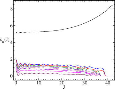
Figure 1: (Color online) The square roots of the eigenvalues of the matrix $S_{\alpha\beta}(J)$ for a single $j$–shell with $j=19/2$ and $m=6$ identical nucleons versus total spin $J$.

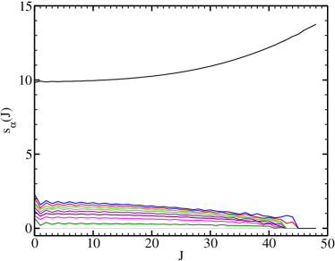
Figure 2: (Color online)Same as Fig. 1 but for $m=8$ nucleons.

Some of these features can be understood analytically via arguments presented in Appendix 4. We use the numerically established near independence of the largest eigenvalue $s_{1}(J)$ and of the associated eigenfunction ${\cal O}_{1\alpha}(J)$ on $J$ to study the average $X_{\alpha\beta}$ of $S_{\alpha\beta}$ (averaged over all $J$–values). We do so in the limit $(2j+1)\gg 1$. In this limit, $X_{\alpha\beta}$ factorizes, $X_{\alpha\beta}\approx f(\alpha)f(\beta)$. Hence all eigenvalues but one vanish, and $s^{2}_{1}$ is given by $\sum_{\alpha}f^{2}(\alpha)$. For $m=6$ ($m=8$) this yields $s_{1}\approx 6.3$ ($s_{1}\approx 11.4$, respectively). We also determine the eigenfunction ${\cal O}_{1\alpha}$ which (except for normalization) has components $(1,5,9,\ldots)$. The resulting matrix $B_{1}$ is

$$B_{1}\propto\sum_{s}(2s+1)C({\bf J},1+s/2)\ .$$ (12)

The sum runs over $s=0,2,4,\ldots,2j-1$ for the values of the two–particle spin. The matrix $B_{1}$ is the matrix of the monopole operator ${\cal B}_{1}$. Inspection reveals that this operator is approximately proportional to the unit operator. Thus, all matrices that are orthogonal (under the trace) to $B_{1}$ must have approximately zero trace. Moreover, the leading term in the transformed Hamiltonian (9) is approximately a scalar. It defines the approximate value of the centroid of the eigenvalues and has presumably only a small influence on the spectral statistics. The value of the centroid is determined by the values of $s_{1}({\bf J})$ and of $w(1)$. The spectral statistics are largely determined by the remaining terms in $H$.

Our analytical results are mirrored in the numerical findings. Except for the largest $J$–values, the matrices $B(J,1)$ are close to the unit matrix in $d(J)$ dimensions. Comparison with Figs. 1 and 2 shows that the analytical results for the eigenvalues are semiquantitatively correct. For the eigenfunction ${\cal O}_{1\alpha}$ the numerical diagonalization for $m=6$ and $J=0$ yields an overlap of 0.97 with the analytical result.

We turn to the data for the $sd$–shell. Our calculations are partly based on the shell–model code Oxbash Ox . The square roots $s_{\alpha}(J)$ for ²⁰Ne are shown in Fig. 3, those for ²⁴Mg are shown in Fig. 4 The tendencies are qualitatively similar to those in the single $j$–shell. In ²⁰Ne, $s_{1}(J)$ is not larger than all other roots by as big a factor as in the single $j$–shell, or as in ²⁴Mg. This suggests that the clear separation of $s_{1}(J)$ from the rest of the roots requires a minimum number of nucleons. Indeed, in Appendix 4, the factorization of $X_{\alpha\beta}$ occurs only for $m\geq 4$, and $s_{1}$ grows with $m$ roughly like $m^{2}$. Thus, our results suggest a generic behavior for many nucleons in the shell. Again, we find that the leading matrix $B(J,1)$ is (except for a normalization factor) approximately equal to the unit matrix.

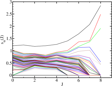
Figure 3: (Color online) The square roots of the eigenvalues of the matrix $S_{\alpha\beta}(J)$ for the $sd$–shell nucleus ²⁰Ne with isospin $T=0$ versus total spin $J$.

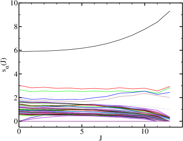
Figure 4: (Color online) Same as Fig. 3 but for ²⁴Mg.

Another remarkable feature in all the figures is the disappearance of one or several roots for some values of $J$. In fact, for each spin, at least one eigenvalue vanishes identically. The corresponding scalar two–body operator is given by ${\hat{J}}^{2}-J(J+1)$ where ${\hat{J}}$ denotes the operator of total spin. The matrix representation of this operators is a linear combination of the matrices $C_{\mu\nu}({\bf J})$. In the case of the $sd$–shell nuclei, an analogous statement applies to the isospin operator ${\hat{T}}^{2}-T(T+1)$. More eigenvalues than one vanish in cases where the number of independent matrix elements of $H({\bf J})$ is smaller than the number of two–body matrix elements.

How do these results relate to the actual determination of the effective shell model interaction from experimental data? We recall that usually one proceeds in two steps. In a first step, the effective interaction is determined through a $G$–matrix calculation that is based on nucleon–nucleon potentials which fit nucleon–nucleon scattering data with very high accuracy. The resulting $G$–matrix usually does not reproduce experimental nuclear spectra well enough, and corrections have to be made in a second step. There are basically two ways to make these corrections. A first approach insists on minimal corrections and only corrects the monopole term by a fit to experimental data. This is very reasonable since the monopole term has the largest trace norm, and is essentially the only matrix with a finite trace (or centroid). This last property of the monopole has been known since the pioneering work of Pasquini and Zuker Pas78 . We note that the resulting shell–model Hamiltonian has an impressive predictive power, see, e.g., the shell–model studies of $fp$–shell nuclei by the Strasbourg group Cau99 . In the second and alternative approach, one attempts to fit all two–body matrix elements to experimental data. This is done through an iterative procedure that starts from the $G$–matrix and makes small changes in the matrix elements until a best fit is obtained. As the number of data points (i.e., energy levels) usually exceeds the number of two–body matrix elements, the problem is over–determined, and only a smaller number of linear combinations of data points can be used in the fit due to rank–deficiency problems of the matrix equations involved Hon02 . As an example we mention the widely used Brown–Wildenthal interaction Bro88 for $sd$–shell nuclei where only 47 linear combinations of the 66 parameters (63 two–body matrix elements and three single–particle energies) are determined by fit while the remaing ones are taken from the $G$–matrix. In larger model spaces the ratio of well–determined linear combinations usually decreases. For the $fp$–shell, only 70 linear combinations out of 199 free parameters are used in the fit to data Hon04 . As shown by our results in this Subsection, the answer to the question “Which are the most important linear combinations of two–body matrix elements” is less determined by the data used in the fit but rather by the inherent structure of the shell model itself. Our work identifies which linear combinations these are: The $w_{\alpha}({\bf J})$’s which correspond (for fixed ${\bf J}$) to the largest eigenvalues. Unfortunately, the property of an eigenvalue to be large or small changes little (if at all) with ${\bf J}$, and the same is true of the orthogonal transformation defining the random variables $w_{\alpha}({\bf J})$. This fact shows that even an enlarged data set might not necessarily lead to more accurate values for the $w_{\alpha}({\bf J})$’s.

In conclusion, the information content of a nuclear spectrum as given by the TBRE is very different from that of a GOE. The actual possibility to determine the unknown parameters $w_{\alpha}({\bf J})$ depends on the magnitudes of the eigenvalues $s^{2}_{\alpha}({\bf J})$. We stress that these eigenvalues are uniquely determined by the underlying shell model and do not depend upon the residual interaction. Thus, they may be calculated prior to any attempt to fit the residual interaction to actual data. We believe that such a procedure might be useful for practical shell–model work.

III.2 Preponderance of Ground States with Spin Zero

In 1998, Johnson, Bertsch, and Dean JBD found that the TBRE is likely to yield spin–zero ground states in even–even nuclei with a probability which is considerably larger than the fraction of states with spin zero in the total shell–model space. This came as a surprise because the TBRE does not have a built–in pairing force or quadrupole force. Subsequent work showed that similar regularities exist in bosonic BiF and electronic JS many–body systems with two–body interactions. The phenomenon of spin–zero preponderance seems a robust and rather generic feature which has received much attention since, see the reviews ZV ; ZAY and references therein. Here we discuss it in the framework of our representation (9) of the Hamiltonian of the TBRE. We extend our earlier work in Ref. PW1 . As before in this paper, we focus attention on the case of a single $j$–shell and on the $T=0$ states of nuclei in the $sd$–shell and, therefore, use the label $J$ rather than ${\bf J}$.

Our approach is based upon the following consideration. For each value of $J$ and each realization of the random variables $v_{\alpha}$, we define the spectral radius $R(J)$ as the distance of the farthest eigenvalue from the center of the spectrum. (This can be the smallest or the largest eigenvalue. In view of the randomness of the signs of the $w_{\alpha}(J)$’s, that ambiguity is irrelevant). The $R(J)$’s are random variables. For every value of $J$ we determine the probability that the spectral radius $R(J)$ is maximal. To this end we relate $R(J)$ to the spectral width $\sigma(J)$. The square of the spectral width $\sigma(J)$ is given by the normalized trace norm of the Hamiltonian, see Eq. (11),

$$\sigma^{2}(J)=\sum_{\alpha=1}^{a_{1}}w^{2}_{\alpha}(J)s^{2}_{\alpha}(J)\ .$$ (13)

We postulate a linear relationship between the spectral radius and the spectral width,

$$R(J)=r(J)\sigma(J)\ .$$ (14)

We show that the scaling factors $r(J)$ are nearly constant (i.e., independent of the random variables $w_{\alpha}(J)$) but do depend upon $J$. Then, Eq. (14) relates the random variables $R(J)$ with the random variables $\sigma(J)$. The dependence of the scaling factors $r(J)$ on $J$ and the distribution of and correlations among the spectral widths $\sigma(J)$ together lead to an understanding of the preponderance of spin–zero ground states.

We first address the scaling factors $r(J)$. The inset of Fig. 5 shows the dependence of $R(0)$ on $\sigma(0)$ for 6 identical nucleons in the $j=19/2$ shell, together with a linear fit, for 900 realizations of the TBRE. We see that Eq. (14) holds with an approximately constant value of $r(0)$. The reduced $\chi^{2}$ per degree of freedom is about 0.9. This value increases toward 1.5 for spins around $J\approx 20$. Figure 5 shows the linear–fit values of $r(J)$ versus $J$. These have an overall tendency to decrease with increasing $J$. This fact reflects the overall decrease of the number $d(J)$ of states of spin $J$ with increasing $J$. Indeed, the smaller the number of states in the spectrum the closer do we expect $R(J)$ and $\sigma(J)$ to be. This expectation can be quantified. We recall that a shell–model spectrum with spin $J$ calculated from the TBRE has approximately Gaussian shape MF . For a Gaussian spectrum with spectral width $\sigma$ normalized to the total number $d$ of states, the average level density $\rho(E)$ has the form

$$\rho(E)=\frac{d}{\sqrt{2\pi}\sigma}\exp(-E^{2}/(2\sigma^{2}))\ .$$ (15)

The most likely position of the lowest (the highest) state in the spectrum is found by integrating $\rho(E)$ from $-\infty$ ($+\infty$, respectively) to the point where the area under the integral equals $1/2$. This point is equal to $R$. Thus,

$$\frac{1}{2}=\frac{d}{\sqrt{2\pi}}\int_{-\infty}^{-R/\sigma}{\rm d}x\exp(-x^{2}/2)\ .$$ (16)

The solutions $R/\sigma=r(d)$ of this equation depend on $d$. In Figure 5, we have displayed the resulting values for $r(d(J))$, again for the $j=19/2$ shell with $m=6$ identical nucleons. The odd–even staggering reflects corresponding changes in the dimensions $d(J)$. The error in our theoretical determination is expeced to be of the order of the mean level spacing, i.e., of order $d^{-1}$ and, thus, small for $d\gg 1$. The actual discrepancy between the data and our analysis is much larger. We ascribe this to the fact that the assumed Gaussian shape of the spectrum holds only approximately.

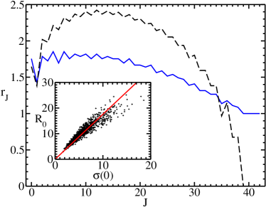
Figure 5: (Color online) Dependence of the scaling factor $r(J)$ in Eq. (14) on spin $J$ for $m=6$ identical nucleons in the $j=19/2$ shell. Solid line: Data based on the linear fit. Dashed line: Prediction based on Eq. (16). Inset: Dependence of $R(0)$ on $\sigma(0)$ for 900 random realizations of the TBRE. Solid line: The linear fit which determines $r(0)$.

We turn to the distributions of and the correlations among the spectral widths $\sigma(J)$. From Eq. (13), the ensemble average (henceforth denoted by an overbar) of $\sigma^{2}(J)$ is

$$\overline{\sigma^{2}(J)}=\sum_{\alpha=1}^{a_{1}}s^{2}_{\alpha}(J)\ ,$$ (17)

and the variance is

$$\overline{\sigma^{4}(J)}-\bigg{(}\overline{\sigma^{2}(J)}\bigg{)}^{2}=2\sum_{\alpha=1}^{a_{1}}s^{4}_{\alpha}(J)\ .$$ (18)

The normalized root of the variance equals $\sqrt{2/a_{1}}$ when all eigenvalues are equal and equals $\sqrt{2}$ when all eigenvalues but one vanish. Therefore, we conclude from Figures 1 to 4 that the fluctuations of $\sigma^{2}(J)$ are biggest for the largest $J$–values. This is also borne out when we calculate the complete probability distribution $P_{J}(\sigma)=2\sigma\overline{\delta(\sigma^{2}-\sigma^{2}(J))}$ for $\sigma(J)$. We write the $\delta$–function as a Fourier integral and perform the integrations over all the Gaussian variables $w_{\alpha}(J)$. We find

$$P_{J}(\sigma)=\frac{\sigma}{\pi}\int_{-\infty}^{+\infty}{\rm d}t\ e^{it\sigma^{2}}\ \prod_{\alpha=1}^{a_{1}}\frac{e^{-\frac{i}{2}{\rm arctan}(2ts^{2}_{\alpha}(J))}}{(1+4t^{2}s^{4}_{\alpha}(J))^{1/4}}\ .$$ (19)

Plots of $P_{J}(\sigma)$ for various values of $J$ were shown in Figure 3 of Ref. PW1 . The flattest curve is the one for the largest value of $J$ as expected.

Central to an understanding of the preponderance of spin–zero ground states in nuclei are the correlations between the spectral widths $\sigma(J)$ pertaining to different values of $J$. We have seen that both the eigenfunction pertaining to the largest eigenvalue and all eigenvalues of the matrix $S_{\alpha\beta}$ change little with $J$. In the extreme case where for a pair $(J,J^{\prime})$ of spins we would have $s^{2}_{\alpha}(J)=s^{2}_{\alpha}(J^{\prime})$ and $w_{\alpha}(J)=w_{\alpha}(J^{\prime})$ for all values of $\alpha$, the spectral widths would obviously be totally correlated: Their joint probability distribution is proportional to a delta function $\delta(\sigma(J)-\sigma(J^{\prime}))$. In this case, the value of the level with the lowest spin depends not on $\sigma(J)$ but only on $r(J)$. Actually the eigenvalues are not exactly equal and, more importantly, the eigenfunctions for the smaller eigenvalues differ, and so do the corresponding $w_{\alpha}(J)$’s. Still, we must expect significant correlations.

The correlations cannot be worked out directly from Eq. (13) as this would require knowledge of the correlations among the $w_{\alpha}(J)$’s for different values of $J$. Rather, we use that $\sigma^{2}$ is defined in terms of the trace norm of the Hamiltonian, use Eq. (2) for the latter and the definition (3) for $S_{\alpha\beta}(J)$ and have

$$\sigma^{2}(J)=\sum_{\alpha\beta}v_{\alpha}v_{\beta}S_{\alpha\beta}(J)\ .$$ (20)

For the covariance of two $\sigma^{2}$’s this yields

$$\overline{\sigma^{2}(J)\sigma^{2}(J^{\prime})}-\overline{\sigma^{2}(J)}\ \overline{\sigma^{2}(J^{\prime})}=2\ {\rm Trace}[S(J)S(J^{\prime})]\ .$$ (21)

In general, the right–hand side of this equation differs from zero. It is not possible straightforwardly to calculate the joint probability distribution of $\sigma(J)$ and $\sigma(J^{\prime})$. However, the probability

$$p(J,J^{\prime})=\overline{\Theta(\sigma^{2}(J)-\sigma^{2}(J^{\prime}))}$$ (22)

that spin $J$ has larger spectral width than spin $J^{\prime}$ can be calculated in terms of the eigenvalues $q_{\alpha}$ of the matrix $(S_{\alpha\beta}(J)-S_{\alpha\beta}(J^{\prime}))$. The calculation is quite similar to the one which leads to Eq. (19) and yields

$$p(J,J^{\prime})=\frac{1}{2}+\frac{1}{\pi}\int_{0}^{\infty}\frac{{\rm d}t}{t}\frac{\sin(\frac{1}{2}\sum_{\beta}\arctan 2tq_{\beta})}{\prod_{\alpha}(1+4t^{2}q^{2}_{\alpha})^{1/4}}\ .$$ (23)

This formula is in good agreement with our numerical results.

We emphasize that our approximations for $r(J)$ and $\sigma(J)$ do not yield a faithful representation of the distributions and correlations of the spectral radii $R(J)$. However, these approximations turn out to be sufficiently accurate to predict the probability that $R(J)=r(J)\sigma(J)$ has maximum value. These predictions are compared with the results of numerical diagonalization in Figs. 6 to 9. In all four Figures, we plot the probability that the ground state has spin $J$ versus $J$. The data points are calculated from 900 realizations of the TBRE. The solid lines show the probability that the spectral width $\sigma(J)$ has the largest value. The dashed lines show the probability that the product $r(J)\sigma(J)$ has the largest value.

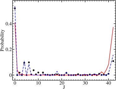
Figure 6: (Color online) The probability that the ground state has spin $J$ versus $J$ for $m=6$ identical nucleons in the $j=19/2$ shell. Dots: Data points from 900 realizations. Solid line: Probability that the spectral width $\sigma(J)$ has the largest value. Dashed line: Probability that the product $r(J)\sigma(J)$ has the largest value.

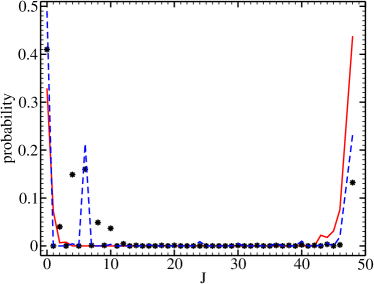
Figure 7: (Color online) Same as Fig. 6 but for $m=8$ identical nucleons

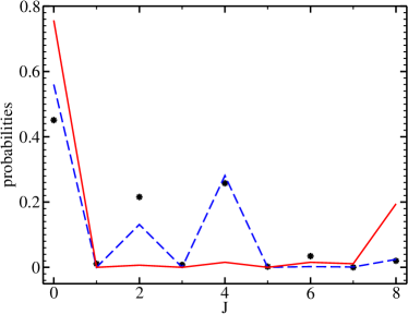
Figure 8: (Color online) Same as Fig. 6 but for the $T=0$ states in ²⁰Ne.

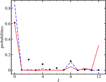
Figure 9: (Color online) Same as Fig. 6 but for the $T=0$ states in ²⁴Mg.

We observe that the states with spin zero and with maximum spin have the largest spectral widths. The factor $r(J)$ suppresses the high $J$–values. It causes a staggering in the probabilities which is not present for the spectral widths. In all Figures, the agreement of the dashed lines with the data points is satisfactory. We note that the predictions are somewhat less accurate for ²⁴Mg. A more detailed analysis of this case shows that the determination of the scale factor $r(J)$ by fit is somewhat less accurate as the typical $\chi^{2}$ per datum is around 2.5.

It is of some interest to see whether our arguments apply also to nuclei with an odd number of nucleons and half–integer total spin. In complete analogy to Figs. 6 to 9, we have calculated the probabilities for the half–integer spin states for $m=7$ identical nucleons in the single $j=19/2$ shell, to form the ground state. The results are shown in Fig. 10, with symbols that carry the same meaning as before. Again, the agreement is very convincing. This strengthens our belief that our approach is generic.

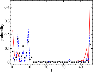
Figure 10: (Color online) Same as Fig. 6 but for $m=7$ identical nucleons

In summary, we have shown that our semi–analytical approach to the TBRE offers a satisfactory explanation for the preponderance of ground states with zero spin observed for this ensemble. We have established an approximate proportionality between two sets of random variables, the spectral radii $R(J)$ and the spectral widths $\sigma(J)$, $R(J)\approx r(J)\sigma(J)$, with nearly constant scaling factors $r(J)$. We have presented semi–analytical results for $r(J)$, and closed expressions for the distribution functions for the spectral widths as well as for some of their correlations and joint distribution functions. The scaling factors $r(J)$ depend essentially on the dimensions $d(J)$ of the associated Hilbert spaces, show odd–even staggering, and an overall decrease with increasing $J$. The spectral widths reflect properties of the underlying shell model and fluctuate most strongly for large values of $J$. Their average values are largest for $J=0$ and for maximum $J$. In the products $R(J)$, the large $J$–values are suppressed by the scaling factors $r(J)$. The good agreement of our theoretical predictions with the data in all cases suggests that we have identified the generic mechanism which is responsible for the preponderance of spin–zero ground states. That mechanism should likewise operate in other major shells and perhaps in other many–body systems governed by two–body interactions.

III.3 Correlations between Spectra with Different
Quantum Numbers and/or in Different Nuclei

For different quantum numbers ${\bf J}\neq{\bf J}^{\prime}$ and/or different nucleon numbers $m\neq m^{\prime}$, the Hamiltonian matrices of the TBRE defined in Eq. (2) depend upon the same set of random variables and are, therefore, correlated. This fact is rather obvious from the point of view of nuclear physics: Changing the residual interaction will simultaneously change all the spectra in all the nuclei within the major shell under consideration. However, from the point of view of random–matrix theory, the existence of correlations between spectra each of which displays Wigner–Dyson type level fluctuations, is excluded by assumption. To the best of our knowledge, a theoretical framework for the treatment of such correlations does not exist. The parametric level correlations which have been discussed earlier, in the context of both condensed–matter theory AS and random–matrix theory W , do not cover the present case. Indeed, there one considers a Hamiltonian which depends upon an external parameter like the strength of an external magnetic field. The dimension of the Hamiltonian matrix remains unchanged as the parameter is varied. Here, in contradistinction, correlations exist between Hamiltonian matrices which differ in matrix dimension. Moreover, parametric level correlations generically tend to zero as the difference between the old and the new values of the parameter increases. In the present case, it is not clear whether the correlation between two spectra differing, say, by two units of total spin is larger or smaller than that between two spectra differing by ten units. Also, it is not clear whether such correlations are big enough to be significant experimentally. These facts prompt us to explore the magnitude of spectral correlations both versus spin and versus mass. We focus attention on the case of $sd$–shell nuclei.

Using the standard definition for the level density

$$\rho(E,J)=\sum_{\mu}\delta(E-E_{\mu}(J))$$ (24)

in terms of the eigenvalues $E_{\mu}(J)$ pertaining to spin $J$, we have calculated numerically the density–density correlations for ²⁴Mg for $T=0$ states with $J=0$ and $J=1$. Our ensemble average uses 400 realizations of the TBRE. The results are shown in Fig. 11. The left panel shows as a density plot the mean value of the product of the level densities, $\overline{\rho(E,0)\rho(W,1)}$, versus the energies $E$ and $W$ in units of $v^{-2}$. The midddle panel shows analogously the product of the mean densities $\overline{\rho(E,0)}$ $\times$ $\overline{\rho(W,1)}$. This is essentially the product of two Gaussian distributions. The right panel shows the actual correlator, i.e., the difference $\overline{\rho(E,0)\rho(W,1)}-\overline{\rho(E,0)}\times\overline{\rho(W,1)}$. The maximum value of the correlator is about 10% of the product of the mean level densities. This demonstrates the existence of weak correlations. The correlator has a minimum in the center of the two spectra. We cannot exclude the possibility that with increasing matrix dimension, this minimum widens, so that significant correlations would exist only in the tails of the spectra. We have found correlations between spectra pertaining to different $J$–values also in the case of a single $j$-shell, where they are significantly stronger and are of the order of 50%. Correlations are also expected to exist between states in different nuclei when these are governed by the same TBRE. A case in point are the $T=0$ spin zero states in ²⁰Ne and ²⁴Mg. Their correlations are shown in Figure 12 where we use the same display as in Figure 11. Again, we find weak correlations of the order of several percent.

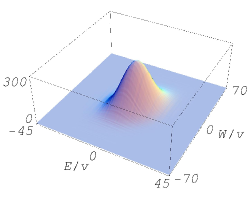
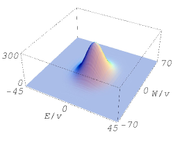
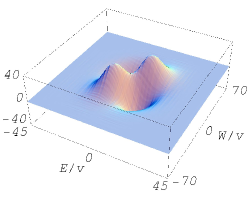
Figure 11: Correlations between the $J=0,T=0$ states and the $J=1,T=0$ states of ²⁴Mg (from 400 realizations of the ensemble). Left panel: Average of the product of the two level densities. Middle panel: Product of the averages of the two level densities. Right panel: The correlator.

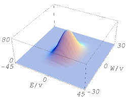
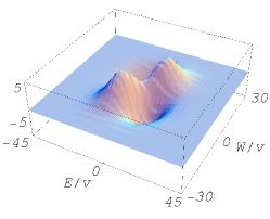
Figure 12: Same as Fig. 11 but for the $J=0,T=0$ states of ²⁴Mg and of ²²Ne (from 400 realizations of the ensemble).

In view of the results in Subsection III.1 and in Appendix 3, the existence of density–density correlations is expected. Indeed, the form (45) of the TBRE Hamiltonian shows that the centroids of the spectra must show particularly strong correlations. It is essentially these correlations that are displayed in Figs. 11 and 12. We ask: Are there also significant correlations between the spectral fluctuations of levels with different spins and/or different masses? These would show up in correlations between level spacings and would, thus, be independent of the fluctuations of the centroids of the spectra. To answer this question, a finer test than displayed in Figs. 11 and 12 is required. We have not explored this question any further. We recall, however, that data relevant to this question were published in Ref. JBD : With $E_{J}$ the energy of the lowest state with spin $J$, the ratio $\rho=(E_{4}-E_{2})/(E_{2}-E_{0})$ shows a broad peak in the range $\rho=0$ to $\rho\approx 1$. This suggests the existence of level correlations which go beyond those due to the centroids.

As remarked above, spectral fluctuations of spectra with different quantum numbers go beyond the assumptions of canonical random–matrix theory. Therefore, it would be of interest to verify the existence of such correlations experimentally. We have explored the possibility of such a test in the following way. In nuclei the residual interaction is fixed and not random. Therefore, ensemble averages cannot be taken. In canonical random–matrix theory, one circumvents this problem using ergodicity: The running average of an observable over a single realization of a spectrum is equal to its ensemble average. In the TBRE, we propose to take the average over an ensemble of nuclei in the same shell as a substitute. In the spirit of this proposal (which unfortunately lacks a theoretical foundation) we have calculated the spacings between the lowest levels for a number of $sd$–shell nuclei using the Brown-Wildenthal two–body interaction Bro88 . The ensemble consists of the nuclei ^20-24Ne, ^22-24Na, ^24-26Mg, ²⁶Al, ³⁰Si, ³⁴P, ^32,34S, and ³⁶Ar. For the even (odd) mass nuclei of this ensemble we considered the correlations of the $J=0$ and $J=2$ ($J=1/2$ and $J=5/2$) states. We label the nearest-neighbor spacings of levels with equal spins consecutively by $\Delta E_{i}$, $i=1,2,3,...$, starting from the ground state. Figure 13 shows, from left to right, the average of the spacings $\overline{\Delta E_{i}\Delta E_{j}}$, the product of the averages $\overline{\Delta E_{i}}\,\overline{\Delta E_{j}}$, and the correlator $\overline{\Delta E_{i}\Delta E_{j}}-\overline{\Delta E_{i}}\,\overline{\Delta E_{j}}$, in units of (MeV)². We see that correlations exist that are about 10% of the product of the averages.

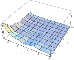
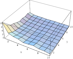
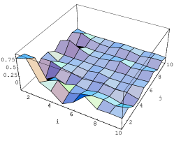
Figure 13: Level spacing correlations for 17 $sd$-shell nuclei between spins $J=0$ and $J=2$ ($J=1/2$ and $J=5/2$ )for even-$A$ (odd-$A$) nuclei. Left: Average of product of spacings. Middle: Product of average spacings; Right: Correlation.

The results of this subsection show that small correlations (of the order of 10%) exist between the spectral fluctuations of $sd$-shell nuclei. We expect that the experimental verification of the existence of these correlations is somewhat challenging, as it requires the measurement of several complete spectral sequences involving 5-10 levels each.

IV Summary

We have studied various aspects of the two–body random ensemble in nuclei, and presented three main results. First, the geometric properties of the nuclear shell model become transparent once one replaces the usual two–body operators by linear combinations that are orthogonal under the trace. This transformation yields one operator that is approximately proportional to the unit matrix and has the dominant spectral width. This monopole operator sets the scale for nuclear binding, and can be derived analytically. The remaining linear combinations of two–body operators have approximately zero centroid and smaller spectral widths. They determine the spectral fluctuation properties. Some of these operators have very small or even zero widths and therefore are close to or equal to the null operator. It is difficult or impossible to determine the corresponding linear combinations of two–body matrix elements by fit to experimental data. Thus, the geometric properties of the shell model explain the difficulties encountered when residual interactions are determined by fit.

Second, we presented analytical and numerical results regarding the fluctuations of and correlations between the spectral widths of shell–model operators. The total spectral width can be linked to the spectral radius through a simple scale factor. This approach allowed us to give a semi–quantitative explanantion for the preponderance of spin–zero ground states both for a single $j$–shell and for the $sd$–shell.

Third, we studied correlations between spectral fluctuations of spectra belonging to different spins and/or mass numbers. Our numerical results for the $sd$–shell indicate that correlations exist at the 10% level in the region of low–lying excitations. This is new territory and goes beyond the assumptions of canonical random–matrix theory. It would be of considerable interest to explore how these correlations depend on matrix dimension and, thus, change as we consider other major shells.

We have shown that the complex geometric structure of the shell model can be understood in rather simple terms. Apart from their theoretical interest, our results might be of practical use in fitting effective interactions, and they may motivate an experimental test of the correlations between spectra belonging to different quantum numbers.

Appendix 1. Two–body Interaction

For simplicity of notation, we confine ourselves to the case of a single $j$–shell and identical nucleons, omitting isospin and parity quantum numbers. The generalization is straightforward.

Let $a^{\dagger}_{\mu}$ and $a_{\mu}$ be the creation and annihilation operators for a particle with half–integer total spin $j$ and $z$–component $\mu$. Two such identical particles are coupled to total spin $s$ with $s=0,2,\ldots,2j-1$,

$$A^{s}_{M}=\sum_{\mu}c(jjs;\mu,M-\mu)a_{\mu}a_{M-\mu}\ .$$ (25)

This is a tensor of rank $s$ which is non–zero if $s$ is even. It transforms under rotations with the complex conjugate Wigner $D$–function,

$$(A^{s}_{M})_{new}=\sum_{N}(D^{s}_{MN})^{*}(A^{s}_{N})_{old}\ .$$ (26)

The adjoint operator is

$$(A^{s}_{M})^{\dagger}=-\sum_{\mu}c(jjs;\mu,M-\mu)a^{\dagger}_{\mu}a^{\dagger}_{M-\mu}\ .$$ (27)

This operator transforms with the usual $D$–function,

$$(A^{s}_{M})_{new}=\sum_{N}(D^{s}_{MN})(A^{s}_{N})_{old}\ .$$ (28)

From the unitarity of the $D$–functions, it follows that

$$T(s)=\sum_{M}(A^{s}_{M})^{\dagger}A^{s}_{M}$$ (29)

is a scalar.

It is convenient to rearrange the order of the creation and annihilation operators,

$$T(s) = -\sum_{\mu M\nu}c(jjs;\mu,M-\mu)c(jjs;\nu,M-\nu)$$ (30)

$$\times a^{\dagger}_{M-\mu}a_{\nu}a^{\dagger}_{\mu}a_{M-\nu}$$

$$+\sum_{\mu M}c^{2}(jjs;\mu,M-\mu)a^{\dagger}_{M-\mu}a_{M-\mu}$$

$$= -\sum_{\mu M\nu}c(jjs;\mu,M-\mu)c(jjs;\nu,M-\nu)$$

$$\times a^{\dagger}_{M-\mu}a_{\nu}a^{\dagger}_{\mu}a_{M-\nu}$$

$$+\frac{2j+1}{2s+1}\sum_{\mu}a^{\dagger}_{\mu}a_{\mu}\ .$$

With $m$ the number of particles in the shell, the last term is equal to $m(2j+1)/(2s+1)$. This term is denoted by $A(s)$ and gives a diagonal contribution to the Hamiltonian. We define the tensor operators ${\cal A}^{t}$ of rank $t$

$${\cal A}^{t}_{M}=\sum_{\rho}c(jjt;\rho,M-\rho)a^{\dagger}_{\rho}a_{\rho-M}\ .$$ (31)

For $t=0$, the tensor operator ${\cal A}^{t}$ is just the number operator, for $t=1$, it is the operator of total spin, etc. Using standard transformations of the Clebsch–Gordan coefficients, we rewrite the terms in Eq. (26) as

$$T(s) = (2s+1)\sum_{t}W(jjjj;st)\sum_{M}(-)^{s+2j+M}{\cal A}^{t}_{M}{\cal A}^{t}_{-M}$$ (32)

$$+A(s)\ .$$

With these definitions and with $\alpha=1+s/2$, the two–body interaction $V_{2}$ has the form

$$V_{2}=\sum_{\alpha=1}^{j+1/2}v_{\alpha}T(\alpha)$$ (33)

where we use either the definition (29) or the definition (32) for $T(s)$.

Appendix 2. Some properties of the matrices $C_{\mu\nu}({\bf J})$

As in Appendix 1, we confine ourselves to the case of a single $j$–shell and identical nucleons, omitting isospin and parity quantum numbers. We use the definition (25) and (27).

To work out the properties of the matrices $C_{\mu\nu}({\bf J})$, we shall presently need the commutator $[T(s),T(t)]$ for $s\neq t$, with $T(s)$ defined in Eq. (29). That commutator is given by

$$[T(s),T(t)] = \sum_{M,N}\bigg{(}(A^{s}_{M})^{\dagger}[A^{s}_{M},(A^{t}_{N})^{\dagger}]A^{t}_{N}$$ (34)

$$\qquad+(A^{t}_{N})^{\dagger}[(A^{s}_{M})^{\dagger},A^{t}_{N}]A^{s}_{N}\bigg{)}\ .$$

The commutator of two $A$’s can be expressed in terms of the irreducible tensor operators ${\cal A}$ introduced in Eq. (31). We find

$$[(A^{s}_{M})^{\dagger},A^{t}_{N}] = -4\sum_{p}\sqrt{(2s+1)(2p+1)}W(sjtj;jp)$$ (35)

$$\times c(stp;M,N)B^{p}_{M-N}\ .$$

Here $B^{p}_{m}$ is an irreducible tensor of rank $p$ defined as

$$B^{p}_{m}=\sum_{n}(-)^{j-n}c(jjp;-n,n-m)a^{\dagger}_{n}a_{n-m}\ .$$ (36)

Hence,

$$[T(s),T(t)] = -\sum_{p}\sqrt{\frac{(2s+1)(2p+1)}{2t+1}}W(sjtj;jp)$$

$$\qquad\times\sum_{M,N}c(stp;M,N)(A^{t}_{N})^{\dagger}B^{p}_{M-N}A^{s}_{M}$$

$$+\sum_{p}\sqrt{\frac{(2t+1)(2p+1)}{2s+1}}W(tjsj;jp)$$

$$\qquad\times\sum_{M,N}c(tsp;N,M)(A^{s}_{M})^{\dagger}B^{p}_{N-M}A^{t}_{M}\ .$$

The result is a scalar because the three operators $A^{\dagger},B$ and $A$ are coupled to rank zero. It is obvious that the commutator $[T(s),T(t)]$ differs from zero and does not lie in the linear space spanned by the operators $T$. A recoupling of the operators shows, in fact, that the commutator is a sum of three–body operators.

The elements of the matrices $C_{\mu\nu}(J,s)$ with $s=2\alpha-2$, may be viewed as matrix elements of operators ${\cal C}(J,s)$. The latter are defined in the space of Slater determinants of single–particle shell–model states (i.e., states not coupled to total spin $J$) and have the form

$${\cal C}(J,s)={\cal P}(J)T(s){\cal P}(J)$$ (38)

where ${\cal P}(J)$ is the orthonormal projector onto the subspace of many–body states with fixed total spin $J$. The projectors obey

$${\cal P}(J_{1}){\cal P}(J_{2})={\cal P}(J_{1})\delta_{J_{1}J_{2}}\ ;\ [{\cal P}(J)]^{\dagger}={\cal P}(J)\ .$$ (39)

With the help of the operator ${\vec{J}}$ of total spin, ${\cal P}(J)$ is explicitly written as

$${\cal P}(J)=\prod_{J_{l}\neq J}\frac{{\vec{J}}^{2}-J_{l}(J_{l}+1)}{J(J+1)-J_{l}(J_{l}+1)}\ .$$ (40)

The multiplication extends over all possible values $J_{l}$ of total spin.

It is straightforward to show that the operators ${\cal P}(J)$ commute with $T(s)$. Therefore, we have

$${\cal C}(J,s)={\cal P}(J)T(s){\cal P}(J)=T(s){\cal P}(J)={\cal P}(J)T(s)\ .$$ (41)

It follows that the commutator $[{\cal C}(J,s),{\cal C}(J,t)]$ can be written as

$$[{\cal C}(J,s),{\cal C}(J,t)]={\cal P}(J)[T(s),T(t)]\ .$$ (42)

But we have shown in Eq. (LABEL:B4) that the commutator $[T(s),T(t)]$ does not vanish and is, in fact, a sum of three–body operators. It then follows from Eq. (42) that the operators ${\cal C}$ do not commute. Rather, their commutators represent sums of three–body operators (projected, of course, onto the space with fixed $J$). In particular, it is not possible to diagonalize the ${\cal C}$’s simultaneously.

Appendix 3. Another Form of the TBRE

As mentioned in Subsection III.1, there exists another possibly useful form of the TBRE. This we now derive. For $\alpha=1,\ldots,a$ we define

$$c({\bf J},\alpha)={\rm Trace}\ C_{\mu\nu}({\bf J},\alpha)$$ (43)

and introduce the traceless matrices

$${\tilde{C}}_{\mu\nu}({\bf J},\alpha)=C_{\mu\nu}({\bf J},\alpha)-\frac{c({\bf J},\alpha)}{d({\bf J})}\delta_{\mu\nu}\ .$$ (44)

With these definitions, the Hamiltonian in Eq. (2) takes the form

$$H_{\mu\nu}({\bf J})={\tilde{H}}_{\mu\nu}({\bf J})+\bigg{(}\sum_{\alpha=1}^{a}\frac{c({\bf J},\alpha)}{d({\bf J})}v_{\alpha}\bigg{)}\delta_{\mu\nu}$$ (45)

where

$${\tilde{H}}_{\mu\nu}({\bf J})=\sum_{\alpha}v_{\alpha}{\tilde{C}}_{\mu\nu}({\bf J},\alpha)$$ (46)

is traceless. We can now diagonalize the real symmetric positive semidefinite $a$–dimensional matrix

$${\tilde{S}}_{\alpha\beta}=\frac{1}{d({\bf J})}{\rm Trace}\ [{\tilde{C}}({\bf J},\alpha){\tilde{C}}({\bf J},\beta)]$$ (47)

by an orthogonal transformation ${\tilde{\cal O}}_{\alpha\beta}({\bf J})$. Of the resulting eigenvalues ${\tilde{s}}^{2}({\bf J},\alpha)$, exactly $(a_{1}-1)$ differ from zero. Using the same construction as in Eqs. (4) to (8) and denoting the resulting $a_{1}-1$ orthonormal matrices by ${\tilde{B}}({\bf J},\alpha)$, we arrive at

$$H_{\mu\nu}({\bf J}) = \sum_{\alpha=1}^{a_{1}-1}{\tilde{w}}_{\alpha}({\bf J}){\tilde{s}}_{\alpha}({\bf J}){\tilde{B}}({\bf J},\alpha)$$ (48)

$$+ \delta_{\mu\nu}\sum_{\alpha=1}^{a}\frac{c({\bf J},\alpha)}{d({\bf J})}v_{\alpha}\ .$$

Similarly as in Eq. (10) but with ${\cal O}$ replaced by $\tilde{\cal O}$, the $(a_{1}-1)$ random variables ${\tilde{w}}_{\alpha}({\bf J})$ are linear combinations of the $v_{\alpha}$’s. They are uncorrelated, have mean values zero, and a common second moment equal to unity. The matrices ${\tilde{B}}({\bf J},\alpha)$ are traceless and, hence, orthogonal to the unit matrix in the sense of the trace norm. Thus, Eq. (48) is another representation of the TBRE in terms of $a_{1}$ orthonormal matrices. In contrast to Eq. (9), we have now separated a term (proportional to the unit matrix) which defines the centroid of the spectrum but has no bearing on the actual level sequence, from the remainder which in turn possesses a vanishing centroid but yields the actual details of the spectrum. The form (48) is probably not useful for data analyses but should be helpful whenever we are interested in spectral fluctuation properties. These depend only upon the $a_{1}-1$ variables ${\tilde{w}}_{\alpha}({\bf J})$.

Appendix 4. Approximate Diagonalization of $S_{\alpha\beta}$

As in previous Appendices, we perform the calculation for a single $j$–shell with identical nucleons. The number of nucleons is denoted by $m$. We use the fact that here we have $s=2\alpha-2$ and replace $\alpha,\beta$ by $s,t$. We use the definition (41) and the fact that $P(J)$ and $T(s)$ commute to write $S_{st}$ in the form

$$S_{st}(J)=\frac{1}{d(J)}{\rm Trace}\ [{\cal P}(J)T(s)T(t)]\ .$$ (49)

The calculation is difficult for fixed total spin $J$. However, our numerical calculations show that the eigenvalues of $S_{st}(J)$ and the eigenvector pertaining to the largest eigenvalue change little with $J$ for the lowest values of $J$. Moreover, these lowest values of $J$ have the largest values of $d(J)$. Therefore, we approximate the calculation of $S_{st}(J)$ by averaging over all values of $J$, thus defining

$$X_{st}=\frac{1}{\sum_{J}d(J)}\sum_{J}d(J)S_{st}(J)\ .$$ (50)

We observe that the sum over $J$ removes the projectors ${\cal P}(J)$ since their sum equals unity. Thus, the average is equal to the normalized trace of $T(sT(t)$ taken with respect to all states in the Hilbert space spanned by normalized Slater determinants (without any attention paid to the coupling of spins). We denote that trace by angular brackets and have

$$X_{st}=\langle T(s)T(t)\rangle\ .$$ (51)

We calculate $X_{st}$ approximately by keeping only the leading terms in an expansion in inverse powers of $(2j+1)$. That is the meaning of the approximate sign in this Appendix.

The trace in Eq. (51) can be worked out using Wick contraction. The relevant term is

$$\langle a^{\dagger}_{\mu}a^{\dagger}_{M-\mu}a_{\nu}a_{M-\nu}a^{\dagger}_{\rho}a^{\dagger}_{N-\rho}a_{\sigma}a_{N-\sigma}\rangle\ .$$ (52)

Two types of Wick contractions occur: (a) Those where contractions connect pairs of operators separately within the group of the first four and of the second four operators, and (b) those where at least two operators of the first group of four are contracted with the same number of operators of the second group. Among all these, the terms of leading order in an expansion in inverse powers of $(2j+1)$ are the terms with the maximum number of unconstrained summations over magnetic quantum numbers. Every Wick contraction of a pair of operators produces a Kronecker delta. However, the two Wick contractions in case (a) affecting the first (the second) group of four operators produce the same Kronecker delta’s $\delta_{\mu\nu}$ ($\delta_{\rho\sigma}$, respectively). This is not so in case (b) where each of the two Kronecker delta’s imposes a new constraint. We conclude that the terms of leading order arise only from Wick contractions for case (a). This fact implies that

$$X_{st}\approx\langle T(s)\rangle\ \langle T(t)\rangle=f(s)f(t)$$ (53)

where we have defined

$$f(s)=\langle T(s)\rangle\ .$$ (54)

Factorization of $X$ as in Eq. (53) implies that the leading eigenvalue $s^{2}_{1}$ defined in Eq. (4) is given by

$$s^{2}_{1}\approx\sum_{s}f^{2}(s)$$ (55)

while all other eigenvalues are $\approx 0$. The associated matrix $B_{1}$ is the matrix representation of an operator ${\cal B}_{1}$. The latter is proportional to $\sum_{s}f(s)T(s)$. Normalization requires $\langle B^{2}_{1}\rangle=1$. We use again that the Wick contractions approximately factorize and find that

$${\cal B}_{1}\approx\frac{1}{\sum_{s}f^{2}(s)}\ \sum_{s}f(s)T(s)\ .$$ (56)

We observe that $\langle B_{1}\rangle\approx 1$. The same statement holds, within our factorization approximation, for all higher powers of $B_{1}$. Thus, $B_{1}$ is (except for normalization) approximately equal to the unit matrix. With the dimension of total Hilbert space given by $N(j,m)={2j+1\choose m}$, this gives

$$B_{1}\approx N^{-1/2}(j,m)\ {\bf 1}\ .$$ (57)

It remains to work out the function $f(s)$. We denote the Wick contraction by an index $W$. We have

$$\bigg{(}a^{\dagger}_{\mu}a^{\dagger}_{M-\mu}a_{\nu}a_{M-\nu}\bigg{)}_{W}=[\delta_{\mu\nu}-\delta_{\mu M-\nu}]a^{\dagger}_{\mu}a^{\dagger}_{M-\mu}a_{\mu}a_{M-\mu}\ .$$ (58)

Thus,

$$f(s) = \langle T(s)\rangle\approx\sum_{M\mu\nu}c(jjs;\mu,M-\mu)c(jjs;\nu,M-\nu)$$ (59)

$$\times[\delta_{\mu\nu}-\delta_{\mu M-\nu}]\bigg{(}\frac{m}{2j+1}\bigg{)}^{2}$$

or

$$f(s)\approx\bigg{(}\frac{m}{2j+1}\bigg{)}^{2}\ 2\ (2s+1)\ .$$ (60)

For $j=19/2$ and $m=6$ ($m=8$), this yields for $s^{2}_{1}$ the value $39.933$ ($126.21$) so that $s_{1}=6.32$ ($11.24$, respectively).

With $f(s)$ given by Eq. (60), we can work out ${\cal B}_{1}$ explicitly using Eq. (56) and Eq. (30) for $T(s)$, omitting normalization factors. This yields

$${\cal B}_{1} \propto \frac{1}{(\sum_{s}(st+1)^{2})^{1/2}}\bigg{\{}\frac{1}{2}(2j+1)^{2}m\ {\bf 1}$$ (61)

$$-\sum_{sM\mu\nu}(2s+1)c(jjs;\mu,M-\mu)c(jjs;\nu,M-\nu)$$

$$\times a^{\dagger}_{M-\mu}a_{\nu}a^{\dagger}_{\mu}a_{M-\nu}\bigg{\}}\ .$$

We retrieve the unit matrix as in Eq. (57) and conclude that compared to the laeding term, the last sum in Eq. (61) is of order $1/(2j+1)$.

These results allow us to estimate $s^{2}_{1}(J)$. We do so by assuming that the results obtained by averaging over all values of $J$ apply separately to each $J$. Since $B(J,1)$ is, except for terms of order $1/(2j+1)$, equal to a multiple of the unit matrix, we equate the variance of the coefficient multiplying $B(J,1)$ in Eq. (9) with the variance of the coefficient multiplying $d^{-1/2}(J)\delta_{\mu\nu}$ in Eq. (48). We obtain

$$s^{2}_{1}(J)\approx(1/d(J))\sum_{\alpha}c^{2}(J,\alpha)\ .$$ (62)

By the same token, we expect that all the $a_{1}-1$ eigenvalues ${\tilde{s}}^{2}_{\alpha}(J)$ in Eq. (47) are on average of equal size and of order $1/(2j+1)$. This implies that the statistical fluctuations of the centroid of the spectrum are considerably larger than those of individual level spacings.

In summary, we have shown that the leading eigenvalue and eigenfunction of $X_{st}$ are easily obtained because for $2j+1\gg 1$, $X_{st}$ approximately factorizes. The factors $f(s)$ and $f(t)$ are simply given by Wick–contracting the operators $T(s)$ and $T(t)$ separately. The leading eigenvalue is given by Eq. (55) and the matrix $B_{1}$ is approximately given by the unit matrix.

This research was supported in part by the U.S. Department of Energy under Contract Nos. DE-FG02-96ER40963 (University of Tennessee) and DE-AC05-00OR22725 with UT-Battelle, LLC (Oak Ridge National Laboratory).

References

- (1) R. U. Haq, A. Pandey, and O. Bohigas, Phys. Rev. Lett. 48, 1086 (1982).
- (2) A. Y. Abul-Magd, H. L. Harney, M. H. Simbel, and H. A. Weidenmüller, Phys. Lett. B 579 278 (2004).
- (3) J. H. D. Jensen and M. Mayer, Elementary Theory of Nuclear Shell Structure, Wiley, New York 1955.
- (4) J. B. French and S. S. M. Wong, Phys. Lett. B 33, 449 (1970).
- (5) O. Bohigas and J. Flores, Phys. Lett. B 34, 261 (1971).
- (6) V. Zelevinsky, B. A. Brown, N. Frazier, and M. Horoi, Phys. Rep. 276, 85 (1996).
- (7) T. Papenbrock and H. A. Weidenmüller, Nucl. Phys. A 757, 422 (2005); nucl-th0403041.
- (8) T. Papenbrock and H. A. Weidenmüller, Phys. Rev. Lett. 93, 132503 (2004); nucl-th/0404022.
- (9) J. B. French, Phys. Lett. B 26, 75 (1967).
- (10) B. A. Brown, A. Etchegoyen, and W. D. M. Rae, The computer code OXBASH, MSU-NCSL report number 524, 1988.
- (11) E. Pasquini and A. P. Zuker, in Physics of Medium Light Nuclei, Florence, 1977, edited by P. Blasi and R. Ricci (Editrice Compositrice, Bologna, 1978).
- (12) E. Caurier, G. Martinez-Pinedo, F. Nowacki, A. Poves, J. Retamosa, and A. P. Zuker, Phys. Rev. C59, 2033 (1999); nucl-th/9809068.
- (13) M. Honma, B. A. Brown, T. Mizusaki, and T. Otsuka, Nucl. Phys. A 704, 134c (2002).
- (14) B. A. Brown and B. H. Wildenthal, Annu. Rev. Nucl. Part. Sci. 38, 29 (1988).
- (15) M. Honma, T. Otsuka, B. A. Brown, and T. Mizusaki, Phys. Rev. C69, 034335 (2004); nucl-th/0402079.
- (16) C. W. Johnson, G. F. Bertsch, and D. J. Dean, Phys. Rev. Lett. 80, 2749 (1998); nucl-th/9802066.
- (17) R. Bijker and A. Frank, Phys. Rev. Lett. 84, 420 (2000); nucl-th/9911067.
- (18) P. Jacquod and A. D. Stone, Phys. Rev. Lett. 84, 3938 (2000); cond-mat/9909067.
- (19) V. Zelevinsky and A. Volya, Phys. Rep. 391, 311 (2004); nucl-th/0309071.
- (20) Y. M. Zhao, A. Arima, and N. Yoshinaga, Phys. Rep. 400, 1 (2004), nucl-th/0311050.
- (21) K. K. Mon and J. B. French, Ann. Phys. (N.Y.) 95 90 (1975).
- (22) B. D. Simons and B. L. Altshuler, Phys. Rev. Lett. 70, 4063 (1993); Phys. Rev. B8, 5422 (1993).
- (23) H. A. Weidenmüller, J. Phys: Condens. Matter 17, S1881 (2005).