Chiral dynamics in the $\gamma p\to\pi^{0}\eta p$ and $\gamma p\to\pi^{0}K^{0}\Sigma^{+}$ reactions

Abstract

Using a chiral unitary approach for meson-baryon scattering in the strangeness zero sector, where the $N^{*}(1535)S_{11}$ resonance is dynamically generated, we study the reactions $\gamma p\to\pi^{0}\eta p$ and $\gamma p\to\pi^{0}K^{0}\Sigma^{+}$ at photon energies at which the final states are produced close to threshold. Among several reaction mechanisms, we find the most important is the excitation of the $\Delta^{*}(1700)D_{33}$ state which subsequently decays into a pseudoscalar meson and a baryon belonging to the $\Delta(1232)P_{33}$ decuplet. Hence, the reaction provides useful information with which to test current theories of the dynamical generation of the low-lying $3/2^{-}$ states. The first reaction is shown to lead to sizable cross sections and the $N^{*}(1535)S_{11}$ resonance shape is seen clearly in the $\eta p$ invariant mass distribution. The same dynamical model is shown to lead to much smaller cross sections at low energies in the second reaction. Predictions are made for cross sections and invariant mass distributions which can be compared with ongoing experiments at ELSA.

I Introduction

The unitary extensions of chiral perturbation theory $U\chi PT$ have brought new light in the study of the meson-baryon interaction and have shown that some well known resonances qualify as dynamically generated, or in simpler words, they are quasibound states of a meson and a baryon, the properties of which are described in terms of chiral Lagrangians. After early studies in this direction explaining the $\Lambda(1405)S_{01}$ and the $N^{*}(1535)S_{11}$ as dynamically generated resonances Kaiser:1995cy ; Kaiser:1996js ; kaon ; Nacher:1999vg ; Oller:2000fj , more systematic studies have shown that there are two octets and one singlet of resonances from the interaction of the octet of pseudoscalar mesons with the octet of stable baryons Jido:2003cb ; Garcia-Recio:2003ks . The $N^{*}(1535)S_{11}$ belongs to one of these two octets and plays an important role in the $\pi N$ interaction with its coupled channels $\eta N$, $K\Lambda$ and $K\Sigma$ Inoue:2001ip . In spite of the success of the chiral unitary approach in dealing with the meson-baryon interaction in these channels, the fact that the quantum numbers of the $N^{*}(1535)S_{11}$ are compatible with a standard three constituent quark structure and that its mass is roughly obtained in many standard quark models Isgur:1978xj ; Capstick:1993kb , or recent lattice gauge calculations Chiu:2005zc , has as a consequence that the case for the $N^{*}(1535)S_{11}$ to be described as a dynamically generated resonance appears less clean than that of the $\Lambda(1405)S_{01}$ where both quark models and lattice calculations have shown systematic difficultiesNakajima:2001js . Ultimately, it will be the ability of the models to describe different experiments in which the resonances are produced that will settle the issue of what represents Nature better at a certain energy scale. A detailed description of many such experiments has been discussed in review .

A good example is found in the recent experiment on photoproduction of the $\Lambda(1405)S_{01}$ resonance in the $\gamma p\to K^{+}\pi\Sigma$ reaction Ahn:2003mv , where theoretical predictions using the chiral unitary approach had been done previously Nacher:1998mi . In the present paper we adopt and extend the ideas of Nacher:1998mi and study the analogous reaction $\gamma p\to\pi^{0}\eta p$ where the $\eta p$ final state can form the $N^{*}(1535)S_{11}$ resonance. This reaction is currently being analyzed at ELSAMetag

Some of the reaction mechanisms in our model are described as a two-step process: In the initial photoproduction, two mesons are generated, one of which is the final $\pi^{0}$. The final state interaction of the other meson with the proton is then responsible for the $\eta$ production. For this interaction chiral Lagrangians in $SU(3)$ representation involving only mesons and baryons are used. In addition, the contributions from explicit baryonic resonance exchange such as $\Delta(1232)P_{33}$, $N^{*}(1520)D_{13}$, and $\Delta^{*}(1700)D_{33}$, which have been found essential for the two meson photoproduction, e.g., in the Valencia model Nacher:2000eq ; GomezTejedor:1993bq ; GomezTejedor:1995pe , will be included. The $\Delta^{*}(1700)D_{33}$ resonance, as recent studies show Kolomeitsev:2003kt ; Sarkar:2004jh , qualifies as dynamically generated through the interaction of the $0^{-}$ meson octet and the $3/2^{+}$ baryon decuplet . In this picture it is possible Sarkar:2004jh to obtain the coupling of the $\Delta^{*}(1700)D_{33}$ to the $\eta\Delta(1232)P_{33}$ and $K\Sigma^{*}(1385)P_{13}$ for which experimental information does not yet exist.

In Sec. II the model for the dynamical generation of the $N^{*}(1535)S_{11}$ resonance in $\pi N\to\pi N$ scattering will be briefly reviewed with special emphasis on the $\pi N\to\eta N$ transition. Subsequently, we study the one-meson photoproduction $\gamma p\to\eta p$ in Sec. II.1. This allows for a simultaneous description of the existing data for these three different reactions within the chiral model. In Sec. III we predict observables for the photoproduction of $\pi^{0}\eta p$ in the final state.

At the same time we also study the $\gamma p\to\pi^{0}K^{0}\Sigma^{+}$ reaction and make predictions for its cross section, taking advantage of the fact that it appears naturally within the coupled channels formalism of the $\gamma p\to\pi^{0}\eta p$ reaction and leads to a further test of consistency of the ideas explored here.

In this section we have referred to all resonances that will enter the evaluation of our amplitudes. In what follows for shortness of notation we will omit the description in terms of $L_{2I,2J}$.

II The $N^{*}(1535)$ in meson-baryon scattering

Before turning to the photoproduction reactions of the next sections, let us recall the properties of the $N^{*}(1535)$ in the meson-baryon sector, where this resonance shows up clearly in the spin isospin $(S=1/2,I=1/2)$ channel. In the past, this resonance has been proposed to be dynamically generated Kaiser:1995cy ; Kaiser:1996js ; Nacher:1999vg ; Inoue:2001ip rather than being a genuine three-quark state. The model of Ref. Inoue:2001ip provides an accurate description of the elastic and quasielastic $\pi N$ scattering in the $S_{11}$ channel. Within the coupled channel approach in the $SU(3)$ representation of Ref. Inoue:2001ip , not only the $\pi N$ final state is accessible, but also $K\Sigma$, $K\Lambda$, and $\eta N$ in a natural way.

In the case of the present reactions, we are interested in the $\eta p$ interaction which will manifest the $N^{\star}(1535)$ resonant character. This interaction was studied in detail in Ref. Inoue:2001ip for the charge $Q=0$, strangeness zero sector. In the present study we work in the charge $Q=+1$ sector, which requires the simultaneous consideration of the coupled channels

$$\pi^{0}p,\;\pi^{+}n,\;\eta p,\;K^{+}\Sigma^{0},\;K^{+}\Lambda,\;K^{0}\Sigma^{+}\;.$$ (1)

We will subsequently refer to these channels as one through six in the order given above. In this section we derive the necessary modifications of the coupled channels in the $Q=+1$ sector and briefly review the basic formalism. The theoretical framework of the photoproduction mechanisms is found in subsequent sections.

We thus begin with the lowest order chiral Lagrangian for the meson-baryon interaction ulf ; ecker

$${\cal L}_{1}^{(B)} = \left\langle\bar{B}i\gamma^{\mu}\nabla_{\mu}B\right\rangle-M_{B}\left\langle\bar{B}B\right\rangle$$ (2)

$$+\frac{1}{2}D\left\langle\bar{B}\gamma^{\mu}\gamma_{5}\left\{u_{\mu},B\right\}\right\rangle+\frac{1}{2}F\left\langle\bar{B}\gamma^{\mu}\gamma_{5}[u_{\mu},B]\right\rangle$$

where the symbol $\left\langle\right\rangle$ denotes the trace of SU(3) matrices and

$$\nabla_{\mu}B = \partial_{\mu}B+[\Gamma_{\mu},B],$$

$$\Gamma_{\mu} = \frac{1}{2}(u^{+}\partial_{\mu}u+u\partial_{\mu}u^{+}),$$

$$U = u^{2}={\rm exp}(i\sqrt{2}\Phi/f),$$

$$u_{\mu} = iu^{+}\partial_{\mu}Uu^{+}$$ (3)

with $\Phi$ and $B$ the usual $3\times 3$ $SU(3)$ matrices of the fields for the meson octet of the pion and the baryon octet of the nucleon, respectively ulf . The term with the covariant derivative $\nabla_{\mu}$ in Eq. (2) generates the Weinberg-Tomozawa interaction and leads to the lowest order transition amplitude

$$V_{ij}=-C_{ij}\;\frac{1}{4f_{i}f_{j}}\;\overline{u}(p^{\prime})\gamma^{\mu}u(p)(k_{\mu}+k_{\mu}^{\prime})$$ (4)

where $p,p^{\prime}$ ($k,k^{\prime}$) are the initial and final momenta of the baryons (mesons). The coefficients $C_{ij}$ are $SU(3)$ factors which one obtains from the Lagrangian, and the $f_{i}$ are the $\pi$, $\eta$, $K$ decay constants gasser . The $C_{ij}$ coefficients for the channels with charge +1 are shown in Tab. 1.

Table 1: $C_{ij}$ coefficients for the six channels. The matrix is symmetric.

	$\pi^{0}p$	$\pi^{+}n$	$\eta p$	$K^{+}\Sigma^{0}$	$K^{+}\Lambda$	$K^{0}\Sigma^{+}$
$\pi^{0}p$	$0$	$\sqrt{2}$	$0$	$-\frac{1}{2}$	$-\frac{\sqrt{3}}{2}$	$\frac{1}{\sqrt{2}}$
$\pi^{+}n$		$1$	$0$	$\frac{1}{\sqrt{2}}$	$-\sqrt{\frac{3}{2}}$	$0$
$\eta p$			$0$	$-\frac{\sqrt{3}}{2}$	$-\frac{3}{2}$	$-\sqrt{\frac{3}{2}}$
$K^{+}\Sigma^{0}$				$0$	$0$	$\sqrt{2}$
$K^{+}\Lambda$					$0$	$0$
$K^{0}\Sigma^{+}$						$1$

The amplitudes after unitarization are given in matrix form Inoue:2001ip by means of the Bethe-Salpeter equation

$$T(\sqrt{s})=\left[1-V(\sqrt{s})G(\sqrt{s})\right]^{-1}V(\sqrt{s})$$ (5)

with $V$ obtained from Eq. (4). We are only interested in the s-wave meson-baryon interaction to generate the $S_{11}$ amplitude; the projection of $V$ into this partial wave is given in ref. Inoue:2001ip , as well as $G$ which is the meson-baryon loop function in dimensional regularization. In the following we denote by $T^{(ij)}$ the matrix elements of $T$ with the channel ordering of Eq. (1).

A second modification of the model of Ref. Inoue:2001ip with respect to other approaches concerns the $\pi N\to\pi\pi N$ channel. This channel was important to obtain a good description of the $I=3/2$ amplitude but it has only a small influence in the $I=1/2$ channel. It increases the width by about 10 % and changes the position of the $N^{\star}(1535)$ by about 10 MeV. In the charge +1 sector this channel can be included by a change of the potential according to $V_{\pi N,\pi N}\to V_{\pi N,\pi N}+\delta V$ as in Ref. Doring:2004kt and reads:

$$\delta V(\pi^{0}p\to\pi^{0}p) = \left[\left(-\frac{\sqrt{2}}{3}\;v_{31}-\frac{1}{3\sqrt{2}}\;v_{11}\right)^{2}+\left(\frac{1}{3}\;v_{31}-\frac{1}{3}\;v_{11}\right)^{2}\right]G_{\pi\pi N}$$

$$\delta V(\pi^{0}p\to\pi^{+}n) = \Bigg{[}\left(-\frac{\sqrt{2}}{3}\;v_{31}-\frac{1}{3\sqrt{2}}\;v_{11}\right)\left(\frac{1}{3}\;v_{31}-\frac{1}{3}\;v_{11}\right)$$

$$+\left(\frac{1}{3}\;v_{31}-\frac{1}{3}\;v_{11}\right)\left(-\frac{1}{3\sqrt{2}}\;v_{31}-\frac{\sqrt{2}}{3}\;v_{11}\right)\Bigg{]}G_{\pi\pi N}$$

$$\delta V(\pi^{+}n\to\pi^{+}n) = \left[\left(\frac{1}{3}\;v_{31}-\frac{1}{3}\;v_{11}\right)^{2}+\left(-\frac{1}{3\sqrt{2}}\;v_{31}-\frac{\sqrt{2}}{3}\;v_{11}\right)^{2}\right]G_{\pi\pi N}$$ (6)

with the isospin classification and conventions as in Ref. Inoue:2001ip ; $G_{\pi\pi N}$ being the $\pi\pi N$ loop function that incorporates the two-pion relative momentum squared. Analytic expressions for $v_{11}$ and $v_{31}$ are found in Ref. Inoue:2001ip .

The $\pi N\to\eta N$ production cross section has been calculated in Ref. Inoue:2001ip and was found to be quantitatively correct at the peak position, although somewhat too narrow at higher energies. The question is whether this is due to higher partial waves that enter at larger energies and are not part of the calculation, or due to a too narrow $N^{*}(1535)$ of the model. This can now be answered because an $S_{11}$ partial wave analysis has become available Arndt:2003if . In Fig. 1 this analysis is compared to the model of Ref. Inoue:2001ip . With the solid line, the full model is indicated, and with the dashed line the model before introducing the vector exchange in the $t$-channel and the $\pi N\to\pi\pi N$ channel (details in Ref. Inoue:2001ip ). We will refer to this second one as a ”reduced” model of ref. Inoue:2001ip in what follows. Although we prefer the full model, as form factors and $\pi\pi N$ production certainly play an important role, we take the differences between the models in this work as an indication of the theoretical uncertainties.

Figure 1: The $S_{11}$ partial wave in $\pi N\to\eta N$. Dots: Analysis from Ref. Arndt:2003if . Solid line: full model from Ref. Inoue:2001ip . Dashed line: model from Ref. Inoue:2001ip without $t$ channel vector exchange and $\pi\pi N$ channel.

In Fig. 1, the energies close to threshold and in particular the strength are well described by the dynamically generated resonance. The position of the resonance in the analysis Arndt:2003if is at slightly higher energies than predicted by the model and the width is considerably larger. This might be due to the contribution of the $N^{*}(1650)$ resonance which is near the $N^{*}(1535)$ in the $S_{11}$ channel and has been found to contribute to the reaction in other work Gasparyan:2003fp . Note, however, that in the same reference the total cross section above $s^{1/2}$ around 1650 MeV is dominated by heavier resonances from other partial waves such as the $P_{13}(1720)$ and $D_{13}(1520)$. It is also worth noting that in some variants of the chiral models with additional input to the one used here, one can account for the $N^{*}(1650)$ contribution to the $S_{11}$ amplitudeNieves .

In the present approach we restrict ourselves to the model for the $N^{*}(1535)$ from Ref. Inoue:2001ip as the behavior near the $\eta p$ threshold is well described in that work including the strength at the maximum of the cross section.

II.1 Single meson photoproduction

In the previous section we have seen that the dynamically generated $N^{*}(1535)$ resonance provides the correct strength in the $\pi N\to\eta N$ transition at low energies. Here, we test the model for the reaction $\gamma p\to\eta p$ with the basic photoproduction mechanisms plotted in Fig. 2, which consist of the meson pole term and the Kroll-Ruderman term – included for gauge invariance – followed by the rescattering of the intermediate charged meson described by the model of the last section. We shall come back to the question of gauge invariance later on in the section by looking at other, subdominant diagrams.

Figure 2: Photoproduction of $\eta p$ via the $N^{*}(1535)$ resonance (gray blob). Kroll-Ruderman term (a) and the meson pole term (b).

The baryon-baryon-meson (BBM) vertex is given by the chiral Lagrangian

$${\cal L}_{{\rm BBM}}=\frac{D+F}{2}\left\langle\overline{B}\gamma^{\mu}\gamma_{5}u_{\mu}B\right\rangle+\frac{D-F}{2}\left\langle\overline{B}\gamma^{\mu}\gamma_{5}Bu_{\mu}\right\rangle$$ (7)

with the notation from Sec. II. The Kroll-Ruderman term is obtained from this interaction by minimal substitution and the $\gamma MM$ couplings emerge from scalar QED. For the $i$th meson-baryon channel from Eq. (1), the $T$-matrix elements read

$$t_{KR}^{i}(\sqrt{s}) = -\frac{\sqrt{2}ie}{f_{i}}\;{\vec{\sigma}}{\vec{\epsilon}}\;\left(a_{\rm KR}^{i}\;\frac{D+F}{2}+b_{\rm KR}^{i}\;\frac{D-F}{2}\right)\;T^{(i3)}(\sqrt{s})\int\limits^{\Lambda}\frac{d^{3}{\bf q}}{(2\pi)^{3}}\frac{M}{2\omega({\bf q})E({\bf q})}\frac{1}{\sqrt{s}-E({\bf q})-\omega({\bf q})+i\epsilon}$$

$$t_{MP}^{i}(\sqrt{s}) = -\frac{\sqrt{2}}{f_{i}}\;{\vec{\sigma}}{\vec{\epsilon}}\left(a_{\rm BBM}^{i}\;\frac{D+F}{2}+b_{\rm BBM}^{i}\;\frac{D-F}{2}\right)(-iec_{\gamma MM}^{i})T^{(i3)}(\sqrt{s})$$ (8)

$$\frac{M}{2(2\pi)^{2}}\int\limits_{0}^{\Lambda}dq\;q^{2}\int\limits_{-1}^{1}dx\;\frac{q^{2}(1-x^{2})}{E(q)}\frac{1}{\sqrt{s}-\omega-E(q)+i\epsilon}\;\frac{1}{\sqrt{s}-\omega^{\prime}-k-E(q)+i\epsilon}$$

$$\frac{1}{\omega\omega^{\prime}}\;\frac{1}{k-\omega-\omega^{\prime}+i\epsilon}\;\frac{1}{k+\omega+\omega^{\prime}}\;\left[k\omega^{\prime}+(E(q)-\sqrt{s})(\omega+\omega^{\prime})+(\omega+\omega^{\prime})^{2}\right]$$

for the Kroll-Ruderman term and the meson pole, respectively. The amplitudes $T^{(i3)}(\sqrt{s}\>)$ are the strong transition amplitudes from channel $i$ to the $\eta p$ channel, following the ordering of table 1. In Eq. (8) and throughout this study we use the Coulomb gauge ($\epsilon^{0}=0,{\vec{\epsilon}\cdot}{\bf k}=0$, with ${\bf k}$ the photon three-momentum). The assignment of momenta in Eq. (8) is given according to Fig. 2, $\omega=\sqrt{q^{2}+m_{\pi}^{2}}$, $\omega^{\prime}=\sqrt{q^{2}+k^{2}-2qkx+m_{\pi}^{2}}$, $E(q)$ the baryon energy, $\sqrt{s}=P^{0}+k^{0}$ and $G$ being the meson-baryon loop function according to Ref. Inoue:2001ip . The coefficients $a,b,c$ are given in Table 2.

Table 2: Isospin coefficients for the Kroll-Ruderman term ($a_{\rm KR}^{i},\;b_{\rm KR}^{i}$), BBM vertex ($a_{\rm BBM}^{i},\;b_{\rm BBM}^{i}$), and $\gamma MM$ vertex ($c_{\gamma MM}^{i}$).

	$\pi^{0}p$	$\pi^{+}n$	$\eta p$	$K^{+}\Sigma^{0}$	$K^{+}\Lambda$	$K^{0}\Sigma^{+}$
$a_{\rm KR}^{i}$	$0$	$-1$	$0$	$0$	$\sqrt{\frac{2}{3}}$	$0$
$b_{\rm KR}^{i}$	$0$	$0$	$0$	$-\frac{1}{\sqrt{2}}$	$-\frac{1}{\sqrt{6}}$	$0$
$a_{\rm BBM}^{i}$	$\frac{1}{\sqrt{2}}$	$1$	$\frac{1}{\sqrt{6}}$	$0$	$-\sqrt{\frac{2}{3}}$	$0$
$b_{\rm BBM}^{i}$	$0$	$0$	$-\sqrt{\frac{2}{3}}$	$\frac{1}{\sqrt{2}}$	$\frac{1}{\sqrt{6}}$	$1$
$c_{\gamma MM}^{i}$	$0$	$-1$	$0$	$-1$	$-1$	$0$

The cut-off in Eq. (8) has been chosen $\Lambda=1400$ MeV. With this value, the reduced model of the rescattering (see comment below Eq. (6)) provides the same strength as the data said_solution at the maximum position of the total cross section. Once the cut-off has been fixed, we continue using this value for $\Lambda$ in the following sections, for the reduced and full model.

The amplitudes are unitarized by the coupled channel approach from Ref. Inoue:2001ip in the final state interaction which provides at the same time the $\eta$ production. This is indicated diagrammatically in Fig. 2 with the gray blob. The total amplitude including the rescattering part is then given by

$$T_{\gamma p\to\eta p}(\sqrt{s}\>)=\sum_{i=1}^{6}t_{KR}^{i}(\sqrt{s}\>)+t_{MP}^{i}(\sqrt{s}).$$ (9)

The resulting cross section is plotted in Fig. 3 together with the data compilation from Ref. said_solution .

Figure 3: Cross section for $\gamma p\to\eta p$. Dots: data from Ref. said_solution . Solid line: Prediction including the full model from Ref. Inoue:2001ip . Dashed line: Reduced model from Ref. Inoue:2001ip . Thin dotted line: Phenomenological $\pi N\to\eta N$ potential from from Ref. Arndt:2003if .

With the solid line, the result including the full model for the $MB\to\eta p$ transition according to Sec. II is plotted (dashed line: reduced model). The diagrams from Fig. 2, together with the unitarization, explain quantitatively the one-meson photoproduction at low energy which indicates that these mechanisms should be included in the two-meson photoproduction reactions of the next section.

Instead of our microscopic description of the $\eta$ production, one can also insert the phenomenological $\pi N\to\eta N$ transition amplitude from Sec. II and Ref. Arndt:2003if into the rescattering according to Fig. 2. The channels $K^{+}\Sigma^{0}$ and $K^{+}\Lambda$ in the first loop play an important role and should be incorporated as initial states in the $MB\to\eta p$ transition. In this case we include them by replacing $T^{(i3)}$ in Eq. (9) by

$$T^{(i3)}(\sqrt{s}\>)\to\frac{T_{\rm ph}^{(23)}(\sqrt{s}\>)}{T^{(23)}(\sqrt{s}\>)}\;T^{(i3)}(\sqrt{s}\>)$$ (10)

where $T_{\rm ph}^{(23)}$ is the phenomenological $S_{11}$ amplitude to the transition $\pi^{+}n\to\eta p$. The prescription of Eq. (10) is the correct procedure for the $\pi^{+}p$ channel which is the dominant one, and we assume it to be valid for the other channels. We choose $\Lambda=1400$ MeV for the cut-off as before. The cross section is displayed in Fig. 3 with the thin dotted line and indeed shows a wider shape.

As we can see in Fig. 3, the description of the data is only qualitative. Given the theoretical uncertainties one should not pretend a better agreement with the data. Yet, in both theoretical calculations the distribution is too narrow, reflecting most probably the lack of the $N^{*}(1650)S_{11}$ contribution in the theoretical calculation. The uncertainties of the model for this reaction will be considered later on in the study of the $\gamma p\to\pi^{0}\eta p$ reaction in order to estimate its theoretical uncertainties.

At this point we would like to make some general comments concerning basic symmetries and the degree to which they are respected in our approach, as for instance chiral symmetry or gauge invariance.

In our approach we are using chiral Lagrangians which are used as the kernel of the Bethe Salpeter equation and which are chiral symmetric up to mass terms which explicitly break the symmetry. The unitarization does not break this symmetry of the underlying theory since it is respected in chiral perturbation theory ($\chi$PT), and a perfect matching with $\chi$PT to any order can be obtained with the approach that we use, as shown in Ref. Oller:2000fj .

Tests of symmetries can be better done in field theoretical approaches that use, for instance, dimensional regularization for the loops. Although dimensional regularization is used here in the loops for meson baryon scattering, we have preferred to use a cut off for the first loop involving the photon and do some fine tuning to fit the data. Then, we use this cut off (which is well within reasonable values) for the other loops that we will find later on. The cut off method is also easier and more transparent when dealing with particles with a finite width as it will be our case. The use of this cut off scheme or the dimensional regularization are in practice identical, given the matching between the two loop functions done in Section 2 of Appendix A of Ref. Oller:1998hw . There, one finds that the dimensional regularization formula and the one with cut off have the same analytical properties (the log-terms) and are numerically equivalent for values of the cut off reasonably larger than the on shell momentum of the states of the loop, which is a condition respected in our calculations. By fine tuning the subtraction constant in dimensional regularization, or fine tuning the cut off, one can make the two expressions identical at one energy and practically equal in a wide range of energies, sufficient for studies like the present one. Of particular relevance is the explicit appearance of the log-terms in the cut off scheme which preserve all the analytical properties of the scattering amplitude.

The equivalence of the schemes would also guarantee that gauge invariance is preserved with the cut off scheme if it is also the case in dimensional regularization. This of course requires that a full set of Feynman diagrams is chosen which guarantees gauge invariance. At this point we can clearly state that the set of diagrams chosen in Fig. 2 is not gauge invariant. Some terms are missing, which we describe below, and which are omitted because from previous studies we know they are negligible for low energy photons Lee:1998gt . Since the energy of the photon is not so small here, it is worth retaking the discussion which we do below.

The issue of gauge invariance for pairs of interacting particles has received certain attention Gross:1987bu ; Kvinikhidze:1998xn ; vanAntwerpen:1994vh ; Haberzettl:1997jg , but for the purpose of the present paper we can quote directly the work of Borasoy:2005zg which proves that when using the Bethe Salpeter equation with the kernel of the Weinberg-Tomozawa term, as we do here, gauge invariance is automatically satisfied when the coupling of the photon is made not only to the external legs and vertices, but also to the vertices and intermediate particle propagators of the internal structure of the Bethe-Salpeter equation.

A complete set of diagrams fulfilling gauge invariance requires in addition to the diagrams shown in Fig. 2 (a), (b), other diagrams where the photon couples to the baryon lines, vertices, or the internal meson lines from rescattering. We plot such diagrams in Fig. 4.

Figure 4: Photon coupling besides the diagrams from Fig. 2. The photon can also couple to the external baryon (a), internal baryon of the first loop (b), and components of the rescattering (c)-(e).

All of them vanish in the heavy baryon approximation. This is easy to see. In diagram (a), Fig. 4, the first loop to the left (think for the moment about a $\pi^{+}n$ loop) contains a $p$-wave vertex of the $\boldsymbol{\sigma}\cdot{\bf q}$ type and an $s$-wave vertex, and vanishes in any case. Diagram (b) contains a $p$-wave and an $s$-wave vertex in the loop plus a $\gamma nn$ vertex proportional to $\boldsymbol{\sigma}\times{\bf k}$. In the baryon propagators one momentum is ${\bf q}$ and the other one ${\bf q+k}$ and the integral does not vanish. However, the contribution is of the order $\left(\frac{k}{2M_{p}}\right)^{2}$ or 5%. The term (c) has the same property, a $p$-wave and an $s$-wave vertex in the first loop to the left, and only the fact that the propagator depends on ${\bf k+q}$ renders a small contribution (remember we are performing a nonrelativistic calculation by taking $\boldsymbol{\sigma}\cdot{\bf q}$ for the Yukawa vertices, but this is more than sufficient for the estimates we do). In diagram (d) the $MMBB\gamma$ vertex is of the type $(\boldsymbol{\sigma}\times{\bf q})\cdot\boldsymbol{\epsilon}$ (see Sec. III.1), hence once again we have the same situation as before for the first loop to the left. Finally, in diagram (e) the photon is coupled to the internal meson line of the rescattering. In this case both the loop of the photon as well as the first one to the left contain just one $p$-wave coupling and the diagram is doubly suppressed.

In order to know more precisely how small are the diagrams in our particular case we perform the calculation of one of them, diagram (b), explicitly. By assuming a $\pi^{+}n$ in the loop to the left in diagram (b), we obtain for the loop

$$\tilde{t}^{(b)} = \frac{\mu_{n}}{2M}\;\boldsymbol{\sigma}\cdot\boldsymbol{\epsilon}\;e\sqrt{2}\;\frac{D+F}{2f_{\pi}}\int\frac{d^{3}{\bf q}}{(2\pi)^{3}}$$ (11)

$$\frac{1}{2\omega({\bf q})}\frac{M}{E_{n}({\bf q})}\frac{M}{E_{N}({\bf k+q})}\frac{1}{\sqrt{s}-\omega({\bf q})-k-E_{N}({\bf k+q})+i\epsilon}\frac{1}{\sqrt{s}-\omega({\bf q})-k-E_{N}({\bf q})+i\epsilon}\;{\bf q\cdot k}$$

while the equivalent loop function for the Kroll-Ruderman term would be

$$\tilde{t}^{({\rm KR})} = -\boldsymbol{\sigma}\cdot\boldsymbol{\epsilon}\;e\sqrt{2}\;\frac{D+F}{2f_{\pi}}\int\frac{d^{3}{\bf q}}{(2\pi)^{3}}\;\frac{1}{2\omega({\bf q})}\frac{M}{E_{n}({\bf q})}\frac{1}{\sqrt{s}-\omega({\bf q})-k-E_{N}({\bf q})+i\epsilon}$$ (12)

where $\mu_{n}$ is the neutron magnetic moment. The explicit evaluation of the terms $\tilde{t}^{(b)}$ and $\tilde{t}^{({\rm KR})}$ indicates that when the two terms are added coherently there is a change of 6% in $|t|^{2}$ with respect to the Kroll-Rudermann term alone. If we add now the term with $\pi^{0}p$ in the intermediate state of the first loop and project over $I=1/2$ to match with $\eta N$ in the final state, the contribution of the magnetic part is proportional to $2\mu_{n}+\mu_{p}$ instead of $2\mu_{n}$ with the $\pi^{+}n$ state alone, and the contribution becomes of the order of 2%. The convection term $e({\bf p+p^{\prime}})\cdot\boldsymbol{\sigma}/(2M)$ ($p,\;p^{\prime}$ nucleon momenta) of the $\gamma pp$ coupling (not present for the neutron) leads to an equally small contribution.

The exercise tells us how small is the contribution that vanishes exactly in the heavy baryon limit. Since we do not aim at a precision of better than 20 % these terms are negligible for us and hence are not further considered.

III Eta pion photoproduction

Having reviewed the single $\eta$ production in the meson-baryon sector and having applied the model to the single $\eta$ photo production we turn now to the more complex reaction $\gamma p\to\pi^{0}\eta p$. The reaction will be discussed in three steps: In the first part, the participating hadrons will be only mesons and baryons with their chiral interaction in $SU(3)$. In the second part the contributions from explicit baryonic resonances will also be taken into account as they are known to play an important role, e.g., in the two pion photoproduction Nacher:2000eq ; GomezTejedor:1993bq ; GomezTejedor:1995pe . Finally, the decay channels of the $\Delta^{*}(1700)$ into $\eta\Delta(1232)$ and $K\Sigma^{*}(1385)$ will be included.

III.1 Contact interaction and anomalous magnetic moment

One of the important features of the models for reactions that produce dynamically generated resonances is that the Lagrangians do not involve explicitly the resonance degrees of freedom. Thus, the coupling of photons and mesons is due to the more elementary components, in this case the mesons and baryons, which are the building blocks of the coupled channels and which lead to the resonance through their interactions.

We follow the formalism of Ref. Nacher:1998mi for the $\gamma p\to K^{+}\pi\Sigma$ reaction where the $\Lambda(1405)$ resonance is clearly visible in the $\pi\Sigma$ invariant mass distribution. The derivative coupling in the meson vertex of Eq. (4) leads to a $\gamma MMBB$ contact vertex through minimal coupling, see Fig. 5 (c), and guarantees gauge invariance together with the meson pole terms of Fig. 5 (a),(b).

Figure 5: Photon interaction with mesons and a baryon. The straight dashed line symbolizes an outgoing meson and the curved line the meson in a loop of the final state interaction.

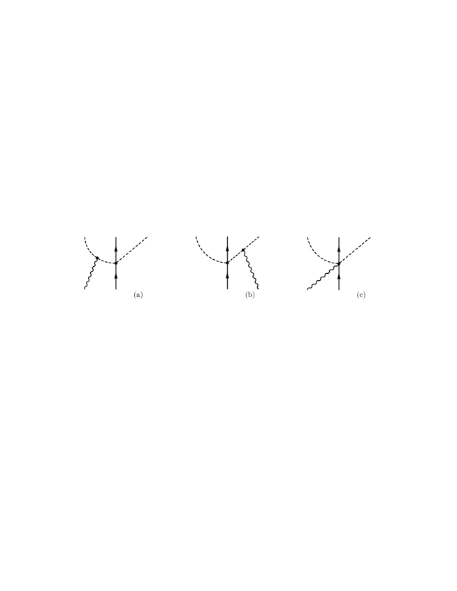
The contact term of Fig. 5 (c) is easily generated and assuming the reaction $\gamma M_{i}B_{i}\to M_{j}B_{j}$ the amplitude is given by

$$V_{ij}^{(\gamma)}=C_{ij}\;\frac{e}{4f_{i}f_{j}}\;(Q_{i}+Q_{j})\overline{u}(p^{\prime})\gamma^{\mu}u(p)\epsilon_{\mu}\;$$ (13)

with $Q_{i},Q_{j}$ the meson charges. In the Coulomb gauge this becomes

$$V_{ij}^{(\gamma)}=-C_{ij}\;\frac{e}{4f_{i}f_{j}}\;i\;\frac{\vec{\sigma}\times{\bf q}}{2M_{p}}\;{\vec{\epsilon}}\;(Q_{i}+Q_{j})$$ (14)

in the $\gamma p$ CM frame. Since the initial channel $i$ is $\pi^{0}p$, or channel number 1 in the order of the channels from Sec. II, we obtain

$$V_{1j}^{(\gamma)}=-C_{1j}\;\frac{e}{4f_{1}f_{j}}\;i\;\frac{\vec{\sigma}\times{\bf q}}{2M_{p}}\;{\vec{\epsilon}}\;\;Q_{j}.$$ (15)

It was shown in Ref. Nacher:1998mi that the meson pole terms of Fig. 5 (a), (b) are small compared to the amplitude of Eq. (15) for energies where the final particles are relatively close to threshold, as is the case here, both at the tree level or when the photon couples to the mesons within loops. The coupling of the photon to the baryon components was also small and will be neglected here, as was done in Ref. Nacher:1998mi .

Before we proceed to unitarize the amplitude, it is worth looking at the structure of Eq. (15) which contains the ordinary magnetic moment of the proton. It is logical to think that a realistic amplitude should contain also the anomalous part of the magnetic moment. This is indeed the case if one considers the effective Lagrangians given in Ref. stein

$${\cal L} = -\;\frac{i}{4M_{p}}\;b_{6}^{F}\left\langle\overline{B}\left[S^{\mu},S^{\nu}\right]\left[F^{+}_{\mu\nu},B\right]\right\rangle$$ (16)

$$-\;\frac{i}{4M_{p}}\;b_{6}^{D}\left\langle\overline{B}\left[S^{\mu},S^{\nu}\right]\{F^{+}_{\mu\nu},B\}\right\rangle$$

with

$$F_{\mu\nu}^{+} = -e\left(u^{\dagger}QF_{\mu\nu}\;u+uQF_{\mu\nu}\;u^{\dagger}\right),$$

$$F_{\mu\nu} = \partial_{\mu}A_{\nu}-\partial_{\nu}A_{\mu}$$ (17)

with $M_{p}$ the proton mass and $A_{\mu}$ the electromagnetic field. The operator $Q$ in Eq. (17) is the quark charge matrix $Q={\rm diag}(2,-1,-1)/3$ and $S^{\mu}$ is the spin matrix which in the rest frame becomes $(0,\vec{\sigma}/2)$. In Ref. Jido:2002yz the Lagrangians of Eq. (16) were used to determine the magnetic moment of the $\Lambda(1405)$. In the Coulomb gauge one has for an incoming photon

$$\left[S^{\mu},S^{\nu}\right]F_{\mu\nu}\to\left(\vec{\sigma}\times{\bf q}\right){\vec{\epsilon}}$$ (18)

and, thus, the vertex from the Lagrangian of Eq. (16) can be written as

$${\cal L}\to e\;\frac{\vec{\sigma}\times{\bf q}}{2M_{p}}\;{\vec{\epsilon}}\;\Big{(}\frac{i}{2}\;b_{6}^{F}\left\langle\overline{B}\left[\left(u^{\dagger}Qu+uQu^{\dagger}\right),B\right]\right\rangle$$

$$+\frac{i}{2}\;b_{6}^{D}\left\langle\overline{B}\{\left(u^{\dagger}Qu+uQu^{\dagger}\right),B\}\right\rangle\Big{)}.$$ (19)

Expanding the terms up to two meson fields leads to contact vertices with the same structure as Eq. (14). Taking $u=1$ in Eq. (19), and hence with no meson fields, provides the full magnetic moments of the octet of baryons from where one obtains the values of the coefficients stein ; Jido:2002yz

$$b_{6}^{D}=2.40,\quad b_{6}^{F}=1.82.$$

It is easy to see Jido:2002yz that by setting $b_{6}^{D}=0$, $b_{6}^{F}=1$, one obtains the ordinary magnetic moments of the baryons without the anomalous contribution. Similarly, taking the same values of $b_{6}^{D}$, $b_{6}^{F}$ one obtains Eq. (14) for the vertices $\gamma MMBB$. This is easily seen by explicitly evaluating the matrix elements of Eq. (19) which lead to the amplitude

$$-it_{ij}^{\gamma}=-\;\frac{e}{2M_{p}}(\vec{\sigma}\times{\bf q}){\vec{\epsilon}}\;\frac{1}{2f_{i}f_{j}}\left[X_{ij}b_{6}^{D}+Y_{ij}b_{6}^{F}\right]$$ (20)

where the coefficients $X_{ij}$ and $Y_{ij}$ are given in Table 3.

Table 3: $X_{1j}$ and $Y_{1j}$ coefficients for the anomalous magnetic moment.

	$\pi^{0}p$	$\pi^{+}n$	$\eta p$	$K^{+}\Sigma^{0}$	$K^{+}\Lambda$	$K^{0}\Sigma^{+}$
$X_{1j}$	$0$	$\sqrt{2}$	$0$	$\frac{1}{2}$	$-\frac{1}{2\sqrt{3}}$	$0$
$Y_{1j}$	$0$	$\sqrt{2}$	$0$	$-\frac{1}{2}$	$-\frac{\sqrt{3}}{2}$	$0$

The combination of the $Y_{1j}$ in Table 3 and the $C_{1j}$ of Table 1 shows the identity of Eq. (20) and Eq. (15) for the case of $b_{6}^{D}=0$, $b_{6}^{F}=1$.

III.1.1 Unitarization

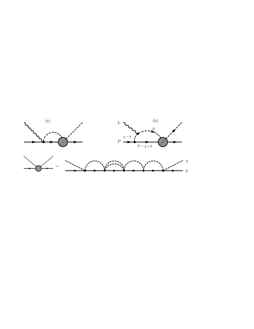
For the amplitude $\gamma p\to\pi^{0}\eta p$, the first thing to realize is that at tree level the amplitude is zero with the interactions from Eqs. (15) and (20). It is the unitarization and the coupled channel procedure that renders this amplitude finite and sizable. The unitarization procedure with the coupled channels allows the intermediate channels with charged mesons of Eq. (1) to be formed, even if some of them are not physically open. The scattering of these states leads finally to $\eta p$. Diagrammatically, this is depicted in Fig. 6

Figure 6: Unitarization of the transition amplitude for $\eta p$ production. The possible states (see table 1) for one and two loops are indicated.

which implicitly assumes the unitarization is implemented via the use of the Bethe-Salpeter equation (5) which generates the diagrams of Fig. 6.

Since $\eta p$ is channel 3 in our list of coupled channels, our final amplitude reads

$$T_{\gamma p\to\pi^{0}\eta p}=-i\sum_{j}\left(b_{6}^{D}X_{1j}+b_{6}^{F}Y_{1j}\right)\frac{e}{4f_{1}f_{j}}\;\frac{\vec{\sigma}\times{\bf q}}{2M_{p}}\;\vec{\epsilon}\;G_{j}(z)\;T^{(j3)}(z)\;,$$ (21)

where $G_{j}$ is the meson-baryon loop function which is obtained in Ref. Inoue:2001ip using dimensional regularization, and the $T^{(j3)}$ are the ordinary scattering matrices of the $\eta p$ and coupled channels from Eq. (5). The invariant kinematical argument $z$ is given by the invariant mass $M_{I}(\eta p)$ of the $\eta p$ system,

$$z=M_{I}$$ (22)

or, alternatively,

$$z=\left(s+m_{\pi}^{2}-2\sqrt{s}\;p_{\pi}^{0}\right)^{1/2}$$ (23)

with $p_{\pi}^{0}=({\bf p}_{\pi}^{2}+m_{\pi}^{2})^{1/2}$, when the amplitude is expressed in terms of the invariant mass $M_{I}(\pi^{0}p)$ of the $\pi^{0}p$ system.

One might also question why we do not unitarize the other $\pi^{0}$ with the $\eta$ or the proton. The reason has to do with the chosen kinematics. By being close to threshold the $\pi^{0}$ has a small momentum and is far from the region of the $a_{0}(980)$ resonance that could be created interacting with the $\eta$. The generation of the $\pi^{0}p$ invariant masses in the $\Delta(1232)$ region in the phase space that we investigate is more likely. However, as one can see from Fig. 5 an extra loop of the $\pi^{0}$ and $p$ lines produces a $\Delta(1232)$ which would involve an s-wave vertex and a p-wave vertex. This would vanish in the loop integration in the limit of large baryon masses. Later, we shall consider other diagrams in which the $\Delta(1232)$ is explicitly produced.

III.2 Kroll-Ruderman and meson pole term

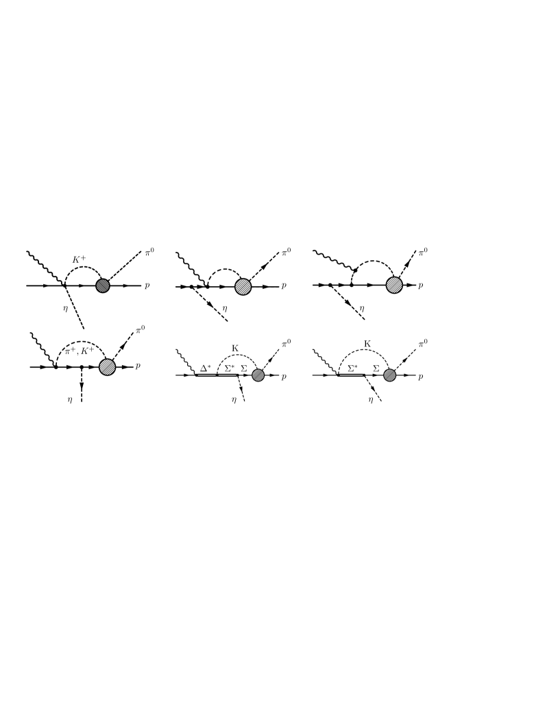
Next, we take into account diagrams which involve the $\gamma N\to\eta N$ amplitude which has been discussed in Sec. II.1, and which are shown in Fig. 7.

Figure 7: Kroll-Ruderman term and meson pole term as sub-processes in the $\pi^{0}\eta$ production.

With Eqs. (8) and (9) the amplitude for the diagrams in Fig. 7 is given by

$$(-iT_{\gamma p\to\pi^{0}\eta p})=\frac{D+F}{2f_{\pi}}\;\frac{M}{E_{N}({\bf k+p_{\pi}})}\;\frac{i}{E_{N}({\bf k})-p_{\pi}^{0}-E_{N}({\bf k+p_{\pi}})}\;(-iT_{\gamma p\to\eta p}(z))\;(-{\vec{\sigma}}\cdot{\bf p_{\pi}})$$ (24)

where $z$ takes the values given by Eq. (22) or (23).

III.2.1 Intermediate pion emission

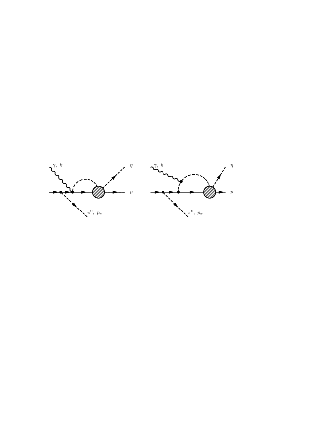
In addition to the diagrams considered above, there are additional diagrams in which the $\pi^{0}$ is produced inside the first meson-baryon loop as displayed in Fig. 8.

Figure 8: Pion emission from inside the first meson-baryon loop. Diagram (d) is required by gauge invariance.

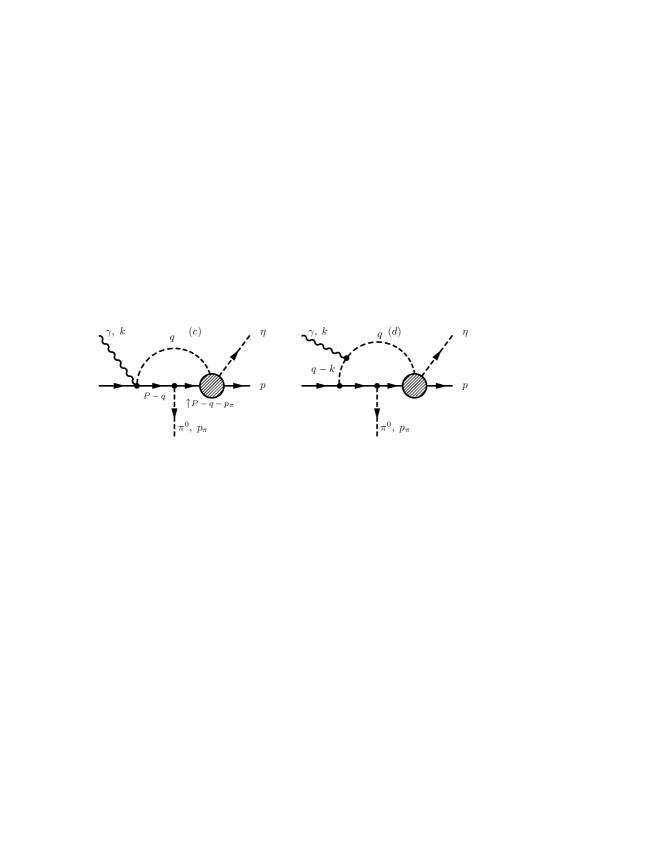
The amplitude for the channel $i$ for the sum of diagram (c) and (d) is given by

$$t^{i}_{(c)+(d)}(\sqrt{s}) = -\frac{e}{2f_{\pi}f_{i}}({\vec{\sigma}}\cdot{\bf p_{\pi}})({\vec{\sigma}}{\vec{\epsilon}})\>[a_{i}\>(D+F)+b_{i}\>(D-F)][a^{\prime}_{i}\>(D+F)+b^{\prime}_{i}\>(D-F)]$$ (25)

$$\times\;T^{(i3)}(z)\int\frac{d^{3}{\bf q}}{(2\pi)^{3}}\;\frac{1}{2\omega}\;\frac{M}{E_{M}(q)}\;\frac{1}{\sqrt{s}-\omega-E_{M}(q)+i\epsilon}\frac{M^{\prime}}{E_{M^{\prime}}({\bf q+p}_{\pi})}\;$$

$$\times\;\frac{1}{\sqrt{s}-\omega-p_{\pi}^{0}-E_{M^{\prime}}({\bf q+p}_{\pi})+i\epsilon}\left(1-\frac{{\vec{q}}_{\rm on}^{\;2}}{3\>q_{\rm on}^{0}\>k^{0}}\right)F_{\pi}(q-k)$$

where the index $i$ stands for our standard ordering of the channels in Eq. (1) and the only non-zero values of the $a_{i},a^{\prime}_{i},b_{i},b^{\prime}_{i}$ are: $a_{2}=-\frac{1}{\sqrt{2}},a^{\prime}_{2}=-1,a_{4}=b_{4}=\frac{1}{\sqrt{6}},a^{\prime}_{4}=\sqrt{\frac{2}{3}},b^{\prime}_{4}=-\frac{1}{\sqrt{6}},a_{5}=b_{5}=\frac{1}{\sqrt{6}},b^{\prime}_{5}=-\frac{1}{\sqrt{2}}$. Note that channel two has the external $\pi^{0}$ coupled to $n$, $n$ to the left and right in the diagram, channel four has the $\pi^{0}$ coupled to the $\Lambda$, $\Sigma$ to the left and right, and channel five has the $\pi^{0}$ coupled to the $\Sigma$, $\Lambda$ to the left and right. In the equation the variable $P-q$ refers to the baryon on the left (M) of the emitted $\pi^{0}$ and the variable $P-q-p_{\pi}$ to the right ($M^{\prime}$) of the emitted $\pi^{0}$ as shown in Fig. 8. The contribution of the terms in Fig. 8 is therefore given by the sum of Eq. (25) for the three non-vanishing channels.

In Eq. (25) we introduce the ordinary meson-baryon form factor $F_{\pi}$ of monopole type with $\Lambda$= 1.25 GeV as used in the two pion photoproduction Nacher:2000eq . It appears naturally in the meson pole term of Fig. 8 and, as done in Ref. Nacher:2000eq , it is also included in Fig. 8(c) (Kroll-Ruderman term) for reasons of gauge invariance. This form factor does not change much the results and it is approximated by taking the $q^{0}$ variable on shell and making an angle average of the $\vec{q}$ momentum. This is done to avoid fictitious poles in the $q^{0}$ integrations.

The meson pole term (d) in Fig. 8 is small and an approximation can be made for the intermediate pion at $q-k$ which is far off-shell. This concerns terms with mixed scalar products of the form ${\bf k\cdot q}$ that give only a small contribution when integrating over ${\bf q}$ in Eq. (25). Additionally, we have set in this term $q\equiv q_{\rm on}$, the on-shell momentum of the other meson at $q$. This is, considering the kinematics, a good approximation.

One can also have the pion emission from the final proton. However, this would imply having the $\pi N\to\eta N$ amplitude away from the $N^{*}(1535)$ resonance at a value $M_{I}=\sqrt{s}$ where the $\pi N\to\eta N$ amplitude would only provide a background term above the $N^{*}(1535)$ resonance. Once again the set of diagrams considered leads to small cross sections compared to the dominant terms to be considered later in the paper so further refinements are unnecessary.

III.3 Baryonic resonances in $\eta\pi^{0}$ production

In the present study, the $\eta\pi^{0}$ production is described as a two-step process: The first step consists in the photoproduction of two mesons and a baryon; the second step describes the subsequent transitions of meson-baryon $\to\eta p$ via the dynamically generated $N^{*}(1535)$ resonance. In particular, the first stage contains two pion photoproduction. For this part it is known that baryonic resonances such as $\Delta$’s and $N^{*}$’s can play an important role Nacher:2000eq ; GomezTejedor:1993bq ; GomezTejedor:1995pe ; Fix:2005if . For this reason we include the relevant mechanisms from Ref. Nacher:2000eq adapted to the present context. Fig. 9 shows the processes that are taken into account.

Figure 9: Terms with $\Delta^{*}(1700)$, $N^{*}(1520)$, and $\Delta(1232)$. The diagram on the right is the $\Delta$-Kroll-Ruderman term. The latter diagram implies also a meson pole contribution, required by gauge invariance, which is not separately plotted but is included in the calculation.

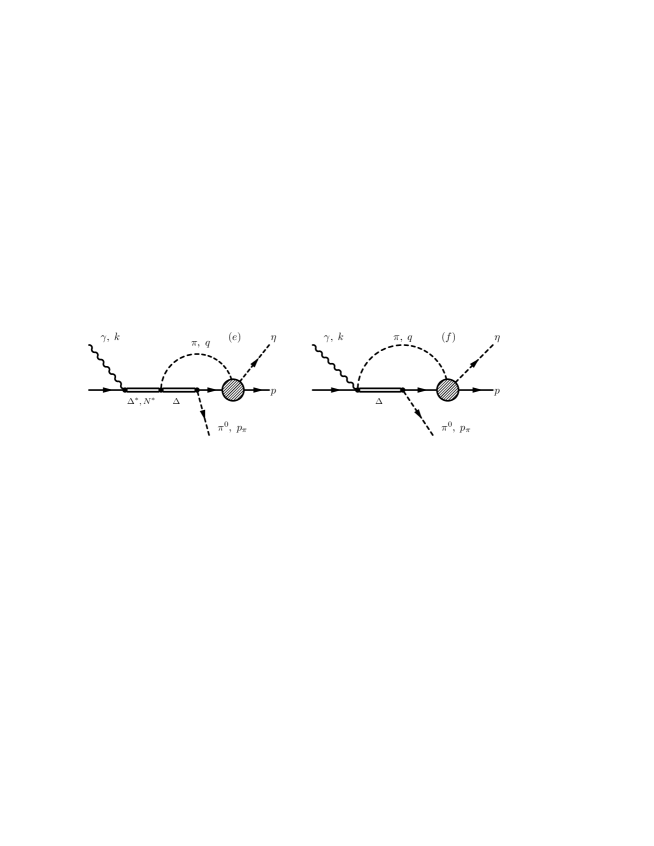
The $s$-wave character of the $N^{*}(1535)$ (gray blob in Fig. 9) discards all those processes from Ref. Nacher:2000eq where both pions couple in $p$-wave to the baryons, because the $\pi N$ loop function involving odd powers of $\vec{q}$ in the integral is zero in the heavy baryon limit. For the remaining processes, some contributions to the $\pi^{+}\pi^{0}$ and $\pi^{0}\pi^{0}$ cross sections are small as, e.g., from the Roper resonance. Finally, one is left with the $\Delta^{*}(1700)\Delta$, $N^{*}(1520)\Delta$, and $\Delta$-Kroll-Ruderman terms from Fig. 9. The latter implies also a pole term which is required by gauge invariance in the same way as in Fig. 8 (d). Since many resonances appear in this section we refer the reader to the notation used in the Introduction.

The amplitudes for diagrams (e) and (f) in Fig. 9 are given by

$$T_{\gamma p\to\pi^{0}\eta p}=\sum_{i=1,2}T^{(i,3)}(z)\frac{1}{(2\pi)^{2}}\int\limits_{0}^{\Lambda}dq\int\limits_{-1}^{1}dx\;t_{\Delta}^{i}\;\frac{q^{2}}{2\omega}\frac{M}{E}\frac{1}{\sqrt{s}-\omega-p_{\pi}^{0}-E+i\epsilon}\;\frac{1}{\sqrt{s_{\Delta}}-M_{\Delta}+i\;\frac{\Gamma(\sqrt{s_{\Delta}})}{2}}$$ (26)

with the sum only over the first two channels according to Eq. (1) and $\Lambda=1400$ MeV as in Sec. II.1. The meson energy $\omega$, baryon energy $E$ and energy of the $\Delta(1232)$ read

$$\omega^{2} = m^{2}+q^{2},$$

$$E^{2} = M^{2}+q^{2}+p_{\pi}^{2}+2qp_{\pi}x,$$

$$s_{\Delta} = \left(\sqrt{s}-\omega\right)^{2}-q^{2}$$ (27)

with meson mass $m$, baryon mass $M$, and $p_{\pi}=|{\bf p}_{\pi}|$ with $p_{\pi}^{0}=\sqrt{p_{\pi}^{2}+m_{\pi}^{2}}$. The argument $z$ is given by Eq. (22) or (23).

Using the notation from Ref. Nacher:2000eq the amplitudes $t_{\Delta}^{i}$, which can depend on the loop momentum, are given by:

$$t^{1}_{\Delta} = t_{\gamma p\to\pi^{+}\pi^{0}n}^{\Delta^{*}(1700)}+t_{\gamma p\to\pi^{+}\pi^{0}n}^{N^{*}(1520)}+t_{\gamma p\to\pi^{+}\pi^{0}n}^{\Delta-{\rm KR}}\;,$$ (28)

$$t^{2}_{\Delta} = t_{\gamma p\to\pi^{0}\pi^{0}n}^{\Delta^{*}(1700)}+t_{\gamma p\to\pi^{0}\pi^{0}n}^{N^{*}(1520)}+t_{\gamma p\to\pi^{0}\pi^{0}p}^{\Delta-{\rm KR}}$$ (29)

where

$$t_{\gamma p\to\pi^{+}\pi^{0}n}^{\Delta^{*}(1700)} = -i\;\frac{2}{\sqrt{3}}\;\frac{f^{*}_{\Delta N\pi}}{m_{\pi}}\;{\vec{S}}\cdot{\bf p}_{\pi}\left({\tilde{f}}_{\Delta^{*}\Delta\pi}+\frac{1}{3}\frac{{\tilde{g}}_{\Delta^{*}\Delta\pi}}{m_{\pi}^{2}}\;{\vec{q}}^{\;2}\right)G_{\Delta^{*}}(\sqrt{s}\>)$$ (30)

$$\left[g_{1}^{\prime}\;\frac{{\vec{S}}^{\dagger}\cdot{\bf k}}{2M}\;(\vec{\sigma}\times{\bf k})\vec{\epsilon}-i{\vec{S}}^{\dagger}\cdot{\vec{\epsilon}}\left(g_{1}^{\prime}(k^{0}+\frac{{\bf k}^{2}}{2M})+g_{2}^{\prime}\sqrt{s}\>k^{0}\right)\right],$$

$$t_{\gamma p\to\pi^{+}\pi^{0}n}^{N^{*}(1520)} = -i\;\frac{\sqrt{2}}{3}\;\frac{f^{*}_{\Delta N\pi}}{m_{\pi}}\;{\vec{S}}\cdot{\bf p}_{\pi}\left({\tilde{f}}_{N^{*^{\prime}}\Delta\pi}+\frac{1}{3}\frac{{\tilde{g}}_{N^{*^{\prime}}\Delta\pi}}{m_{\pi}^{2}}\;{\vec{q}}^{\;2}\right)G_{N^{*^{\prime}}}(\sqrt{s}\>)$$ (31)

$$\left[g_{1}\;\frac{{\vec{S}}^{\dagger}\cdot{\bf k}}{2M}\;(\vec{\sigma}\times{\bf k})\vec{\epsilon}-i{\vec{S}}^{\dagger}\cdot{\vec{\epsilon}}\left(g_{1}(k^{0}+\frac{{\bf k}^{2}}{2M})+g_{2}\sqrt{s}\>k^{0}\right)\right],$$

$$t_{\gamma p\to\pi^{+}\pi^{0}n}^{\Delta-{\rm KR}} = \frac{e\sqrt{2}}{9}\;\left(\frac{f^{*}_{\Delta N\pi}}{m_{\pi}}\right)^{2}\left(2{\bf p}_{\pi}-i({\vec{\sigma}}\times{\bf p_{\pi}})\right)\cdot{\vec{\epsilon}}\;F_{\pi}(q_{on}-k)\left(1-\frac{1}{3}\frac{{\vec{q}}_{\rm on}^{\;2}}{q_{\rm on}^{0}k^{0}}\right),$$ (32)

$$t_{\gamma p\to\pi^{0}\pi^{0}n}^{\Delta^{*}(1700)} = \frac{1}{2\sqrt{2}}\;t_{\gamma p\to\pi^{+}\pi^{0}n}^{\Delta^{*}(1700)},$$ (33)

$$t_{\gamma p\to\pi^{0}\pi^{0}n}^{N^{*}(1520)} = \sqrt{2}t_{\gamma p\to\pi^{+}\pi^{0}n}^{N^{*}(1520)},$$ (34)

$$t_{\gamma p\to\pi^{0}\pi^{0}p}^{\Delta-{\rm KR}} = 0.$$ (35)

We have already projected out the $s$-wave parts of the $\Delta^{*}(1700)\Delta\pi$ and $N^{*}(1520)\Delta\pi$ transitions that come from the term ${\tilde{g}}_{N^{*^{\prime}}\Delta\pi}/m_{\pi}^{2}\;{\vec{S}}^{\dagger}\cdot{\vec{p}}_{\pi}\;{\vec{S}}\cdot{\vec{p}}_{\pi}$, see Ref. Nacher:2000eq . The vector ${\bf p}_{\pi}$ depends implicitly on the invariant mass which will be specified later, Eqs. (46) or (48). The amplitudes in Eqs. (30)-(35) are formulated for real photons, which is the case we are considering here. The meson pole diagram related to the $\Delta$-Kroll-Ruderman term has been included in the last factor of Eq. (32) by making the same approximation as in Eq. (25) for the intermediate off-shell pion. The pion form factor $F_{\pi}$ (see Ref. Nacher:2000eq ) has to be inserted since the intermediate pion in the meson pole term is far off-shell. For the $\Delta^{*}$ propagator,

$$G_{\Delta^{*}}(\sqrt{s}\>)=\frac{1}{\sqrt{s}-M_{\Delta^{*}}+i\;\frac{\Gamma(\sqrt{s}\>)}{2}},$$ (36)

the (momentum-dependent) width according to its main decay channels has been taken into account: For $\Delta^{*}\to\pi N$ in $d$-wave, $\Delta^{*}\to N\rho(N\pi\pi)$, and $\Delta^{*}\to\Delta\pi(N\pi\pi)$ we obtain in a similar way as in Ref. Nacher:2000eq

$$\Gamma_{\Delta^{*}\to N\pi}(\sqrt{s}\>) = \Gamma_{\Delta^{*}\to N\pi}(M_{\Delta^{\star}})\;\frac{q_{\rm CM}(\sqrt{s}\>)^{5}}{q_{\rm CM}(M_{\Delta^{*}})^{5}},$$

$$\Gamma_{\Delta^{*}\to N\rho[\pi\pi]}(\sqrt{s}\>) = \frac{M_{N}}{6(2\pi)^{3}}\frac{m_{\Delta^{*}}}{\sqrt{s}}g_{\rho}^{2}f_{\rho}^{2}\int d\omega_{1}\;d\omega_{2}\;|D_{\rho}(q_{1}+q_{2})|^{2}({\bf q}_{1}-{\bf q}_{2})^{2}\Theta(1-|A|),$$

$$A = \frac{(\sqrt{s}-\omega_{1}-\omega_{2})^{2}-M_{N}^{2}-{\bf q}_{1}^{2}-{\bf q}_{2}^{2}}{2|{\bf q}_{1}||{\bf q}_{2}|},$$

$$\Gamma_{\Delta^{*}\to\Delta\pi[N\pi\pi]} = \frac{15}{16\pi^{2}}\int dM_{I}\;\frac{M_{I}\;k(M_{I})}{4\pi\sqrt{s}\>}\;\frac{\Gamma_{\Delta\to N\pi}(M_{I})\left(|A_{s}|^{2}+|A_{d}|^{2}\right)}{(M_{I}-M_{\Delta})^{2}+\left(\frac{\Gamma_{\Delta\to N\pi}(M_{I})}{2}\right)^{2}}\;\Theta(\sqrt{s}-M_{I}-m_{\pi})\;.$$

Here, $q_{\rm CM}(\sqrt{s}\>)$ is the CM momentum of the pion and the nucleon and $\Gamma_{\Delta^{*}\to N\pi}(M_{\Delta^{\star}})$ is determined through the branching ratio into that channel. For the decay into $N\rho$, $g_{\rho}=2.6$ is the $\Delta^{*}N\rho$ coupling, also determined through the branching ratio. Furthermore, $f_{\rho}=6.14$ is the $\rho\pi\pi$ coupling, $q_{i}=(\omega_{i},{\bf q}_{i})$, $i=1,2$ the four-momentum of the outgoing pions, and $D_{\rho}$ the $\rho$ propagator incorporating the $\rho$ width. For the decay into $\Delta\pi$, the finite width of the $\Delta$, $\Gamma_{\Delta\to N\pi}$, has been taken into account by performing the convolution. For the partial amplitudes $A_{s}$ and $A_{d}$ of the $\Delta^{*}$ decay into $\Delta\pi$ in $s$ and $d$-wave, see Ref. Nacher:2000eq . The $N^{*}(1520)$ propagator is dressed in a similar way with the analytic expressions given in Ref. Nacher:2000eq .

III.4 $SU(3)$ couplings of the $\Delta^{*}(1700)$ and background terms

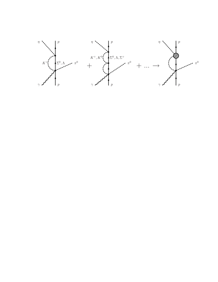
In Ref. Sarkar:2004jh the rescattering of the $0^{-}$ meson octet with the $3/2^{+}$ baryon decuplet leads to a set of dynamically generated resonances, one of which has been identified with the $\Delta^{*}(1700)$. The advantage of such a microscopic model is that couplings of the resonance to decay channels are predicted which have not yet been determined experimentally. In particular, the analytic continuation of the amplitude to the complex plane provides at the pole position the isospin $3/2$ couplings of the resonance to $\eta\Delta$ and $K\Sigma^{*}$. Identifying the pole with the $\Delta^{*}(1700)$ we can incorporate the model from Ref. Sarkar:2004jh in the present study in the diagrammatic way as indicated on the left side of Fig. 10, with the $\gamma p\Delta^{*}$ coupling from Ref. Nacher:2000eq .

Figure 10: Left side: Coupling of the dynamically generated $\Delta^{*}(1700)$ to $K\Sigma^{*}$ and $\eta\Delta$. The loop is given by $\eta\Delta^{+}p$, $K^{+}\Sigma^{*0}\Lambda$, or $K^{0}\Sigma^{*+}\Sigma^{+}$. Right side: $\Sigma^{*}$ Kroll-Ruderman term.

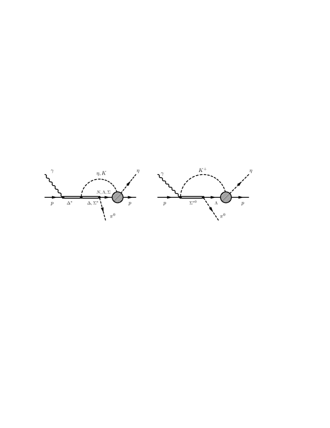
This procedure can be regarded as a first step towards the incorporation of dynamically generated $3/2^{-}$ resonances in the two meson photoproduction. In further studies, the initial $\gamma p\to\Delta^{*}$ process could be included in the microscopic model of Ref. Sarkar:2004jh in a similar way as was done here for the $\gamma pN^{*}(1535)$ coupling in Sec. II.1. However, phenomenologically, the procedure followed here is reliable.

The $\Delta^{*}(1700)\Delta\eta$ and $\Delta^{*}(1700)\Sigma^{*}K$ couplings from Ref. Sarkar:2004jh are given up to a global sign by $g_{\eta}=1.7-i1.4$ and $g_{K}=3.3+i0.7$, respectively. However, in Ref. Sarkar:2004jh the coupling to $\Delta\pi$ is also given, $g_{\Delta}=0.5+i\;0.8$. The sign of the real part and the order of magnitude agree with the empirical analysis of the $\Delta^{*}(1700)\to\pi\Delta$ decay that we are using thus far Nacher:2000eq ; hence, we take for $g_{\eta}$ and $g_{K}$ the values quoted above. We note that the cross section is almost independent of the global sign, whereas there are some minor differences in the invariant mass spectra.

Having included the $\Sigma^{*}$ in the $\Delta^{*}$ decay it is straightforward to consider also the corresponding $\Sigma^{*}$-Kroll-Ruderman term given on the right side of Fig. 10. This term, together with the other ones from this section, allows for an extension of the model to higher energies, where the intermediate $\Delta(1232)$ from the processes of Sec. III.3 is off-shell but the $\Sigma^{*}(1385)$ is on-shell.

For the baryon decuplet baryon octet meson octet vertices, and the corresponding Kroll-Ruderman vertex, we take the effective Lagrangian from Ref. Butler:1992pn ,

$${\cal L}={\cal C}\left(\overline{T}_{\mu}A^{\mu}B+{\overline{B}}A_{\mu}T^{\mu}\right)$$ (38)

with the same phase phase conventions for the states of the decuplet as taken there, which is the same one taken in Ref. Sarkar:2004jh . This allows us to relate all the couplings to the one of $\Delta\pi N$. Up to a different phase, these factors agree with those used in Ref. Oset:2000eg .

The corresponding amplitudes for the diagrams in Fig. 10 read now:

$$t_{\eta\Delta^{+}p}^{(3)} = -\sqrt{\frac{2}{3}}\;g_{\eta}\;\frac{\;f^{*}_{\Delta N\pi}}{m_{\pi}}\;G_{\Delta^{*}}(\sqrt{s})\;{\vec{S}}\cdot{\bf p}_{\pi}\left[-ig_{1}^{\prime}\;\frac{{\vec{S}}^{\dagger}\cdot{\bf k}}{2M}\;(\vec{\sigma}\times{\bf k})\vec{\epsilon}-{\vec{S}}^{\dagger}\cdot{\vec{\epsilon}}\left(g_{1}^{\prime}(k^{0}+\frac{{\bf k}^{2}}{2M})+g_{2}^{\prime}\sqrt{s}\;k^{0}\right)\right],$$ (39)

$$t_{K^{+}\Sigma^{*0}\Lambda}^{(5)} = 1.15\sqrt{\frac{24}{25}}\;g_{K}\;\frac{D+F}{2f_{\pi}}\;G_{\Delta^{*}}(\sqrt{s})\vec{S}\cdot{\bf p}_{\pi}\left[-ig_{1}^{\prime}\frac{\vec{S}^{\dagger}\cdot{\bf k}}{2M}(\vec{\sigma}\times{\bf k})\cdot\vec{\epsilon}-\vec{S}^{\dagger}\cdot\vec{\epsilon}\left(g_{1}^{\prime}(k^{0}+\frac{{\bf k}^{2}}{2M})+g_{2}^{\prime}\sqrt{s}\;k^{0}\right)\right],$$ (40)

$$t_{K^{0}\Sigma^{*+}\Sigma^{+}}^{(6)} = \frac{2}{5}\frac{D+F}{2f_{\pi}}\;g_{K}\;G_{\Delta^{*}}(\sqrt{s})\vec{S}\cdot{\bf p}_{\pi}\left[-ig_{1}^{\prime}\frac{\vec{S}^{\dagger}\cdot{\bf k}}{2M}(\vec{\sigma}\times{\bf k})\cdot\vec{\epsilon}-\vec{S}^{\dagger}\cdot\vec{\epsilon}\left(g_{1}^{\prime}(k^{0}+\frac{{\bf k}^{2}}{2M})+g_{2}^{\prime}\sqrt{s}\;k^{0}\right)\right],$$ (41)

$$t_{\Sigma^{*}{\rm-KR}}^{(5)} = -\;1.15\;e\;\frac{4\sqrt{3}}{25}\left(\frac{D+F}{2f_{\pi}}\right)^{2}\left(2{\bf p}_{\pi}-i(\vec{\sigma}\times{\bf p}_{\pi})\right)\cdot\vec{\epsilon}$$ (42)

with $g_{\eta}$ and $g_{K}$ given in Ref. Sarkar:2004jh . In order to obtain the full amplitudes, $T_{\gamma p\to\pi^{0}\eta p}$, these $t$’s have to be inserted as $t_{\Delta}^{i}$ Eq. (26) but the sum over index $i$ goes now from three to six. The lower index for the amplitudes in Eqs. (39) - (42) indicates the particles in the loop to be considered in the evaluation of Eq. (26). The upper index indicates the channel number $i$ and therefore which $T^{(i3)}$ has to be chosen in Eq. (26). For the amplitudes from Eq. (40), (41), and (42), the $\Delta(1232)$ propagator in Eq. (26) has to be replaced with the $\Sigma^{*}(1385)$ one. The latter is defined in the same way as the $\Delta(1232)$ propagator and we take a momentum-dependent width with $\Gamma_{\rm rest}=36$ MeV assuming the dominant $p$-wave decay of the $\Sigma^{*}$ into $p\Lambda$. The numerical factor of 1.15 appearing in Eqs. (40) and (42) is a phenomenological correction factor from the SU(3) $\Sigma^{*}\pi\Lambda$ coupling in order to provide the empirical $\Sigma^{*}\to\pi\Lambda$ partial decay width.

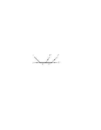
For the $\pi^{0}\eta p$ production, the $\Delta^{*}\Delta\eta$ coupling together with the subsequent $\Delta\to\pi^{0}p$ decay provides also a term at tree level as shown in Fig. 11.

Figure 11: Tree level process from the decay of the $\Delta^{*}(1700)$ to $\eta\Delta(1232)$.

The contribution for this reaction is simply given by

$$T_{\gamma p\to\pi^{0}\eta p}^{\rm BG} = t_{\eta\Delta^{+}p}^{(3)}\;G_{\Delta}(z^{\prime})$$ (43)

from Eq. (39). The invariant argument $z^{\prime}$ for this amplitude amplitude differs from $z$ of the former processes,

$$z^{\prime}=\left(s+m_{\eta}^{2}-2\sqrt{s}\;p_{\eta}^{0}\right)^{1/2},\quad z^{\prime}=M_{I}$$ (44)

with $p_{\eta}^{0}=({\bf p}_{\eta}^{2}+m_{\eta}^{2})^{1/2}$ depending on whether the amplitude is parametrized in terms of $M_{I}(\eta p)$ or $M_{I}(\pi^{0}p)$, respectively. We have explicitly tested that recoil corrections for the $\Delta(1232)$ decay ${\vec{S}}\cdot{\bf p}_{\pi}$ in Eq. (43), in the way they are applied in Ref. Nacher:2000eq , are negligible.

IV Results

In this section, invariant mass spectra $M_{I}(\eta p)$ and $M_{I}(\pi^{0}p)$ for the reaction $\gamma p\to\pi^{0}\eta p$ are predicted, together with the total cross section for this reaction. The corresponding observables for the $\pi^{0}K^{0}\Sigma^{+}$ final state are also given. These observables can be directly compared to ongoing experiments at the ELSA facilityMetag .

We evaluate the phase space integrals for the invariant mass distribution of $\eta p$ in the $\eta p$ CM system,

$$\frac{d\sigma}{dM_{I}(\eta p)}=\frac{1}{4(2\pi)^{5}}\frac{M_{p}M_{i}}{s-M_{p}^{2}}\;\frac{\tilde{p}_{\eta}p_{\pi}}{\sqrt{s}}\int\limits_{0}^{2\pi}d\phi_{\pi}\int\limits_{-1}^{1}d\cos\theta_{\pi}\int\limits_{0}^{2\pi}d\tilde{\phi}\int\limits_{-1}^{1}d\cos\tilde{\theta}\;\overline{\sum}\sum|T_{\gamma p\to\pi^{0}\eta p}|^{2}$$

(45)

with $\tilde{p}_{\eta}$ the modulus of the momentum ${\vec{\tilde{p}}}_{\eta}$ of the $\eta$ in the $\eta p$ rest frame ${\tilde{p}}_{\eta}=\lambda^{1/2}(M_{I}^{2},m_{\eta}^{2},M_{p}^{2})/(2M_{I})$ in terms of the ordinary Källen function where the direction of ${\vec{\tilde{p}}}_{\eta}$ is given by $\tilde{\phi}$ and $\tilde{\theta}$. This vector is connected to ${\vec{p}_{\eta}}$ in the $\gamma p$ rest frame by the boost

$${\vec{p}}_{\eta}=\left[\left(\frac{\sqrt{s}-\omega_{\pi}}{M_{I}}-1\right)\left(-\frac{{\vec{\tilde{p}}}_{\eta}{\vec{p}}_{\pi}}{{\vec{p}}_{\pi}^{\;2}}\right)+\frac{{\tilde{p}}_{\eta}^{0}}{M_{I}}\right]\left(-{\vec{p}}_{\pi}\right)+{\vec{\tilde{p}}}_{\eta}$$ (46)

where ${\tilde{p}}_{\eta}^{0}=\sqrt{{\vec{\tilde{p}}}_{\eta}^{\;2}+m_{\eta}^{2}}$ and the $\pi^{0}$ three momentum in the $\gamma p$ CM frame is given by the modulus $p_{\pi}=\lambda^{1/2}(s,M_{I}^{2},m_{\pi}^{2})/(2\sqrt{s})$ and the two angles $\phi_{\pi},\theta_{\pi}$. Furthermore, $\omega_{\pi}$ is the pion energy in the $\gamma p$ CM frame. In Eq. (45), $M_{p},M_{i}$ are proton mass and mass of the final baryon, in the present case also a proton ($i=3$ with the channel ordering from Eq. (1)). Eqs. (45) and (46) are a generalization of the corresponding expression in Ref. Nacher:1998mi as in the present case the amplitude depends explicitly on the angles of the particles.

The individual numerical contributions from the various processes from Sec. III are shown in Figs. 12, 13, and 14. We have chosen here a lab energy for the photon of $E_{\gamma}=$1.2 GeV so that the allowed invariant mass range is wide enough to distinguish the $N^{*}(1535)$ from pure phase space. On the other hand, this energy is low enough, so that unknown contributions from heavier resonances than the $\Delta^{*}(1700)$ should be small.

Figure 12: Invariant mass at $E_{\gamma}=1.2$ GeV. Dotted line: Contact interaction from Fig. 6 including the anomalous magnetic moment. Dashed dotted line: Meson pole plus Kroll-Ruderman term from Fig. 7. Double dashed dotted line: $\Delta^{*}(1700)K\Sigma^{*}$ transitions from Fig. 10, see Eqs. (40), (41). Solid line: Intermediate pion emission from Fig. 8.

Figure 13: Invariant mass at $E_{\gamma}=1.2$ GeV. Processes with explicit resonances. Dotted line: $\Delta^{*}(1700)\pi\Delta$ contribution from Fig. 9 (e), see Eqs. (30) and (33). Solid line: Contribution from $N^{*}(1520)\pi\Delta$ in Fig. 9 (e), see Eqs. (31) and (34). Dashed dotted line: $\Delta$-Kroll-Ruderman term from Fig. 9 (f), see Eq. (32). Double dashed dotted line: $\Sigma^{*}$-Kroll-Ruderman term from Fig. 10, see Eq. (42).

Figure 14: Invariant mass at $E_{\gamma}=1.2$ GeV. Dashed dotted line: $\Delta^{*}(1700)\eta\Delta$ transition and $\eta p\to\eta p$ rescattering from Fig. 10, see Eq. (39). Dotted line: Tree level process with $\Delta^{*}(1700)\eta\Delta$ transition but no rescattering, Fig. 11, see Eq. (43). Solid line: Coherent sum of all contributions, full model for the $N^{*}(1535)$. Dashed line: Coherent sum of all contributions, reduced model for $N^{*}(1535)$ from Sec. II (no vector particles in $t$-channel, no $\pi\pi N$ channel).

All contributions contain the resonant structure of the $N^{*}(1535)$ in the final state interaction, except the background term from Eq. (43). Although the shape of this contribution is similar to the resonant part, this is a combined effect of phase space and the intermediate $\Delta(1232)$ that becomes less off-shell at lower invariant masses for $E_{\gamma}=1.2$ GeV.

The individual contributions shown in Figs. 12, 13, and 14 are evaluated using the full model for the $N^{*}(1535)$ from Sec. II with the coherent sum indicated in Fig. 14, solid line. The coherent sum using the reduced model is displayed with the dashed line in Fig. 14. We take the difference between the two curves as an indication of the theoretical uncertainty as in the previous sections.

The first thing to note is that the peak position of the $N^{*}(1535)$ is lowered by some 20 MeV due to the interference of the dynamically generated resonance with the background term from Fig. 11. A width of 93 MeV for the $N^{*}(1535)$ has been extracted in Ref. Inoue:2001ip . In the invariant mass spectra the $N^{*}(1535)$ exhibits a considerably smaller width. This is for two reasons: First, the $N^{*}(1535)$ is situated close to the $\eta p$ threshold and the phase space cuts the lower energy tail. This is clearly visible in Fig. 15:

Figure 15: Modulus of the amplitude (full model for $N^{*}(1535)$) for the reaction $M_{i}B_{i}\to\eta p$ (left side) and $M_{i}B_{i}\to\pi^{0}p$ (right side). As these amplitudes appear squared in invariant mass spectra and total cross sections, they serve as a useful tool to distinguish dominant processes for the $\pi^{0}\eta p$ final state. Initial states: Dotted lines: $\pi^{0}p$, Dashed lines: $\pi^{+}n$, Solid lines: $\eta p$, Dashed dotted line: $K^{+}\Sigma^{0}$, Double dashed dotted lines: $K^{+}\Lambda$, Triple dashed dotted lines: $K^{0}\Sigma^{+}$.

As the phase space factors in Eq. (45) are smooth functions around the $N^{\star}(1535)$ resonance, the shape of the curves in Figs. 12, 13, and 14 reflects the $N^{\star}(1535)$ resonance seen through a $|T|^{2}$ matrix involving the coupled channels.

The second reason for the narrow $N^{\star}(1535)$ is that at higher invariant mass the amplitude for the resonance is suppressed by the initial photoproduction mechanism: A closer inspection of the dominant resonant contributions as, e.g., from Eq. (39) shows that the $\Delta(1232)$ propagator in Eq. (26) of the first loop becomes more and more off-shell at higher $\eta p$ invariant masses which leads to a suppression of the spectrum for this kinematics. This effect is in fact so pronounced that the shape of the invariant mass distribution hardly changes if the $MB\to\eta p$ theoretical transition amplitudes are replaced in the scattering diagrams by the phenomenological ones given by Eq. (10). This is clearly seen in Fig. 16.

Figure 16: Phenomenological potential for the $MB\to\eta p$ transition at $E_{\gamma}=1.2$ GeV. With solid and dashed line, full and reduced model for the $N^{*}(1535)$ as in Fig. 14. Dotted line: Phenomenological potential in the meson-baryon $\to\eta p$ final state interaction for the diagrams from Figs. 6, 7, 8, 9, and 10.

The transitions $|T^{(i3)}|$ and $|T^{(i1)}|$ in Fig. 15 explain the size of some of the contributions in Figs. 12, 13, and 14 as they appear squared in invariant mass spectra and cross section. E.g., the $\pi N\to\eta p$ transitions on the left side of Fig. 15 are small which explains why the $\Delta$-Kroll-Ruderman term and the $N^{*}(1525)\pi\Delta$, $\Delta^{*}(1700)\pi\Delta$ transitions from Eqs. (30)-(35) contribute little, opposite to what was found in the two-pion photoproduction Nacher:2000eq . In contrast, the diagrams using $SU(3)$ Lagrangians without explicit resonances from Figs. 6, 7, and 8 contain $K\Lambda$ and $K\Sigma$ channels in the first loop so that the contributions are larger. The by far largest contributions in the rescattering part (Fig. 14) comes from the $\Delta^{*}(1700)\to\eta\Delta$ decay with the subsequent unitarization of $\eta p$. Indeed, the $\eta p\to\eta p$ scattering amplitude is very large as Fig. 15 shows. Additionally, the loop for this reaction in Fig. 10 contains a $\eta$ instead of a $\pi$, and the particles in the loop can be simultaneously on-shell, whereas for the $\pi\Delta N$ loop at least one particle is always further off-shell.

The diagrams with $\Sigma^{*}(1385)$ in the first loop are relatively large (Fig. 12) due to the large $\Delta^{*}(1700)K\Sigma^{*}$ coupling and the large $K\Sigma\to\eta p$ and $K\Lambda\to\eta p$ transitions from Fig. 15. However, the $\Sigma^{*}(1385)$ is off-shell at $E_{\gamma}=1.2$ GeV and the contribution can not become as big as the loop from the $\Delta^{*}(1700)\to\Delta\eta$ decay. Therefore, diagrams with a $\Delta^{*}(1700)K\Sigma^{*}$ coupling become more important at higher energies. From Fig. 15, right side, we can also directly read off that additional diagrams like those displayed in Fig. 17

Figure 17: Selection of diagrams with $\pi^{0}p$ being the final state of the rescattering instead of $\eta p$. These diagrams are suppressed.

which use $T^{(i1)}$ instead of $T^{(i3)}$ are small compared to their counterparts from Sec. III.

IV.1 Extension to higher energies

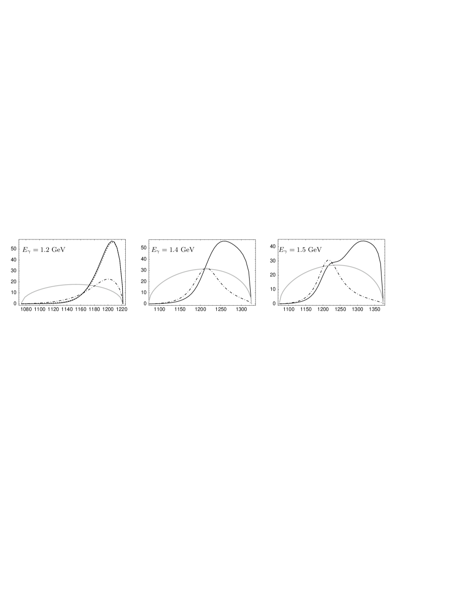
In Fig. 18

Figure 18: Invariant mass spectrum $\frac{d\sigma}{dM_{I}(\eta p)}\;[\mu{\rm b\;GeV}^{-1}]$ as a function of $M_{I}(\eta p)$ [MeV] for various photon lab energies $E_{\gamma}$. Solid and dashed lines: Full and reduced model for the $N^{*}(1535)$, respectively.

the results for the invariant mass distribution are shown for higher values of the incoming $\gamma$ momentum, $q_{\rm lab}=1.2-1.7$ GeV. The resonant shape of the $N^{*}(1535)$ is not modified if a bigger photon energy is chosen, only the size decreases slightly as the intermediate $\Delta^{*}(1700)$ of the dominant processes becomes off-shell. At higher incident photon energies, the peak of the $N^{*}(1535)$ moves back to its original position around 1520-1540 MeV (see, e.g., Fig. 1) as the interference of the dynamically generated $N^{*}(1535)$ with the tree level process from Fig. 11 becomes weaker.

A second maximum appears for $E_{\gamma}>\sim 1.5$ GeV and moves to higher invariant masses with increasing photon energy. This can be traced back to be a reflection of the $\Delta(1232)$ resonance in the tree level process from Fig. 11 which is on-shell around the position of the second peak. When predicting this double hump structure in the $\eta p$ invariant mass, one has to keep in mind that our model for the dynamically generated $N^{*}(1535)$ resonance underpredicts the width of this resonance (see, e.g., Figs. 1, 3). Furthermore, there are unknown contributions from resonances heavier than the $\Delta^{*}(1700)$ about which little is known and which can fill up the space in invariant mass between the two humps. As a result, we expect a separation of the two maxima not at $E_{\gamma}=1.5$ GeV as Fig. 18 suggests but at higher energies. Nevertheless, the tree level process from Fig. 11 contributes so strongly to the coherent sum that the double hump structure should be qualitatively visible in experiment.

In Fig. 19

Figure 19: Integrated cross section for the $\gamma p\to\pi^{0}\eta p$ reaction. Solid line: Full model for the $N^{*}(1535)$. Dashed line: Reduced model (see Sec. II). Dashed dotted line: Phenomenological potential for the $MB\to\eta p$ transition (only available up to $E_{\gamma}\sim 1.2$ GeV).

the integrated cross section is shown. There is a steep rise below $E_{\gamma}=1.2$ GeV simply due to growing phase space. Above that, the cross section grows slower and finally saturates. At high photon energies, the tree level process and the dynamically generated $N^{*}(1535)$ are almost completely separated in invariant mass (see Fig. 18) and we do not expect a further rise beyond 1.7 GeV within our approach, as the particles involved in the various processes become more and more off-shell. However, the narrow $N^{*}(1535)$ width of our model, together with unknown contributions from resonances heavier than the $\Delta^{*}(1700)$, lead to uncertainties at high photon energies which are hard to control.

As we have already seen in Fig. 16, the use of the wider phenomenological potential increases the cross section slightly (dashed dotted line), but it is remarkable how insensitive the cross section is to the actual width of the $N^{*}(1535)$, regarding the large difference in width between the results using the phenomenological potential or microscopic theory which we have seen for the $\gamma p\to\eta p$ reaction in Fig. 3.

IV.2 The $\pi^{0}p$ invariant mass

In the discussion of the last section we have seen that the $\Delta(1232)$ plays a prominent role in the $\pi^{0}\eta p$ photoproduction. For completeness, the invariant mass spectra for the $\pi^{0}p$ particle pair is given, which should show a signal of the $\Delta(1232)$. The phase space integrals are evaluated in the $\pi^{0}p$ rest frame and lead — similar to the expression in Eq. (45) — to the invariant mass distribution for $M_{I}(\pi^{0}p)$:

$$\frac{d\sigma}{dM_{I}(\pi^{0}p)}=\frac{1}{4(2\pi)^{5}}\frac{M_{p}M_{i}}{s-M_{p}^{2}}\;\frac{\tilde{p}_{\pi}p_{\eta}}{\sqrt{s}}\int\limits_{0}^{2\pi}d\phi_{\eta}\int\limits_{-1}^{1}d\cos\theta_{\eta}\int\limits_{0}^{2\pi}d\tilde{\phi}\int\limits_{-1}^{1}d\cos\tilde{\theta}\;\overline{\sum}\sum|T_{\gamma p\to\eta\pi^{0}p}|^{2}$$

(47)

with $M_{i}=M_{p}$ and with $\tilde{p}_{\pi}$ the modulus of the momentum ${\vec{\tilde{p}}}_{\pi}$ of the $\pi^{0}$ in the $\pi^{0}p$ rest frame ${\tilde{p}}_{\pi}=\lambda^{1/2}(M_{I}^{2},m_{\pi}^{2},M_{p}^{2})/(2M_{I})$ where the direction of ${\vec{\tilde{p}}}_{\pi}$ is given by $\tilde{\phi}$ and $\tilde{\theta}$. This vector is connected to ${\vec{p}_{\pi}}$ in the $\gamma p$ rest frame by the boost

$${\vec{p}}_{\pi}=\left[\left(\frac{\sqrt{s}-\omega_{\eta}}{M_{I}}-1\right)\left(-\frac{{\vec{\tilde{p}}}_{\pi}{\vec{p}}_{\eta}}{{\vec{p}}_{\eta}^{\;2}}\right)+\frac{{\tilde{p}}_{\pi}^{0}}{M_{I}}\right]\left(-{\vec{p}}_{\eta}\right)+{\vec{\tilde{p}}}_{\pi}$$ (48)

where ${\tilde{p}}_{\pi}^{0}=\sqrt{{\vec{\tilde{p}}}_{\pi}^{\;2}+m_{\pi}^{2}}$ and the $\eta$ three momentum in the $\gamma p$ CM frame is given by the modulus $p_{\eta}=\lambda^{1/2}(s,M_{I}^{2},m_{\eta}^{2})/(2\sqrt{s})$ and the two angles $\phi_{\eta},\theta_{\eta}$. Note that the invariant arguments for the solution of the Bethe-Salpeter equation (5) have changed compared to the case when the amplitude is expressed in terms of the $\eta p$ invariant mass, see Eqs. (22), (23), and (44).

The invariant mass distribution including all processes from this study is plotted in Fig. 20.

Figure 20: Invariant mass spectrum $\frac{d\sigma}{dM_{I}(\pi^{0}p)}\;[\mu{\rm b\;GeV}^{-1}]$ as a function of $M_{I}(\pi^{0}p)$ [MeV] for various photon lab energies $E_{\gamma}$. Solid lines: Full model for the $N^{*}(1535)$. Gray lines: Phase space only ($T$=const). Dashed dotted lines: Only tree level process from Fig. 11, see Eq. (43). Dotted line in plot for $E_{\gamma}=1.2$ GeV: Effect when including recoil corrections for the $\Delta\pi^{0}p$ vertex for the tree level diagram in Fig. 11.

We have checked explicitly for the individual processes and for the coherent sum of all processes that the integration over $M_{I}(\pi^{0}p)$ in Eq. (47) leads to the same values for the cross section as when integrating over the $\eta p$ invariant mass distribution from Eq. (45). In the plot for $E_{\gamma}=1.2$ GeV, the dotted line indicates the negligible effect of recoil corrections for the tree level process from Fig. 11 as described below Eq. (44).

In Fig. 20 we observe at $E_{\gamma}=1.2$ GeV a shift of strength towards higher invariant masses compared to the pure phase space (gray line) obtained by setting $T=$ const in Eq. (47). This is caused by the low energy tail of the $\Delta(1232)$ from the tree level process from Fig. 11, indicated with the dashed-dotted line. Indeed, at higher photon energies, the intermediate $\Delta(1232)$ in this process shows up as a shoulder at $E_{\gamma}=1.5$ GeV, and as a clear peak beyond. Additionally, there is a shift of strength towards higher invariant masses that results in a maximum which moves with energy, as it becomes apparent at $E_{\gamma}=1.5$ GeV. This is a reflection of the $N^{*}(1535)$ resonance that becomes on-shell around these invariant masses, in full analogy to the reflection of the $\Delta(1232)$ resonance in the $\eta p$ invariant mass spectra in Fig. 18. As we have already argued in Sec. IV.1, the separation of the two peaks might happen at higher values of the incident photon energy but should be qualitatively visible in experiment.

At this point we would like to make some comments concerning the accuracy of our results. If one looks at the results obtained for the $\gamma p\to\eta p$ cross section in Fig. 3 we can see that except in the low energy regime close to threshold, we have large discrepancies between the three options and also with experiment. The agreement can be considered just qualitatively. It is clear that some background and the contribution of the $N^{*}(1650)S_{11}$ might be missing and that in any case the theoretical uncertainties from different acceptable options are as big as 20-25 % at some energies. We should not expect better agreement with experiment in the $\gamma p\to\pi^{0}\eta p$ reaction which requires the $\gamma p\to\eta p$ amplitude in some terms (see Fig. 7). However, as we have discussed, these terms give a small contribution to the total amplitude, since the largest contribution comes from the tree level diagram of Fig. 11 and its unitarization in Fig. 10. Thus, at the end, the uncertainties in the result for the $\eta p$ invariant mass distribution, as seen in Fig. 16, are smaller than those of Fig. 3. Furthermore, when one integrates over the $\eta p$ invariant mass distribution, the uncertainties in the calculation in the total cross section are relatively small, although we would not claim a precision of better than 20 % considering all the different sources that enter the calculation. Given the complexity of the model, such an uncertainty is not easy to decrease at the present time, but it is more than acceptable for this first model of the reaction.

IV.3 The reaction $\gamma p\to\pi^{0}K^{0}\Sigma^{+}$

Figure 21: Tree level contribution for the $\pi^{0}K^{0}\Sigma^{+}$ final state.

The $\gamma p\to\pi^{0}K^{0}\Sigma^{+}$ reaction is calculated in a similar way as in the last sections for the $\pi^{0}\eta p$ final state as the coupled channel formalism for the $N^{*}(1535)$ contains the $K^{0}\Sigma^{+}$ final state in a natural way. There is, however, a different tree level diagram as displayed in Fig. 21 with the amplitude

$$T_{\gamma p\to\pi^{0}K^{0}\Sigma^{+}}^{\rm BG} = \frac{2}{5}\frac{D+F}{2f_{\pi}}\;g_{K}\;G_{\Sigma^{*}}(z^{\prime\prime})\;G_{\Delta^{*}}(\sqrt{s})\vec{S}\cdot{\bf p}_{\pi}\left[-ig_{1}^{\prime}\frac{\vec{S}^{\dagger}\cdot{\bf k}}{2M}(\vec{\sigma}\times{\bf k})\cdot\vec{\epsilon}-\vec{S}^{\dagger}\cdot\vec{\epsilon}\left(g_{1}^{\prime}(k^{0}+\frac{{\bf k}^{2}}{2M})+g_{2}^{\prime}\sqrt{s}\;k^{0}\right)\right]$$

where

$$z^{\prime\prime}=\left(s+m_{K^{0}}^{2}-2\sqrt{s}\;p_{K^{0}}^{0}\right)^{1/2}$$ (50)

in analogy to Eq. (44), when expressing the amplitude in terms of the $K^{0}\Sigma^{+}$ invariant mass. The $\Sigma^{*}(1385)$ propagator $G_{\Sigma^{*}}$ has been given its width as explained below Eq. (42). Note that $T^{BG}_{\gamma p\to\pi^{0}K^{0}\Sigma^{+}}=t^{(6)}_{K^{0}\Sigma^{*+}\Sigma^{+}}G_{\Sigma^{*}}(z^{\prime\prime})$ with $t^{(6)}_{K^{0}\Sigma^{*+}\Sigma^{+}}$ from Eq. (41) in analogy to Eq. (43). For the contributions with rescattering, we simply have to choose the $(i,6)$ channel instead of the $(i,3)$ channel in $T^{(ij)}$ from Eq. (5), in the ordering of the channels from Eq. (1). This means the replacement $T^{(j3)}\to T^{(j6)}$ in Eq. (21) and accordingly for the rest of the contributions. The invariant mass distribution is obtained from a similar formula as Eq. (45) with $M_{i}=M_{\Sigma^{+}}$ and is plotted in Fig. 22.

Figure 22: Invariant mass spectrum for the reaction $\gamma p\to\pi^{0}K^{0}\Sigma^{+}$ for two photon lab energies $E_{\gamma}$. Solid lines: full model for the $N^{*}(1535)$. Dashed lines: reduced model for the $N^{*}(1535)$. Dotted lines: Only tree level process from Fig. 21.

The tree level contribution from Fig. 21, dotted line, dominates the spectrum. The reaction is situated at much higher energies than the $\gamma p\to\pi^{0}\eta p$ process and the dynamically generated $N^{*}(1535)$ is off-shell for the entire invariant mass range. Thus, the rescattering part appears as a uniform background. The tree level process shows a pronounced maximum which moves with the incident photon energy. This situation is analogous to the moving peak of the $\Delta(1232)$ in Fig. 18 and reflects the $\Sigma^{*}(1385)$ which is on-shell around the peak position. The full and reduced model for the final state interaction (see Sec. II) differ considerably in Fig. 22 at $E_{\gamma}=1.7$ GeV (solid versus dashed line). This is due to the fact that the model for the $N^{*}(1535)$ becomes uncertain at these high energies as it differs from the $\pi N\to\pi N$ partial wave analysis from Ref. Arndt:2003if above $\sqrt{s}\sim 1600$ MeV. At lower energies, the differences are smaller. In any case, in the energy range studied here, the dominant term is provided by the tree level diagram of Fig. 21.

The integrated cross section is displayed in Fig. 23.

Figure 23: Integrated cross section for the $\gamma p\to\pi^{0}K^{0}\Sigma^{+}$ reaction. Solid line: Full model for the $N^{*}(1535)$. Dashed line: Reduced model for the $N^{*}(1535)$. Dotted line: Contribution from the tree level diagram in Fig. 21.

Comparing with Fig. 19 it becomes obvious that the production of $\pi^{0}K^{0}\Sigma^{+}$ is highly suppressed. This is a combined effect of the $\Delta^{*}(1700)$ and the $N^{*}(1535)$ being off shell which we quantify below. Both reactions are compared at an energy of 150 MeV above their respective thresholds, where both cross sections have become significantly different from zero. For the resulting photon energies of $E_{\gamma}=1202$ MeV and 1603 MeV for the $\pi^{0}\eta p$ and $\pi^{0}K^{0}\Sigma^{+}$ final states, respectively, we obtain $\sigma_{\pi^{0}\eta p}/\sigma_{\pi^{0}K^{0}\Sigma^{+}}=10.9$. First, this ratio is an effect of the positive interference between the dynamically generated $N^{*}(1535)$ with the large contribution of the tree level term from Fig. 11. Calculating the cross section by using this latter term only, $\sigma_{\pi^{0}\eta p}(1202\;{\rm MeV})$ decreases by a factor 2.0. Second, and more important, the $\Delta^{*}(1700)$ propagator from Eq. (36) is off shell for the higher photon energy, $|G_{\Delta^{*}}(1202\;{\rm MeV})|^{2}/|G_{\Delta^{*}}(1603\;{\rm MeV})|^{2}=5.4$. Multiplying these two factors, one obtains 10.8 which clarifies the origin of the factor 10.9 quoted above.

Turning the argument around, if the experiment sees a factor 10 suppression of the $\pi^{0}K^{0}\Sigma^{+}$ final state, compared to $\pi^{0}\eta p$, this can be easily explained by the dominant role of the $\Delta^{*}(1700)$ found in the present study.

Other resonances beyond the $\Delta^{*}(1700)$ can contribute at these high energies, and their omission produces uncertainties in the calculated cross section. However, assuming that we have included the relevant mechanisms in the present model, the suppression of the $\pi^{0}K^{0}\Sigma^{+}$ versus the $\pi^{0}\eta p$ final state is such a strong effect that it should be visible in experiment.

V Conclusions

In this paper we have studied the reactions $\gamma p\to\pi^{0}\eta p$ and $\gamma p\to\pi^{0}K^{0}\Sigma^{+}$ making use of a chiral unitary framework which considers the interaction of mesons and baryons in coupled channels and dynamically generates the $N^{*}(1535)$. This resonance appears from the $s$-wave rescattering of $\eta N$ and coupled channels. We have used general chiral Lagrangians for the photoproduction mechanisms and have shown that even if at tree level the amplitudes for these reactions are zero, the unitarization in coupled channels renders the cross sections finite by coupling the photon to intermediate charged meson channels that lead to the $\eta p$ and $K^{0}\Sigma^{+}$ in the final state through multiple scattering of the coupled channels.

The theoretical framework has been complemented by other ingredients, considering explicit excitation of resonances, whose couplings to photons are taken from experiment.

The interaction of the meson octet with the baryon decuplet leads to a set of dynamically generated resonances, one of which has been identified with the $\Delta^{*}(1700)$. The decay of this resonance into $\eta\Delta$ and $K\Sigma^{*}$, followed by the unitarization, or in other words, the $\Delta^{*}(1700)\to\pi^{0}N^{*}(1535)$ decay, provides in fact the dominant contribution to the $N^{*}(1535)$ peak in the invariant mass spectrum. A similar term provides also a tree level process which leads, together with the $N^{*}(1535)$, to a characteristic double hump structure in the $\eta p$ and $\pi^{0}p$ invariant mass at higher photon energies.

A virtue of this approach, concerning the $\eta p$ spectrum around the $N^{*}(1535)$, and a test of the nature of this resonance as a dynamically generated object, is that one can make predictions about cross sections for the production of the resonance without introducing the resonance explicitly into the formalism; only its components in the $(0^{-},1/2^{+})$ and $(0^{-},3/2^{+})$ meson-baryon base are what matters, together with the coupling of the photons to these components and their interaction in a coupled channel formalism. The reactions studied here also probe decay channels of the $\Delta^{*}(1700)\to\eta\Delta(1232),\Delta^{*}(1700)\to K\Sigma^{*}(1385)$ or transitions like $\eta p\to N^{*}(1535)\to\eta p$ which are predicted by the model and not measured yet.

We have made predictions for the cross sections and for invariant mass distributions in the case of the $\gamma p\to\pi^{0}\eta p$ reaction. For the second reaction under study, $\gamma p\to\pi^{0}K^{0}\Sigma^{+}$, we could see that in the regions not too far from threshold of the $\gamma p\to\pi^{0}K^{0}\Sigma^{+}$ reaction, the cross section for the latter one was much smaller than for the first reaction.

The measurement of both cross sections is being performed at the ELSA/Bonn Laboratory and hence the predictions are both interesting and opportune and can help us gain a better insight in the nature of some resonances, particularly the $N^{*}(1535)$ and the $\Delta^{*}(1700)$ in the present case.

References

- (1) N. Kaiser, P. B. Siegel and W. Weise, Phys. Lett. B 362 (1995) 23.
- (2) N. Kaiser, T. Waas and W. Weise, Nucl. Phys. A 612 (1997) 297
- (3) E. Oset and A. Ramos, Nucl. Phys. A 635 (1998) 99
- (4) J. C. Nacher, A. Parreno, E. Oset, A. Ramos, A. Hosaka and M. Oka, Nucl. Phys. A 678 (2000) 187
- (5) J. A. Oller and U. G. Meissner, Phys. Lett. B 500 (2001) 263
- (6) D. Jido, J. A. Oller, E. Oset, A. Ramos and U. G. Meissner, Nucl. Phys. A 725 (2003) 181
- (7) C. Garcia-Recio, M. F. M. Lutz and J. Nieves, Phys. Lett. B 582 (2004) 49
- (8) T. Inoue, E. Oset and M. J. Vicente Vacas, Phys. Rev. C 65 (2002) 035204
- (9) N. Isgur and G. Karl, Phys. Rev. D 18 (1978) 4187.
- (10) S. Capstick and W. Roberts, Phys. Rev. D 49 (1994) 4570
- (11) T. W. Chiu and T. H. Hsieh, Nucl. Phys. A 755, 471 (2005)
- (12) N. Nakajima, H. Matsufuru, Y. Nemoto and H. Suganuma, arXiv:hep-lat/0204014.
- (13) J. A. Oller, E. Oset and A. Ramos, Prog. Part. Nucl. Phys. 45 (2000) 157.
- (14) J. K. Ahn [LEPS Collaboration], Nucl. Phys. A 721 (2003) 715.
- (15) J. C. Nacher, E. Oset, H. Toki and A. Ramos, Phys. Lett. B 455 (1999) 55
- (16) V. Metag and M. Nanova, private communication.
- (17) J. C. Nacher, E. Oset, M. J. Vicente and L. Roca, Nucl. Phys. A 695, 295 (2001)
- (18) J. A. Gomez Tejedor and E. Oset, Nucl. Phys. A 571, 667 (1994).
- (19) J. A. Gomez Tejedor and E. Oset, Nucl. Phys. A 600, 413 (1996)
- (20) E. E. Kolomeitsev and M. F. M. Lutz, Phys. Lett. B 585, 243 (2004)
- (21) S. Sarkar, E. Oset and M. J. Vicente Vacas, Nucl. Phys. A 750, 294 (2005)
- (22) U. G. Meissner, Rep. Prog. Phys. 56 (1993) 903; V. Bernard, N. Kaiser and U. G. Meissner, Int. J. Mod. Phys. E4 (1995) 193.
- (23) G. Ecker, Prog. Part. Nucl. Phys. 35 (1995) 1.
- (24) J. Gasser and H. Leutwyler, Nucl. Phys. B250 (1985) 465, 517, 539.
- (25) M. Doring, E. Oset and M. J. Vicente Vacas, Phys. Rev. C 70, 045203 (2004)
- (26) R. A. Arndt, W. J. Briscoe, I. I. Strakovsky, R. L. Workman and M. M. Pavan, Phys. Rev. C 69, 035213 (2004)
- (27) A. M. Gasparyan, J. Haidenbauer, C. Hanhart and J. Speth, Phys. Rev. C 68, 045207 (2003)
- (28) J. Nieves and E. Ruiz Arriola, Phys. Rev. D 64, 116008 (2001)
- (29) Current (06/2005) fit of the SAID solution of photoproduction, http://gwdac.phys.gwu.edu/
- (30) J. A. Oller, E. Oset and J. R. Pelaez, Phys. Rev. D 59 (1999) 074001 [Erratum-ibid. D 60 (1999) 099906]
- (31) T. S. H. Lee, J. A. Oller, E. Oset and A. Ramos, Nucl. Phys. A 643 (1998) 402
- (32) F. Gross and D. O. Riska, Phys. Rev. C 36, 1928 (1987).
- (33) A. N. Kvinikhidze and B. Blankleider, Phys. Rev. C 60, 044003 (1999)
- (34) C. H. M. van Antwerpen and I. R. Afnan, Phys. Rev. C 52, 554 (1995)
- (35) H. Haberzettl, Phys. Rev. C 56, 2041 (1997)
- (36) B. Borasoy, P. C. Bruns, U. G. Meissner and R. Nissler, Phys. Rev. C 72, 065201 (2005)
- (37) U. G. Meissner and S. Steininger, Nucl. Phys. B 499 (1997) 349
- (38) D. Jido, A. Hosaka, J. C. Nacher, E. Oset and A. Ramos, Phys. Rev. C 66 (2002) 025203
- (39) A. Fix and H. Arenhovel, Eur. Phys. J. A 25, 115 (2005)
- (40) M. N. Butler, M. J. Savage and R. P. Springer, Nucl. Phys. B 399, 69 (1993)
- (41) E. Oset and A. Ramos, Nucl. Phys. A 679, 616 (2001)